Maximum mutual information (MMI) has become one of the two de facto methods for sequence-level training of speech recognition acoustic models. This paper aims to isolate, identify and bring forward the implicit modelling decisions induced by the design implementation of standard finite state transducer (FST) lattice based MMI training framework. The paper particularly investigates the necessity to maintain a preselected numerator alignment and raises the importance of determinizing FST denominator lattices on the fly. The efficacy of employing on the fly FST lattice determinization is…Apple Machine Learning Research
Non-Autoregressive Neural Machine Translation: A Call for Clarity
Non-autoregressive approaches aim to improve the inference speed of translation models by only requiring a single forward pass to generate the output sequence instead of iteratively producing each predicted token. Consequently, their translation quality still tends to be inferior to their autoregressive counterparts due to several issues involving output token interdependence. In this work, we take a step back and revisit several techniques that have been proposed for improving non-autoregressive translation models and compare their combined translation quality and speed implications under…Apple Machine Learning Research
Detect patterns in text data with Amazon SageMaker Data Wrangler
In this post, we introduce a new analysis in the Data Quality and Insights Report of Amazon SageMaker Data Wrangler. This analysis assists you in validating textual features for correctness and uncovering invalid rows for repair or omission.
Data Wrangler reduces the time it takes to aggregate and prepare data for machine learning (ML) from weeks to minutes. You can simplify the process of data preparation and feature engineering, and complete each step of the data preparation workflow, including data selection, cleansing, exploration, and visualization, from a single visual interface.
Solution overview
Data preprocessing often involves cleaning textual data such as email addresses, phone numbers, and product names. This data can have underlying integrity constraints that may be described by regular expressions. For example, to be considered valid, a local phone number may need to follow a pattern like [1-9][0-9]{2}-[0-9]{4}, which would match a non-zero digit, followed by two more digits, followed by a dash, followed by four more digits.
Common scenarios resulting in invalid data may include inconsistent human entry, for example phone numbers in various formats (5551234 vs. 555 1234 vs. 555-1234) or unexpected data, such as 0, 911, or 411. For a customer call center, it’s important to omit numbers such as 0, 911, or 411, and validate (and potentially correct) entries such as 5551234 or 555 1234.
Unfortunately, although textual constraints exist, they may not be provided with the data. Therefore, a data scientist preparing a dataset must manually uncover the constraints by looking at the data. This can be tedious, error prone, and time consuming.
Pattern learning automatically analyzes your data and surfaces textual constraints that may apply to your dataset. For the example with phone numbers, pattern learning can analyze the data and identify that the vast majority of phone numbers follow the textual constraint [1-9][0-9]{2}-[0-9][4]. It can also alert you that there are examples of invalid data so that you can exclude or correct them.
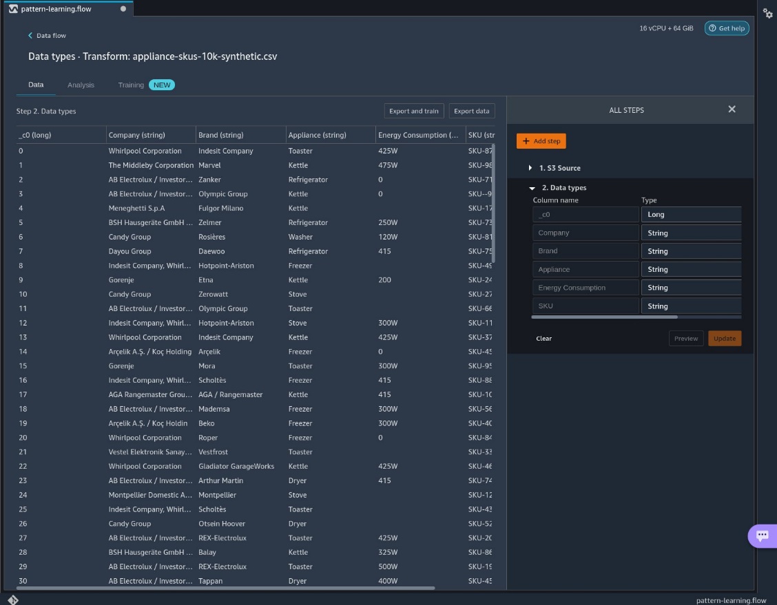
In the following sections, we demonstrate how to use pattern learning in Data Wrangler using a fictional dataset of product categories and SKU (stock keeping unit) codes.
This dataset contains features that describe products by company, brand, and energy consumption. Notably, it includes a feature SKU that is ill-formatted. All the data in this dataset is fictional and created randomly using random brand names and appliance names.
Prerequisites
Before you get started using Data Wrangler, download the sample dataset and upload it to a location in Amazon Simple Storage Service (Amazon S3). For instructions, refer to Uploading objects.
Import your dataset
To import your dataset, complete the following steps:
- In Data Wrangler, choose Import & Explore Data for ML.

- Choose Import.

- For Import data, choose Amazon S3.

- Locate the file in Amazon S3 and choose Import.
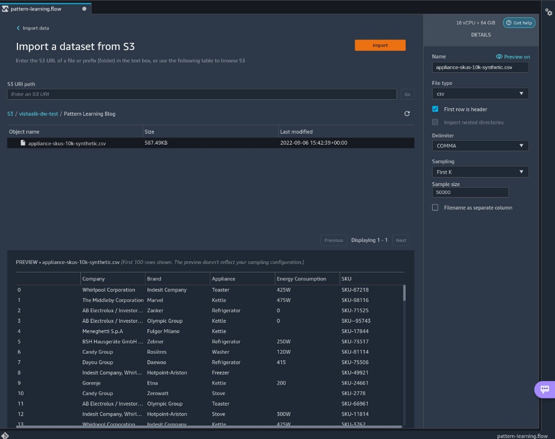
After importing, we can navigate to the data flow.
Get data insights
In this step, we create a data insights report that includes information about data quality. For more information, refer to Get Insights On Data and Data Quality. Complete the following steps:
- On the Data Flow tab, choose the plus sign next to Data types.
- Choose Get data insights.

- For Analysis type, choose Data Quality and Insights Report.
- For this post, leave Target column and Problem type blank.If you plan to use your dataset for a regression or classification task with a target feature, you can select those options and the report will include analysis on how your input features relate to your target. For example, it can produce reports on target leakage. For more information, refer to Target column.
- Choose Create.

We now have a Data Quality and Data Insights Report. If we scroll down to the SKU section, we can see an example of pattern learning describing the SKU. This feature appears to have some invalid data, and actionable remediation is required.

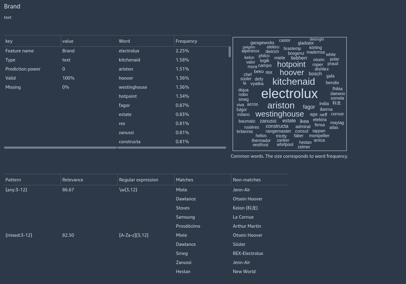
Before we clean the SKU feature, let’s scroll up to the Brand section to see some more insights. Here we see two patterns have been uncovered, indicating that that majority of brand names are single words consisting of word characters or alphabetic characters. A word character is either an underscore or a character that may appear in a word in any language. For example, the strings Hello_world and écoute both consist of word characters: H and é.
For this post, we don’t clean this feature.
View pattern learning insights
Let’s return to cleaning SKUs and zoom in on the pattern and the warning message.
As shown in the following screenshot, pattern learning surfaces a high-accuracy pattern matching 97.78% of the data. It also displays some examples matching the pattern as well as examples that don’t match the pattern. In the non-matches, we see some invalid SKUs.
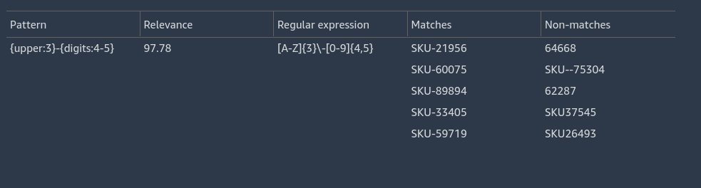
In addition to the surfaced patterns, a warning may appear indicating a potential action to clean up data if there is a high accuracy pattern as well as some data that doesn’t conform to the pattern.

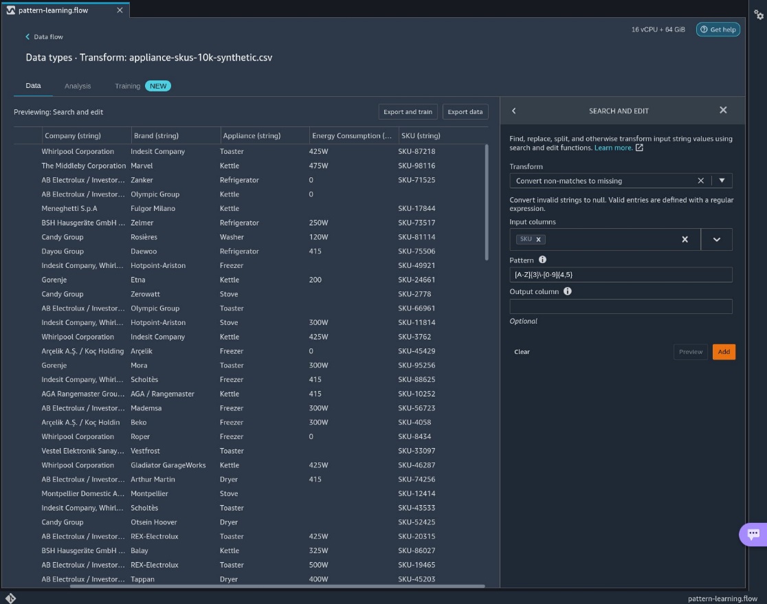
We can omit the invalid data. If we choose (right-click) on the regular expression, we can copy the expression [A-Z]{3}-[0-9]{4,5}.
Remove invalid data
Let’s create a transform to omit non-conforming data that doesn’t match this pattern.
- On the Data Flow tab, choose the plus sign next to Data types.
- Choose Add transform.

- Choose Add step.
- Search for
regexand choose Search and edit.

- For Transform, choose Convert non-matches to missing.
- For Input columns, choose
SKU. - For Pattern, enter our regular expression.
- Choose Preview, then choose Add.
Now the extraneous data has been removed from the features. - To remove the rows, add the step Handle missing and choose the transform Drop missing.
- Choose
SKUas the input column.
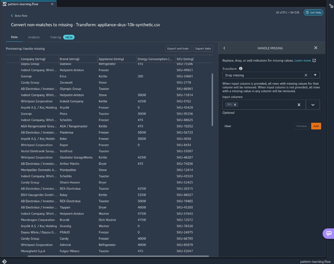
We return to our data flow with the erroneous data removed.

Conclusion
In this post, we showed you how to use the pattern learning feature in data insights to find invalid textual data in your dataset, as well as how to correct or omit that data.
Now that you’ve cleaned up a textual column, you can visualize your dataset using an analysis or you can apply built-in transformations to further process your data. When you’re satisfied with your data, you can train a model with Amazon SageMaker Autopilot, or export your data to a data source such as Amazon S3.
We would like to thank Nikita Ivkin for his thoughtful review.
About the authors
 Vishaal Kapoor is a Senior Applied Scientist with AWS AI. He is passionate about helping customers understand their data in Data Wrangler. In his spare time, he mountain bikes, snowboards, and spends time with his family.
 Zohar Karnin is a Principal Scientist in Amazon AI. His research interests are in the areas of large scale and online machine learning algorithms. He develops infinitely scalable machine learning algorithms for Amazon SageMaker.
 Ajai Sharma is a Principal Product Manager for Amazon SageMaker where he focuses on Data Wrangler, a visual data preparation tool for data scientists. Prior to AWS, Ajai was a Data Science Expert at McKinsey and Company, where he led ML-focused engagements for leading finance and insurance firms worldwide. Ajai is passionate about data science and loves to explore the latest algorithms and machine learning techniques.
 Derek Baron is a software development manager for Amazon SageMaker Data Wrangler
Reduce deep learning training time and cost with MosaicML Composer on AWS
In the past decade, we have seen Deep learning (DL) science adopted at a tremendous pace by AWS customers. The plentiful and jointly trained parameters of DL models have a large representational capacity that brought improvements in numerous customer use cases, including image and speech analysis, natural language processing (NLP), time series processing, and more. In this post, we highlight challenges commonly reported specifically in DL training, and how the open-source library MosaicML Composer helps solve them.
The challenge with DL training
DL models are trained iteratively, in a nested for loop. A loop iterates through the training dataset chunk by chunk and, if necessary, this loop is repeated several times over the whole dataset. ML practitioners working on DL training face several challenges:
- Training duration grows with data size. With permanently-growing datasets, training times and costs grow too, and the rhythm of scientific discovery slows down.
- DL scripts often require boilerplate code, notably the aforementioned double for loop structure that splits the dataset into minibatches and the training into epochs.
- The paradox of choice: several training optimization papers and libraries are published, yet it’s unclear which one to test first, and how to combine their effects.
In the past few years, several open-source libraries such as Keras, PyTorch Lightning, Hugging Face Transformers, and Ray Train have been attempting to make DL training more accessible, notably by reducing code verbosity, thereby simplifying how neural networks are programmed. Most of those libraries have focused on developer experience and code compactness.
In this post, we present a new open-source library that takes a different stand on DL training: MosaicML Composer is a speed-centric library whose primary objective is to make neural network training scripts faster via algorithmic innovation. In the cloud DL world, it’s wise to focus on speed, because compute infrastructure is often paid per use—even down to the second on Amazon SageMaker Training—and improvements in speed can translate into money savings.
Historically, speeding up DL training has mostly been done by increasing the number of machines computing model iterations in parallel, a technique called data parallelism. Although data parallelism sometimes accelerates training (not guaranteed because it disturbs convergence, as highlighted in Goyal et al.), it doesn’t reduce overall job cost. In practice, it tends to increase it, due to inter-machine communication overhead and higher machine unit cost, because distributed DL machines are equipped with high-end networking and in-server GPU interconnect.
Although MosaicML Composer supports data parallelism, its core philosophy is different from the data parallelism movement. Its goal is to accelerate training without requiring more machines, by innovating at the science implementation level. Therefore, it aims to achieve time savings which would result in cost savings due to AWS’ pay-per-use fee structure.
Introducing the open-source library MosaicML Composer
MosaicML Composer is an open-source DL training library purpose-built to make it simple to bring the latest algorithms and compose them into novel recipes that speed up model training and help improve model quality. At the time of this writing, it supports PyTorch and includes 25 techniques—called methods in the MosaicML world—along with standard models, datasets, and benchmarks
Composer is available via pip:
pip install mosaicmlSpeedup techniques implemented in Composer can be accessed with its functional API. For example, the following snippet applies the BlurPool technique to a TorchVision ResNet:
import logging

from composer import functional as CF
import torchvision.models as models
logging.basicConfig(level=logging.INFO)

model = models.resnet50()
CF.apply_blurpool(model)
Optionally, you can also use a Trainer to compose your own combination of techniques:
from composer import Trainer
from composer.algorithms import LabelSmoothing, CutMix, ChannelsLast

trainer = Trainer(
    model=.. # must be a composer.ComposerModel
    train_dataloader=...,
    max_duration="2ep",  # can be a time, a number of epochs or batches
    algorithms=[
        LabelSmoothing(smoothing=0.1),
        CutMix(alpha=1.0),
        ChannelsLast(),
    ]
)

trainer.fit()
Examples of methods implemented in Composer
Some of the methods available in Composer are specific to computer vision, for example image augmentation techniques ColOut, Cutout, or Progressive Image Resizing. Others are specific to sequence modeling, such as Sequence Length Warmup or ALiBi. Interestingly, several are agnostic of the use case and can be applied to a variety of PyTorch neural networks beyond computer vision and NLP. Those generic neural network training acceleration methods include Label Smoothing, Selective Backprop, Stochastic Weight Averaging, Layer Freezing, and Sharpness Aware Minimization (SAM).
Let’s dive deep into a few of them that were found particularly effective by the MosaicML team:
- Sharpness Aware Minimization (SAM) is an optimizer than minimizes both the model loss function and its sharpness by computing a gradient twice for each optimization step. To limit the extra compute to penalize the throughput, SAM can be run periodically.
- Attention with Linear Biases (ALiBi), inspired by Press et al., is specific to Transformers models. It removes the need for positional embeddings, replacing them with a non-learned bias to attention weights.
- Selective Backprop, inspired by Jiang et al., allows you to run back-propagation (the algorithms that improve model weights by following its error slope) only on records with high loss function. This method helps you avoid unnecessary compute and helps improve throughput.
Having those techniques available in a single compact training framework is a significant value added for ML practitioners. What is also valuable is the actionable field feedback the MosaicML team produces for each technique, tested and rated. However, given such a rich toolbox, you may wonder: what method shall I use? Is it safe to combine the use of multiple methods? Enter MosaicML Explorer.
MosaicML Explorer
To quantify the value and compatibility of DL training methods, the MosaicML team maintains Explorer, a first-of-its kind live dashboard picturing dozens of DL training experiments over five datasets and seven models. The dashboard pictures the pareto optimal frontier in the cost/time/quality trade-off, and allows you to browse and find top-scoring combinations of methods—called recipes in the MosaicML world—for a given model and dataset. For example, the following graphs show that for a 125M parameter GPT2 training, the cheapest training maintaining a perplexity of 24.11 is obtained by combining AliBi, Sequence Length Warmup, and Scale Schedule, reaching a cost of about $145.83 in the AWS Cloud! However, please note that this cost calculation and the ones that follow in this post are based on an EC2 on-demand compute only, other cost considerations may be applicable, depending on your environment and business needs.

Screenshot of MosaicML Explorer for GPT-2 training
Notable achievements with Composer on AWS
By running the Composer library on AWS, the MosaicML team achieved a number of impressive results. Note that costs estimates reported by MosaicML team consist of on-demand compute charge only.
- ResNet-50 training on ImageNet to 76.6% top-one accuracy for ~$15 in 27 minutes (MosaicML Explorer link)
- GPT-2 125M parameter training to a perplexity of 24.11 for ~$145 (MosaicML Explorer link)
- BERT-Base training to Average Dev-Set Accuracy of 83.13% for ~$211 (MosaicML Explorer link)
Conclusion
You can get started with Composer on any compatible platform, from your laptop to large GPU-equipped cloud servers. The library features intuitive Welcome Tour and Getting Started documentation pages. Using Composer in AWS allows you to cumulate Composer cost-optimization science with AWS cost-optimization services and programs, including Spot compute (Amazon EC2, Amazon SageMaker), Savings Plan, SageMaker automatic model tuning, and more. The MosaicML team maintains a tutorial of Composer on AWS. It provides a step-by-step demonstration of how you can reproduce MLPerf results and train ResNet-50 on AWS to the standard 76.6% top-1 accuracy in just 27 minutes.
If you’re struggling with neural networks that are training too slow, or if you’re looking to keep your DL training costs under control, give MosaicML on AWS a try and let us know what you build!
About the authors
 Bandish Shah is an Engineering Manager at MosaicML, working to bridge efficient deep learning with large scale distributed systems and performance computing. Bandish has over a decade of experience building systems for machine learning and enterprise applications. He enjoys spending time with friends and family, cooking and watching Star Trek on repeat for inspiration.
 Olivier Cruchant is a Machine Learning Specialist Solutions Architect at AWS, based in France. Olivier helps AWS customers – from small startups to large enterprises – develop and deploy production-grade machine learning applications. In his spare time, he enjoys reading research papers and exploring the wilderness with friends and family.
Integrating Arm Virtual Hardware with the TensorFlow Lite Micro Continuous Integration Infrastructure
A guest post by Matthias Hertel and Annie Tallund of Arm
Microcontrollers power the world around us. They come with low memory resources and high requirements for energy efficiency. At the same time, they are expected to perform advanced machine learning interference in real time. In the embedded space, countless engineers are working to solve this challenge. The powerful Arm Cortex-M-based microcontrollers are a dedicated platform, optimized to run energy-efficient ML. Arm and the TensorFlow Lite Micro (TFLM) team have a long-running collaboration to enable optimized inference of ML models on a variety of Arm microcontrollers.
Additionally, with well-established technologies like CMSIS-Pack, the TFLM library is ready to run on to 10000+ different Cortex-M microcontroller devices with almost no integration effort. Combining these two offers a great variety of platforms and configurations. In this article, we will describe how we have collaborated with the TFLM team to use Arm Virtual Hardware (AVH) as part of the TFLM projects open-source continuous integration (CI) framework to verify many Arm-based processors with TFLM. This enables developers to test their projects on Arm intellectual property IP without the additional complexity of maintaining hardware.
Arm Virtual Hardware – Models for all Cortex-M microcontrollers
Arm Virtual Hardware (AVH) is a new way to host Arm IP models that can be accessed remotely. In an ML context, it offers a platform to test models without requiring the actual hardware. The following Arm M-profile processors are currently available through AVH:
Arm Corstone is another virtualization technology, in the form of a silicon IP subsystem, helping developers verify and integrate their devices. The Corstone framework builds the foundation for many modern Cortex-M microcontrollers. AVH supports multiple platforms including Corstone-300, Corstone-310 and Corstone-1000. The full list of supported platforms can be found here.
Through Arm Virtual Hardware, these building blocks are available as Amazon Machine Image (AMI) on Amazon Web Services (AWS) Marketplace and locally through Keil MDK-Professional.
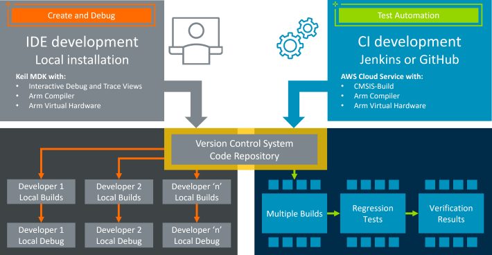 |
| The Arm Virtual Hardware end-to-end workflow, from developer to the cloud. |
GitHub Actions and Arm Virtual Hardware
GitHub Actions provides a popular CI solution for open-source projects, including TensorFlow Lite Micro. The AVH technology can be integrated with the GitHub Actions runner and that can be used to run tests on the different Arm platforms as natively compiled code without the need to have the hardware available.
Let’s get into how it’s done!
Defining a AVH use-case through a GitHub Actions workflow
Overview
Over the past year, we have made it possible to set up Arm IP verification in GitHub Actions. We will walk you through the steps needed to perform this integration with TFLM. The same process can be repeated for other open-source projects that use GitHub Actions as well.
A GitHub workflow file (such as Corstone-300 workflow in the TFLM repository) can be used to run code on an AWS EC2 instance, which has Arm IP installed. This workflow builds the TFLM project with Corstone-300 as a target, and runs the unit tests using both GCC and armclang, displaying the results directly in the GitHub UI via a hierarchical process as visualized below.
 |
The workflow contains one or more jobs, which points to a file containing steps. The steps are defined in a separate file (cortex_m_corstone_300_avh.yml). In our example, the steps will then point to a test script (test_cortex_m_corstone_300.sh), which is sent using an Arm-provided API (AVH Client) to the AWS instance where it is then executed accordingly. The script will send back output, which is obtained by the AVH client and can be displayed in the GitHub Actions UI.
Depending on the nature of the use case, this can happen one or several times, which all depends on the number of jobs and steps defined. In the Corstone-300 case, we use a single job with steps that will only run one test script only. This is not a limitation however, as visualized in the flowchart above.
Connecting the GitHub Actions runner to the AWS EC2 instance running AVH
Let’s have a look at how the AVH client connects to our AWS EC2 instance. The AVH client is a python-based tool that makes accessing AVH services easier. It sets up a VM which has the virtual hardware target (VHT) installed. The client can be installed from pypi.org using pip into any environment running Python. From there it can offload any compilation and test job onto Arm Virtual Hardware. For our Corstone-300 example, it is installed on the GitHub Actions runner by adding a pip install to the workflow file.
|
– name: Install AVH Client for Python
run: | |
The AWS credentials are configured to allow the AVH client to connect to the AWS EC2 instance, though there are various other ways to authenticate with AWS services. These include adding the AWS keypair onto GitHub secrets, or using an allow-listed GitHub repository to ordinate a predefined role, as shown here.
|
– name: Configure AWS Credentials |
Defining and executing a workload
Finally, let’s look at how the workload itself is executed using the AVH client. In this example, the AVH workload is described in a YAML file which we point to in the Github workflow file.
|
– name: Execute test suite on Arm Virtual Hardware at AWS |
This is where we define a list of steps to be executed. The steps will point to an inventory of files to be transferred, like the TFLM repository itself. Additionally, we define the code that we want to execute using these files, which can be done through the script that we provided earlier.
|
steps: |
Next, we set up a list of files to copy back to the GitHub Actions runner. For the TFLM unit test, a complete command line log will be written to a file, corstone300.log – that is returned to the GitHub Actions runner to analyze the test run outcome:
|
– name: Fetch results from Arm Virtual Hardware |
You can find a detailed explanation of avhclient and its usage on the Arm Virtual Hardware Client GitHub repository and the getting started guide.
Expanding the toolbox by adding more hardware targets
Using AVH it is easy to extend tests to all available Arm platforms. You can also avoid a negative impact on the overall CI workflow execution time by hosting through cloud services like AWS and spawning an arbitrary number of AVH instances in parallel.
Virtual Hardware targets like the Corstone-310 demonstrate how software validation is feasible even before silicon is available. This will make well-tested software stacks available for new Cortex-M devices from day one and we plan to expand the support. The introduction of Corstone-1000 will extend the range of tested architectures into the world of Cortex-A application processors, including Cortex-A32, Cortex-A35, Cortex-A53.
Wrapping up
To summarize: by providing a workflow file, a use-case file, and a workload (in our case, a test script), we have enabled running all the TFLM unit tests on the Corstone-300 and will work to extend it to all AVH targets available.
Thanks to the AVH integration, CI flows with virtual hardware targets open up new possibilities. Choosing the right architecture, integrating, and verifying has never been easier. We believe it is an important step in making embedded ML more accessible and that it will pave the way for future applications.
Thank you for reading!
Acknowledgements
We would like to acknowledge a number of our colleagues at Arm who have contributed to this project, including Samuel Peligrinello Caipers, Fredrik Knutsson, and Måns Nilsson.
We would also like to thank Advait Jain from Google and John Withers of Berkeley Design Technology, Inc. for architecting a continuous integration system using GitHub Actions that has enabled the Arm Virtual Hardware integration described in this article.
Keep On Trucking: SenSen Harnesses Drones, NVIDIA Jetson, Metropolis to Inspect Trucks
Sensor AI solutions specialist SenSen has turned to the NVIDIA Jetson edge AI platform to help regulators track heavy vehicles moving across Australia.
Australia’s National Heavy Vehicle Regulator, or NHVR, has a big job — ensuring the safety of truck drivers across some of the world’s most sparsely populated regions.
They’re now harnessing AI to improve safety and operational efficiency for the trucking industry — even as the trucks are on the move — using drones as well as compact, portable solar-powered trailers and automatic number-plate recognition cameras in the vehicle.
That’s a big change from current systems, which gather information after the fact, when it’s too late to use it to disrupt high-risk journeys and direct on-the-road compliance in real time.
Current license plate recognition systems are often fixed in place and can’t be moved to areas with the most traffic.
NHVR is developing and deploying real-time mobile cameras on multiple platforms to address this challenge, including vehicle-mounted, drone-mounted and roadside trailer-mounted systems.
The regulator turned to the Australia-based SenSen, an NVIDIA Metropolis partner, to build these systems for the pilot program, including two trailers, a pair of vehicles and a drone.
“SenSen technology helps the NHVR support affordable, adaptable and accurate road safety in Australia,” said Nathan Rogers, director of smart city solutions for Asia Pacific at SenSen.
NVIDIA Jetson helps SenSen create lightweight systems that have low energy needs and a small footprint, while being able to handle multiple camera streams integrated with lidar and inertial sensors. These systems operate solely on solar and battery power and are rapidly deployable.
NVIDIA technologies also play a vital role in the systems’ ability to intelligently analyze data fused from multiple cameras and sensors.
To train the AI application, SenSen relies on NVIDIA GPUs and the NVIDIA TAO Toolkit to fast-track the AI model development using transfer learning by refining the accuracy and optimizing the model performance to power the object-detection application.
To run the AI app, SenSen relies on the NVIDIA DeepStream software development kit for highly optimized video analysis in real time on NVIDIA Jetson Nano- and AGX Xavier-based systems.
These mobile systems promise to help safety and compliance officers identify and disrupt high-risk journeys real time.
This allows clients to get accurate data reliably and quickly identify operators who obey road rules, and to help policymakers make better decisions about road safety over the long term.
“Using this solution to obtain real-time heavy vehicle sightings from any location in Australia allows us to further digitize our operations and create a more efficient and safer heavy-vehicle industry in Australia,” said Paul Simionato, director of the southern region at NHVR.
The ultimate goal: waste less time tracking repeat compliant vehicles, present clearer information on vehicles and loads, and use vehicles as a mobile intelligence tool.
And perhaps best of all, operators who are consistently compliant can expect to be less regularly intercepted, creating a strong incentive for the industry to increase compliance.
The post Keep On Trucking: SenSen Harnesses Drones, NVIDIA Jetson, Metropolis to Inspect Trucks appeared first on NVIDIA Blog.
What Are Graph Neural Networks?
When two technologies converge, they can create something new and wonderful — like cellphones and browsers were fused to forge smartphones.
Today, developers are applying AI’s ability to find patterns to massive graph databases that store information about relationships among data points of all sorts. Together they produce a powerful new tool called graph neural networks.
What Are Graph Neural Networks?
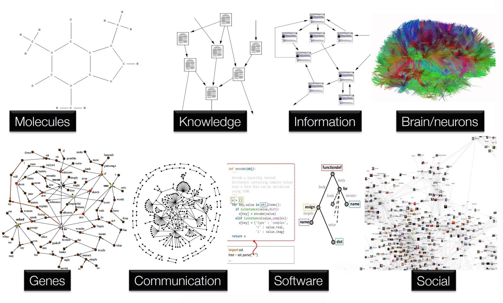
Graph neural networks apply the predictive power of deep learning to rich data structures that depict objects and their relationships as points connected by lines in a graph.
In GNNs, data points are called nodes, which are linked by lines — called edges — with elements expressed mathematically so machine learning algorithms can make useful predictions at the level of nodes, edges or entire graphs.
What Can GNNs Do?
An expanding list of companies is applying GNNs to improve drug discovery, fraud detection and recommendation systems. These applications and many more rely on finding patterns in relationships among data points.
Researchers are exploring use cases for GNNs in computer graphics, cybersecurity, genomics and materials science. A recent paper reported how GNNs used transportation maps as graphs to improve predictions of arrival time.
Many branches of science and industry already store valuable data in graph databases. With deep learning, they can train predictive models that unearth fresh insights from their graphs.
“GNNs are one of the hottest areas of deep learning research, and we see an increasing number of applications take advantage of GNNs to improve their performance,” said George Karypis, a senior principal scientist at AWS, in a talk earlier this year.
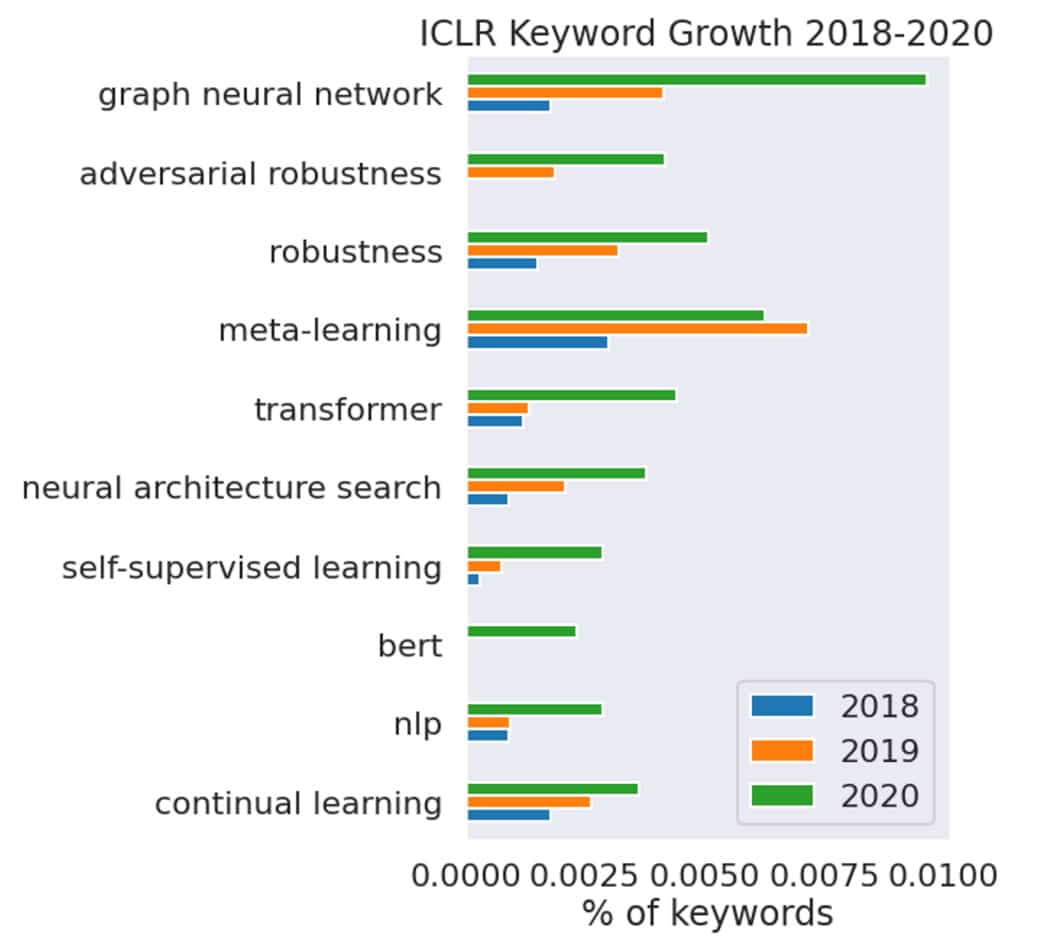
Others agree. GNNs are “catching fire because of their flexibility to model complex relationships, something traditional neural networks cannot do,” said Jure Leskovec, an associate professor at Stanford, speaking in a recent talk, where he showed the chart below of AI papers that mention them.
Who Uses Graph Neural Networks?
Amazon reported in 2017 on its work using GNNs to detect fraud. In 2020, it rolled out a public GNN service that others could use for fraud detection, recommendation systems and other applications.
To maintain their customers’ high level of trust, Amazon Search employs GNNs to detect malicious sellers, buyers and products. Using NVIDIA GPUs, it’s able to explore graphs with tens of millions of nodes and hundreds of millions of edges while reducing training time from 24 to five hours.
For its part, biopharma company GSK maintains a knowledge graph with nearly 500 billion nodes that is used in many of its machine-language models, said Kim Branson, the company’s global head of AI, speaking on a panel at a GNN workshop.
LinkedIn uses GNNs to make social recommendations and understand the relationships between people’s skills and their job titles, said Jaewon Yang, a senior staff software engineer at the company, speaking on another panel at the workshop.
“GNNs are general-purpose tools, and every year we discover a bunch of new apps for them,” said Joe Eaton, a distinguished engineer at NVIDIA who is leading a team applying accelerated computing to GNNs. “We haven’t even scratched the surface of what GNNs can do.”
In yet another sign of the interest in GNNs, videos of a course on them that Leskovec teaches at Stanford have received more than 700,000 views.
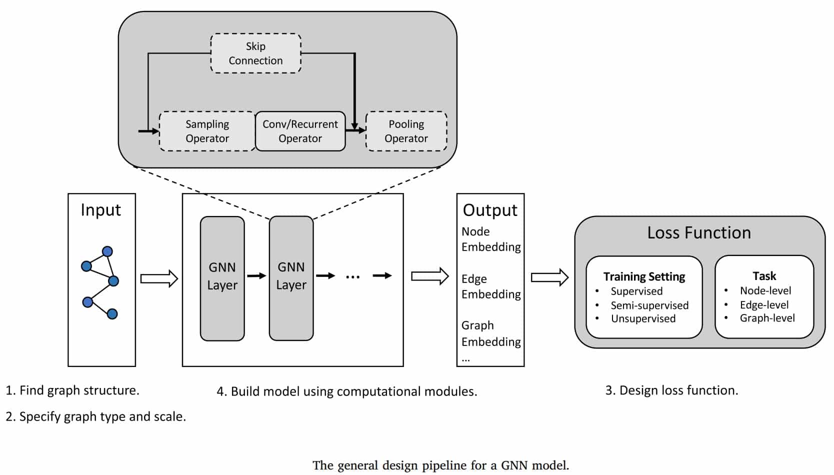
How Do GNNs Work?
To date, deep learning has mainly focused on images and text, types of structured data that can be described as sequences of words or grids of pixels. Graphs, by contrast, are unstructured. They can take any shape or size and contain any kind of data, including images and text.
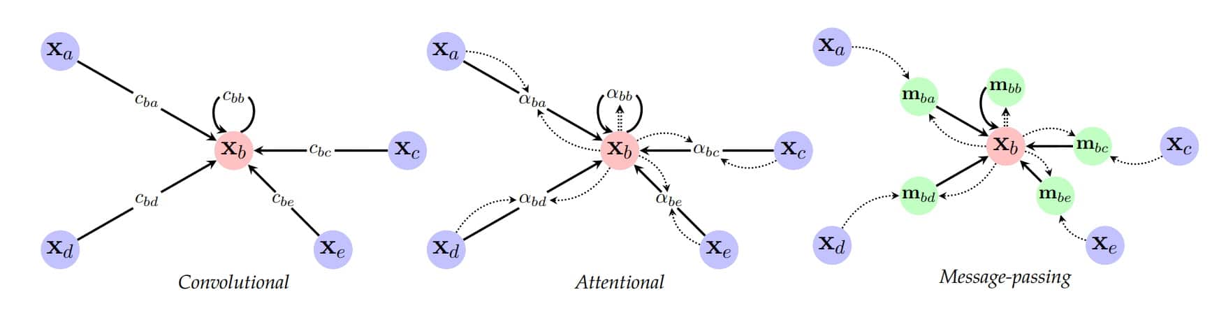
Using a process called message passing, GNNs organize graphs so machine learning algorithms can use them.
Message passing embeds into each node information about its neighbors. AI models employ the embedded information to find patterns and make predictions.
For example, recommendation systems use a form of node embedding in GNNs to match customers with products. Fraud detection systems use edge embeddings to find suspicious transactions, and drug discovery models compare entire graphs of molecules to find out how they react to each other.
GNNs are unique in two other ways: They use sparse math, and the models typically only have two or three layers. Other AI models generally use dense math and have hundreds of neural-network layers.
What’s the History of GNNs?
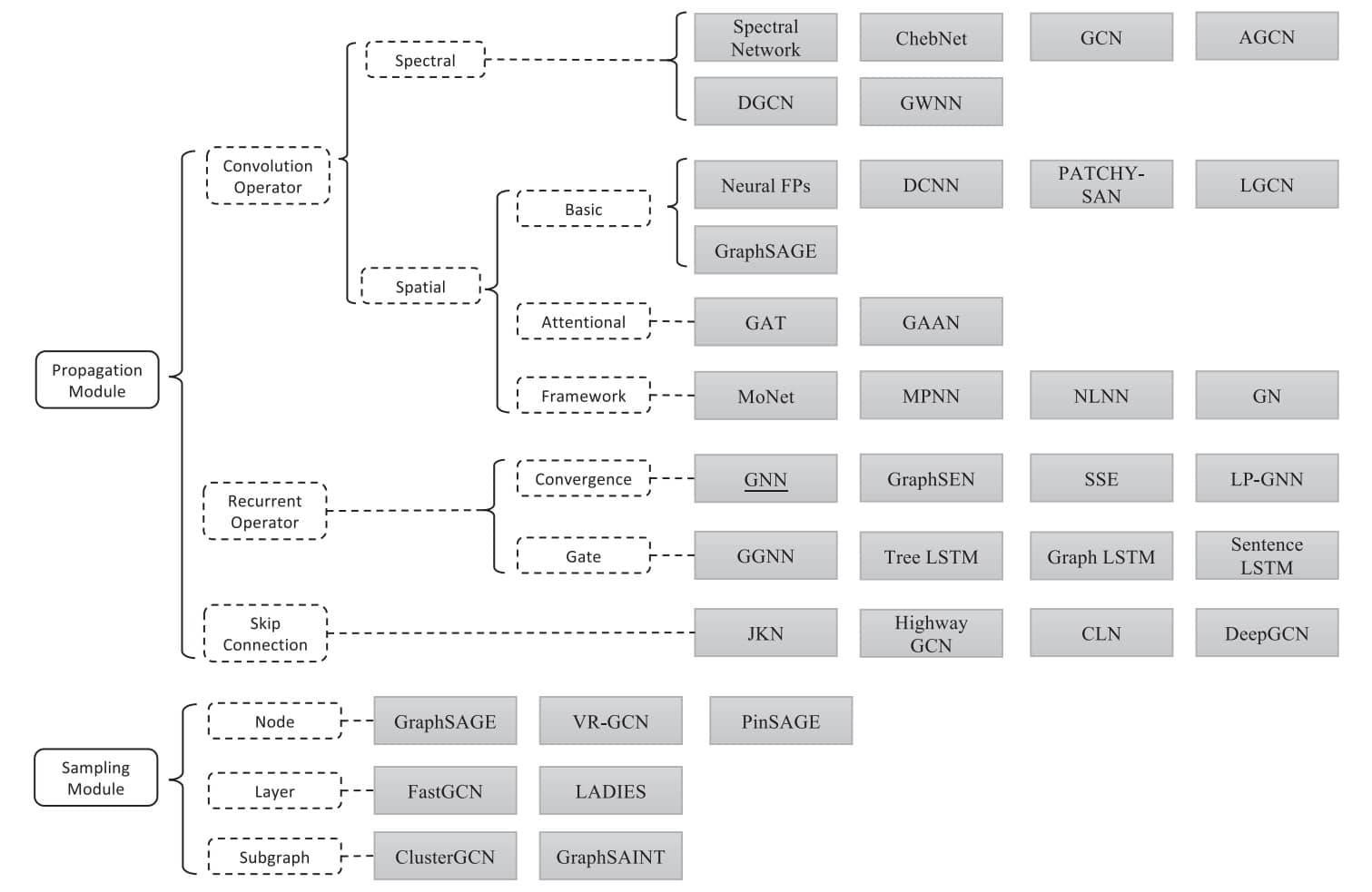
A 2009 paper from researchers in Italy was the first to give graph neural networks their name. But it took eight years before two researchers in Amsterdam demonstrated their power with a variant they called a graph convolutional network (GCN), which is one of the most popular GNNs today.
The GCN work inspired Leskovec and two of his Stanford grad students to create GraphSage, a GNN that showed new ways the message-passing function could work. He put it to the test in the summer of 2017 at Pinterest, where he served as chief scientist.
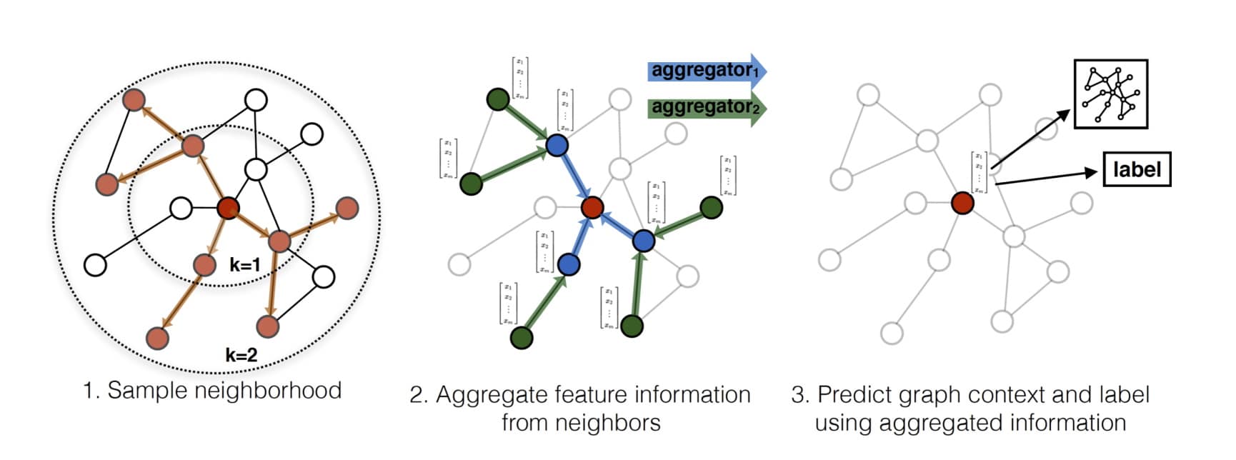
Their implementation, PinSage, was a recommendation system that packed 3 billion nodes and 18 billion edges to outperform other AI models at that time.
Pinterest applies it today on more than 100 use cases across the company. “Without GNNs, Pinterest would not be as engaging as it is today,” said Andrew Zhai, a senior machine learning engineer at the company, speaking on an online panel.
Meanwhile, other variants and hybrids have emerged, including graph recurrent networks and graph attention networks. GATs borrow the attention mechanism defined in transformer models to help GNNs focus on portions of datasets that are of greatest interest.
Scaling Graph Neural Networks
Looking forward, GNNs need to scale in all dimensions.
Organizations that don’t already maintain graph databases need tools to ease the job of creating these complex data structures.
Those who use graph databases know they’re growing in some cases to have thousands of features embedded on a single node or edge. That presents challenges of efficiently loading the massive datasets from storage subsystems through networks to processors.
“We’re delivering products that maximize the memory and computational bandwidth and throughput of accelerated systems to address these data loading and scaling issues,” said Eaton.
As part of that work, NVIDIA announced at GTC it is now supporting PyTorch Geometric (PyG) in addition to the Deep Graph Library (DGL). These are two of the most popular GNN software frameworks.
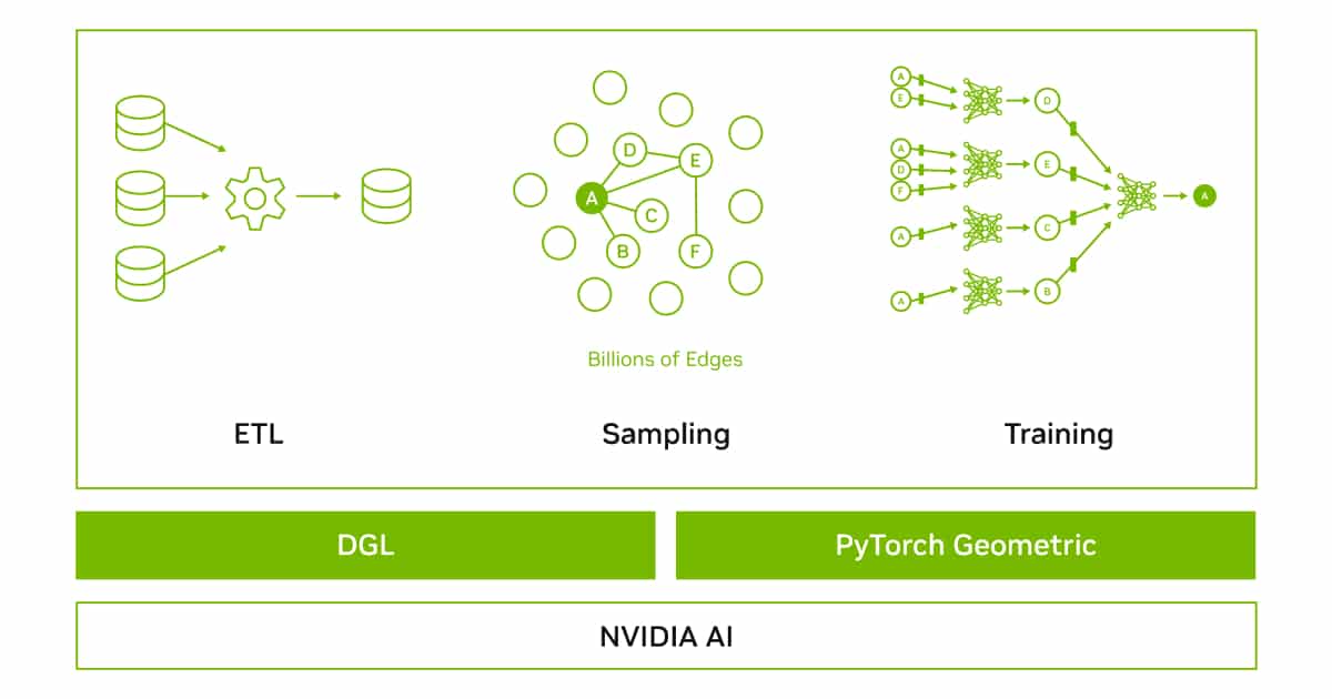
NVIDIA-optimized DGL and PyG containers are performance-tuned and tested for NVIDIA GPUs. They provide an easy place to start developing applications using GNNs.
To learn more, watch a talk on accelerating and scaling GNNs with DGL and GPUs by Da Zheng, a senior applied scientist at AWS. In addition, NVIDIA engineers hosted separate talks on accelerating GNNs with DGL and PyG.
To get started today, sign up for our early access program for DGL and PyG.
The post What Are Graph Neural Networks? appeared first on NVIDIA Blog.
The quest to deploy autonomous robots within Amazon fulfillment centers
Company is testing a new class of robots that use artificial intelligence and computer vision to move freely throughout facilities.Read More
ECCV 2022 highlights: Advancing the foundations of mixed reality
By Microsoft Mixed Reality & AI Labs in Cambridge and Zurich
Computer vision is one of the most remarkable developments to emerge from the field of computer science. It’s among the most rapidly growing areas in the technology landscape and has the potential to significantly impact the way people live and work. Advances at the intersection of machine learning (ML) and computer vision have been accelerating in recent years, leading to significant progress in numerous fields, including healthcare, robotics, the automotive industry, and augmented reality (AR). Microsoft is proud to be a prominent contributor to computer vision research.
Microsoft researchers have long been collaborating with academics and experts in the field on numerous computer vision projects with the goal of expanding what’s possible and helping people achieve more. One example is PeopleLens, a head-worn device that helps children who are blind or have low vision more easily interact in social situations by identifying people around them through spatialized audio. Another example is Swin Transformer. This computer vision architecture attains high accuracy in object detection and provides an opportunity to unify computer vision and natural language processing (NLP) architectures—increasing the capacity and adaptability of computer vision models.
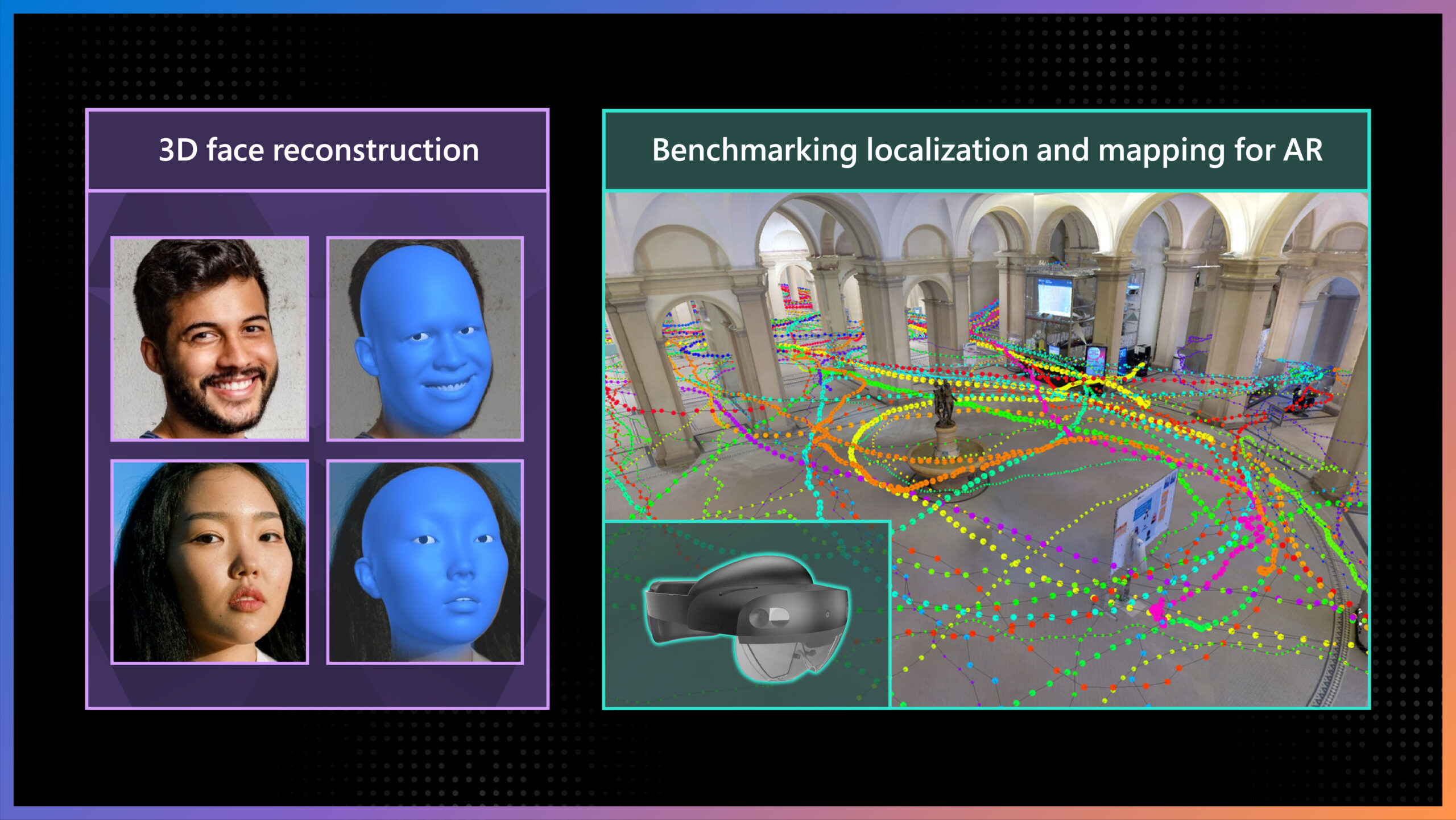
Microsoft Research is excited to share some of its newest work in this space at the European Conference on Computer Vision (ECCV) 2022, with 45 accepted papers that will be presented through live presentations, tutorials, and poster sessions. This post highlights two of these papers, which showcase the latest research from Microsoft and its collaborators. One involves increasing the number of facial landmarks for more accurate 3D face reconstruction, achieving state-of-the-art results while decreasing the required compute power. The other introduces a dataset that takes advantage of the capabilities of AR devices for visual localization and mapping driven by real-world AR scenarios.
3D face reconstruction with dense landmarks
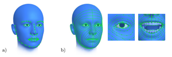
Facial landmarks are points that correspond across all faces, and they often play a key role in face analysis. Researchers frequently rely on them when performing basic computer vision tasks, such as estimating head position and identifying gaze direction and more generally the position in space of all the details of the face. Facial landmarks include such areas as the tip of the nose, corners of the eyes, and points along the jawline. Typically, public datasets that practitioners use to train ML models contain annotations for 68 facial landmarks. However, numerous aspects of human faces are not precisely represented by 68 landmarks alone, and additional methods are often needed to supplement landmark detection, adding complexity to the training workflow and increasing the required compute power.
-
GitHub
Dense Landmarks
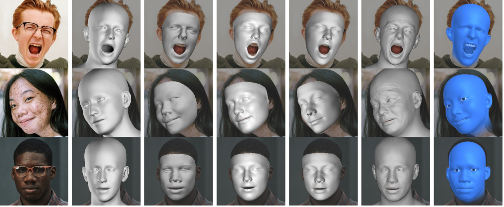
With the goal of achieving accurate 3D face reconstruction, we propose increasing the number of facial landmarks. In our paper “3D Face Reconstruction with Dense Landmarks,” we introduce a method to accurately predict 703 facial landmarks, more than 10 times as many as are commonly used, covering the entire face in great detail, including the eyes, ears, and teeth, as shown in Figure 1. We show that the increased number of landmarks are very precise when visible, and when they are occluded, for example, when someone lifts a coffee mug to their lips, we can estimate the location of these landmarks and what the part of the face looks like behind the object blocking it. We can use these landmarks to constrain a model-fitting problem to efficiently and precisely estimate all aspects of a face model, shown in the right-most column in Figure 2. This includes the head pose, eye gaze, as well as the identity of the person whose face is being reconstructed, for example, the thickness of the lips and the shape of the nose.
This simple pipeline is comprised only of dense landmarks and continuous mathematical optimization, allowing for extreme compute efficiency and enabling the entire system to run at over 150 frames per second on a single core of a laptop.
Increasing privacy, fairness, and efficiency with synthetic data
In computer vision, and particularly the area of face reconstruction, there are understandable concerns about anonymity when training ML models because training data often comes from real people. Our proposed method significantly reduces privacy concerns, as it uses only synthetic data to train ML models, compared with methods that use images of real people as part of their training datasets. That said, when we built the synthetic data pipeline, we needed to preserve the privacy of the people whose data we used, and we took care to acquire the consent of those several hundred subjects. This contrasts with the feasibility of acquiring consent from thousands (or even tens of thousands) of subjects, which would have been necessary if we were using real data.
It’s especially challenging, if not impossible, to preserve the privacy of people appearing in “found images” online, where the subject is often unknown. Using synthetic data helps us protect the privacy of data subjects and the rights of photographers and content creators. It’s another tool we can use in our mission to build technology in an ethical and responsible manner. Additionally, because people’s private information is not included in our dataset, if the ML model were to be attacked, only synthetic data would be subject to compromise.
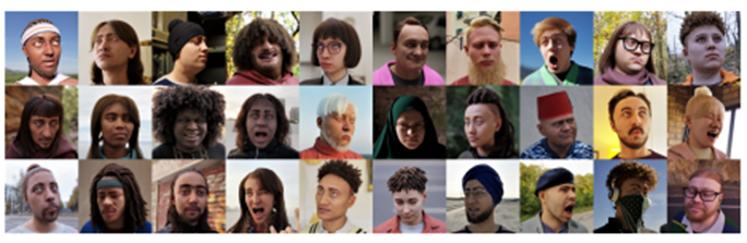
Synthetic data also provides an opportunity to address inclusivity and fairness. Largely because the distribution of the data is fully controlled, ML practitioners can manage the fairness of representation by including diverse samples in their datasets, and all the data needed to do this would be perfectly labeled. For further details on how we build the synthetics model and training data and our approach to capturing the diversity of the human population, please see our face analysis paper.
There are other advantages to using synthetic data to train ML models, as well. For example, these models require a lot of data, giving rise to numerous difficulties that practitioners must navigate to obtain this data, such as the logistics of finding the number of people required, scheduling time in a lab, and situating multiple cameras to capture the various angles of a person’s face. These concerns are greatly reduced with synthetic data.
In addition, because data doesn’t need to be sourced from a real person, the iteration speed to improve the quality of the 3D face reconstruction is remarkably high, creating a robust workflow. And it isn’t necessary to apply quality assurance (QA) processes on each labeled image when using synthetic data—another cost- and time-saving benefit. Another advantage is the increase in accuracy, speed, and cost-effectiveness in labeling data. It would be nearly impossible to ask someone to consistently label 703 landmarks in a set of images.
Face analysis is a foundational piece for many ML systems, such as facial recognition and controlling avatars, and using a method that provides both accuracy and efficiency while also addressing privacy and fairness concerns pushes the boundaries of the state of the art. Up until now, there hasn’t been much work, if any, on methods that can yield this level of quality with only synthetic data. The ability to achieve 3D face reconstruction using dense landmarks and synthetic data has the potential to truly transform what’s possible with ML.
Acknowledgments
This research was conducted by Erroll Wood, Tadas Baltrušaitis, Charlie Hewitt, Matthew Johnson, Jingjing Shen, Nikola Milosavljević, Daniel Wilde, Stephan Garbin, Chirag Raman, Jamie Shotton, Toby Sharp, Ivan Stojiljković, Tom Cashman, and Julien Valentin.
LaMAR: Benchmarking localization and mapping for augmented reality
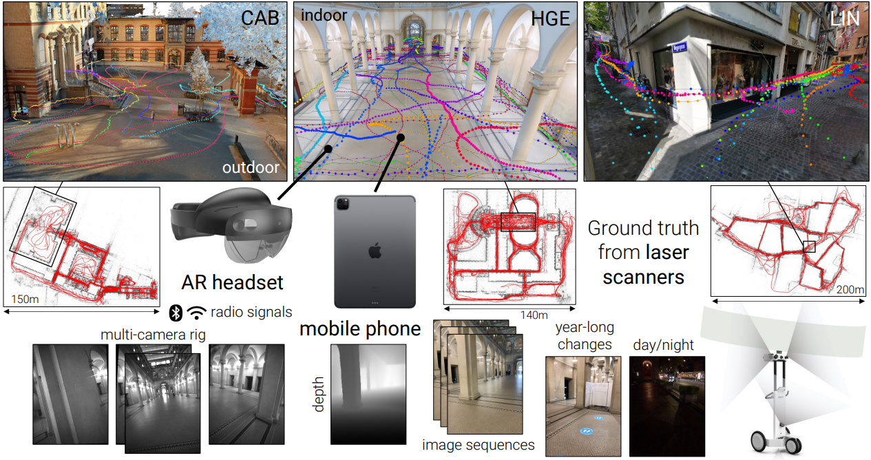
To unlock the full potential of augmented reality (AR), anyone using a mixed reality headset should be able to place virtual content in the physical world, share it with others, and expect it to remain in place over time. However, before they can augment digital content in the real world in the form of holograms, AR devices need to build a digital map of the physical 3D world. These devices then position, or re-localize, themselves with respect to this map, as illustrated in Figure 4, which allows them to retrieve previously placed holograms and show them to the user at a designated location. The computer vision foundations enabling these capabilities are called mapping and visual localization.
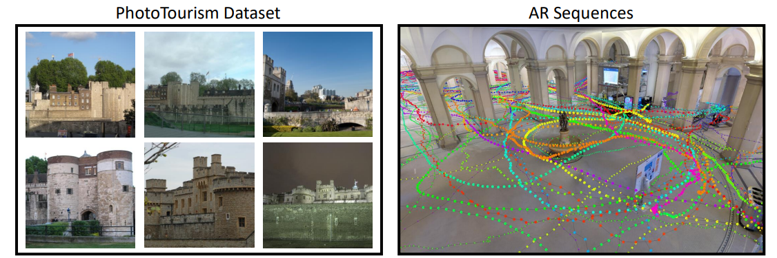
In general, research in visual localization focuses on single images, usually carefully selected views of famous attractions, shown on the left in Figure 5. However, this doesn’t reflect real AR scenarios—the combination of AR devices and applications—and the opportunity they provide. AR devices can locally map the environment and provide spatially registered sequences rather than single images, as shown in the image on the right in Figure 5. These sequences can also include additional data, like inertial or radio signals from sensors, which are typically available on modern AR devices, such as Microsoft HoloLens 2. Yet it’s challenging to use such sequences for localization because they are typically just collected during normal device usage and not generally aimed at facilitating localization.
To close this gap, we introduce a new benchmark, the first to focus on this more realistic setting for AR, with the understanding that visual re-localization is a key element for compelling, shared, and persistent AR experiences. Given the spatial scale of the environment for typical AR scenarios, such as navigating an airport or inspecting a factory, we had to design a pipeline that could automatically compute the ground-truth camera positions of real AR sequences captured by a variety of readily available AR devices, such as the HoloLens or iPhone. By evaluating state-of-the-art methods on our benchmark, we offer novel insights on current research and provide avenues for future work in the field of visual localization and mapping for AR.
This research is a result of a two-year collaboration between the Microsoft Mixed Reality & AI Lab in Zurich and ETH Zurich (Swiss Federal Institute of Technology) and will be published at ECCV 2022 in the paper, “LaMAR: Benchmarking Localization and Mapping for Augmented Reality.” We will also be giving a tutorial called Localization and Mapping for AR at ECCV.
Developing a large-scale AR dataset
To enable the research community to address the specifics of mapping and visual localization in the context of AR, we collected multi-sensor data streams from modern AR devices. These sensor streams come with camera poses (the camera’s position and orientation) from the on-device tracker at each instant. These data streams also contain images, depth measurements, samples from inertial measurement units (IMUs), and radio signals. Exploiting these can lead to more efficient algorithms. For example, radio signals such as Wi-Fi or Bluetooth can simplify image retrieval. Similarly, sequence localization can exploit the temporal aspect of sensor streams to provide a more spatial context, which can lead to more accurate estimates of camera poses. This typifies the realistic use case of a user launching an AR application and streaming sensorial data to localize the camera with respect to a previously built map, and it reflects how AR applications built on mixed reality cloud services, like Azure Spatial Anchors, work.
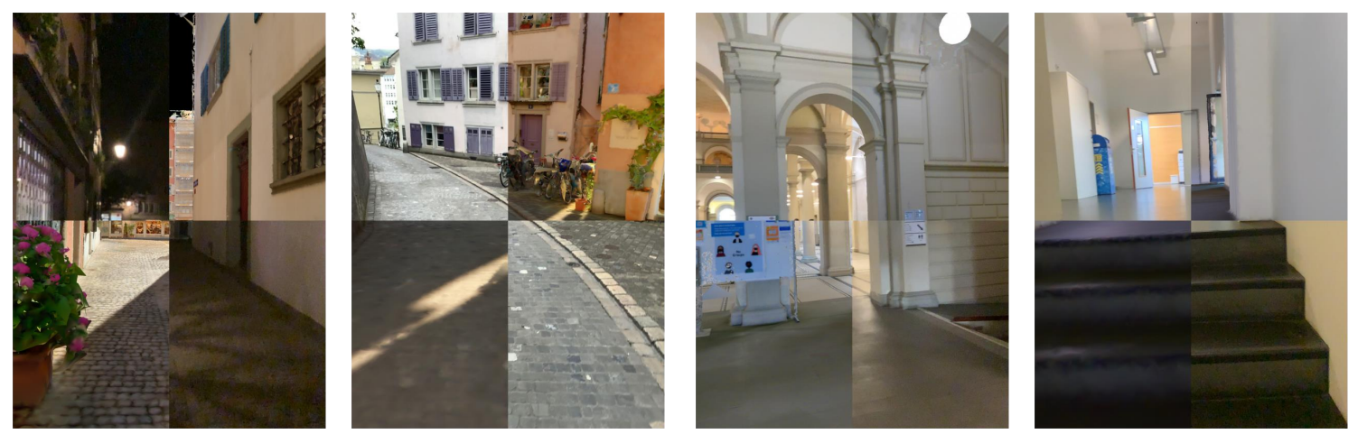
The initial release of the LaMAR dataset contains more than 100 hours of recordings covering 45,000 square meters (484,000 square feet) captured over the course of two years using the head-mounted HoloLens 2 and handheld iPhone/iPad devices. The data was captured at various indoor and outdoor locations (a historical building, a multi-story office building, and part of a city center) and represents typical AR scenarios. It includes changes in illumination and the movement of objects—either slowly, such as the placement of a book on a desk, or more quickly, like anonymized people walking down a sidewalk.
Automatically aligning AR sequences to establish ground truth
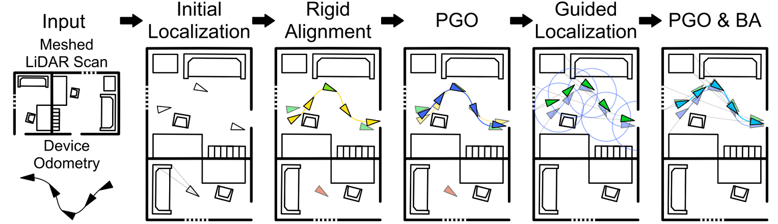
To estimate the ground-truth camera poses, we aligned the captured data with reference 3D models of the locations, as shown in Figure 8. These reference models were captured using NavVis M6 and VLX mapping systems, both equipped with laser scanners (lidars) that generate dense, textured, and highly accurate 3D models of the locations. To align the data, we developed a robust pipeline that does not require manual labeling or setting custom infrastructure, such as fiducial markers, and this enabled us to robustly handle crowd-sourced data from a variety of AR devices captured over extended periods.
The actual alignment process is fully automatic and utilizes the on-device real-time tracker of AR devices, which provides camera poses in their local coordinate system. We aligned each captured sequence individually with the dense ground truth reference model, as illustrated in Figure 9. Once completed, all camera poses were refined jointly by optimizing the visual constraints within and across sequences.
Evaluating localization and mapping in the context of AR
We evaluated current state-of-the-art approaches in the single-frame setting as localizing i) single images obtained from phones and ii) single images and full camera rigs from HoloLens 2. Then we adapted these state-of-the-art approaches to take advantage of radio signals. Finally, we designed baselines, building on these methods and utilizing the on-device real-time tracker in a multi-frame localization setting corresponding to a real-world AR application. The results show that performance of state-of-the-art methods can be significantly improved by including these additional data streams generally available in modern AR devices, as shown in Figure 10.
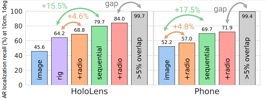
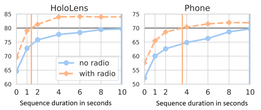
For a compelling user experience, AR applications should strive to retrieve and visualize content as quickly as possible after starting a session. To quantify this, we introduce a new metric called time-to-recall, which measures the sequence duration needed for successful localization. This encourages researchers to develop algorithms to accurately localize the camera as quickly as possible, as shown in Figure 11.
Using the LaMAR benchmark
LaMAR is the first benchmark that focuses on a realistic setup for visual localization and mapping using AR devices. The evaluation results show enormous potential for leveraging posed sequences instead of single frames and for leveraging other sensor modalities, like radio signals, to localize the camera and map the environment.
Researchers can access the LaMAR benchmark, evaluation server, implementations of the ground-truth pipeline, as well as baselines with additional sensory data at the LaMAR Benchmark page. We hope this work inspires future research in developing localization and mapping algorithms tailored to real AR scenarios.
Acknowledgments
This research was conducted by Paul-Edouard Sarlin, Mihai Dusmanu, Johannes L. Schönberger, Pablo Speciale, Lukas Gruber, Viktor Larsson, Ondrej Miksik, and Marc Pollefeys.
The post ECCV 2022 highlights: Advancing the foundations of mixed reality appeared first on Microsoft Research.
Q&A with Akshitha Sriraman, Assistant Professor, Department of Electrical and Computer Engineering, Carnegie Mellon University
For October, we are spotlighting Akshitha Sriraman, Assistant Professor, Department of Electrical and Computer Engineering at Carnegie Mellon University (CMU).Read More