Monthly Archives: December 2022

Amazon SageMaker JumpStart is the Machine Learning (ML) hub of SageMaker providing pre-trained, publicly available models for a wide range of problem types to help you get started with machine learning.

JumpStart also offers example notebooks that use Amazon SageMaker features like spot instance training and experiments over a large variety of model types and use cases. These example notebooks contain code that shows how to apply ML solutions by using SageMaker and JumpStart. They can be adapted to match to your own needs and can thus speed up application development.

Recently, we added 10 new notebooks to JumpStart in Amazon SageMaker Studio. This post focuses on these new notebooks. As of this writing, JumpStart offers 56 notebooks, ranging from using state-of-the-art natural language processing (NLP) models to fixing bias in datasets when training models.

The 10 new notebooks can help you in the following ways:

• They offer example code for you to run as is from the JumpStart UI in Studio and see how the code works
• They show the usage of various SageMaker and JumpStart APIs
• They offer a technical solution that you can further customize based on your own needs

The number of notebooks that are offered through JumpStart increase on a regular basis as more notebooks are added. These notebooks are also available on github.

Notebooks overview

The 10 new notebooks are as follows:

• In-context learning with AlexaTM 20B – Demonstrates how to use AlexaTM 20B for in-context learning with zero-shot and few-shot learning on five example tasks: text summarization, natural language generation, machine translation, extractive question answering, and natural language inference and classification.
• Fairness linear learner in SageMaker – There have recently been concerns about bias in ML algorithms as a result of mimicking existing human prejudices. This notebook applies fairness concepts to adjust model predictions appropriately.
• Manage ML experimentation using SageMaker Search – Amazon SageMaker Search lets you quickly find and evaluate the most relevant model training runs from potentially hundreds and thousands of SageMaker model training jobs.
• SageMaker Neural Topic Model – SageMaker Neural Topic Model (NTM) is an unsupervised learning algorithm that attempts to describe a set of observations as a mixture of distinct categories.
• Predict driving speed violations – The SageMaker DeepAR algorithm can be used to train a model for multiple streets simultaneously, and predict violations for multiple street cameras.
• Breast cancer prediction – This notebook uses UCI’S breast cancer diagnostic dataset to build a predictive model of whether a breast mass image indicates a benign or malignant tumor.
• Ensemble predictions from multiple models – By combining or averaging predictions from multiple sources and models, we typically get an improved forecast. This notebook illustrates this concept.
• SageMaker asynchronous inference – Asynchronous inference is a new inference option for near-real-time inference needs. Requests can take up to 15 minutes to process and have payload sizes of up to 1 GB.
• TensorFlow bring your own model – Learn how to train a TensorFlow model locally and deploy on SageMaker using this notebook.
• Scikit-learn bring your own model – This notebook shows how to use a pre-trained Scikit-learn model with the SageMaker Scikit-learn container to quickly create a hosted endpoint for that model.

Prerequisites

To use these notebooks, make sure that you have access to Studio with an execution role that allows you to run SageMaker functionality.  The short video below will help you navigate to JumpStart notebooks.

In the following sections, we go through each of the 10 new solutions and discuss some of their interesting details.

In-context learning with AlexaTM 20B

AlexaTM 20B is a multitask, multilingual, large-scale sequence-to-sequence (seq2seq) model, trained on a mixture of Common Crawl (mC4) and Wikipedia data across 12 languages, using denoising and Causal Language Modeling (CLM) tasks. It achieves state-of-the-art performance on common in-context language tasks such as one-shot summarization and one-shot machine translation, outperforming decoder only models such as Open AI’s GPT3 and Google’s PaLM, which are over eight times bigger.

In-context learning, also known as prompting, refers to a method where you use an NLP model on a new task without having to fine-tune it. A few task examples are provided to the model only as part of the inference input, a paradigm known as few-shot in-context learning. In some cases, the model can perform well without any training data at all, only given an explanation of what should be predicted. This is called zero-shot in-context learning.

This notebook demonstrates how to deploy AlexaTM 20B through the JumpStart API and run inference. It also demonstrates how AlexaTM 20B can be used for in-context learning with five example tasks: text summarization, natural language generation, machine translation, extractive question answering, and natural language inference and classification.

The notebook demonstrates the following:

• One-shot text summarization, natural language generation, and machine translation using a single training example for each of these tasks
• Zero-shot question answering and natural language inference plus classification using the model as is, without the need to provide any training examples.

Try running your own text against this model and see how it summarizes text, extracts Q&A, or translates from one language to another.

Fairness linear learner in SageMaker

There have recently been concerns about bias in ML algorithms as a result of mimicking existing human prejudices. Nowadays, several ML methods have strong social implications, for example they are used to predict bank loans, insurance rates, or advertising. Unfortunately, an algorithm that learns from historical data will naturally inherit past biases. This notebook presents how to overcome this problem by using SageMaker and fair algorithms in the context of linear learners.

It starts by introducing some of the concepts and math behind fairness, then it downloads data, trains a model, and finally applies fairness concepts to adjust model predictions appropriately.

The notebook demonstrates the following:

• Running a standard linear model on UCI’s Adult dataset.
• Showing unfairness in model predictions
• Fixing data to remove bias
• Retraining the model

Try running your own data using this example code and detect if there is bias. After that, try removing bias, if any, in your dataset using the provided functions in this example notebook.

Manage ML experimentation using SageMaker Search

SageMaker Search lets you quickly find and evaluate the most relevant model training runs from potentially hundreds and thousands of SageMaker model training jobs. Developing an ML model requires continuous experimentation, trying new learning algorithms, and tuning hyperparameters, all while observing the impact of such changes on model performance and accuracy. This iterative exercise often leads to an explosion of hundreds of model training experiments and model versions, slowing down the convergence and discovery of a winning model. In addition, the information explosion makes it very hard down the line to trace back the lineage of a model version—the unique combination of datasets, algorithms, and parameters that brewed that model in the first place.

This notebook shows how to use SageMaker Search to quickly and easily organize, track, and evaluate your model training jobs on SageMaker. You can search on all the defining attributes from the learning algorithm used, hyperparameter settings, training datasets used, and even the tags you have added on the model training jobs. You can also quickly compare and rank your training runs based on their performance metrics, such as training loss and validation accuracy, thereby creating leaderboards for identifying the winning models that can be deployed into production environments. SageMaker Search can quickly trace back the complete lineage of a model version deployed in a live environment, right up until the datasets used in training and validating the model.

The notebook demonstrates the following:

• Training a linear model three times
• Using SageMaker Search to organize and evaluate these experiments
• Visualizing the results in a leaderboard
• Deploying a model to an endpoint
• Tracing lineage of the model starting from the endpoint

In your own development of predictive models, you may be running several experiments. Try using SageMaker Search in such experiments and experience how it can help you in multiple ways.

SageMaker Neural Topic Model

SageMaker Neural Topic Model (NTM) is an unsupervised learning algorithm that attempts to describe a set of observations as a mixture of distinct categories. NTM is most commonly used to discover a user-specified number of topics shared by documents within a text corpus. Here each observation is a document, the features are the presence (or occurrence count) of each word, and the categories are the topics. Because the method is unsupervised, the topics aren’t specified up-front and aren’t guaranteed to align with how a human may naturally categorize documents. The topics are learned as a probability distribution over the words that occur in each document. Each document, in turn, is described as a mixture of topics.

This notebook uses the SageMaker NTM algorithm to train a model on the 20NewsGroups dataset. This dataset has been widely used as a topic modeling benchmark.

The notebook demonstrates the following:

• Creating a SageMaker training job on a dataset to produce an NTM model
• Using the model to perform inference with a SageMaker endpoint
• Exploring the trained model and visualizing learned topics

You can easily modify this notebook to run on your text documents and divide them into various topics.

Predict driving speed violations

This notebook demonstrates time series forecasting using the SageMaker DeepAR algorithm by analyzing the city of Chicago’s Speed Camera Violation dataset. The dataset is hosted by Data.gov, and is managed by the U.S. General Services Administration, Technology Transformation Service.

These violations are captured by camera systems and are available to improve the lives of the public through the city of Chicago data portal. The Speed Camera Violation dataset can be used to discern patterns in the data and gain meaningful insights.

The dataset contains multiple camera locations and daily violation counts. Each daily violation count for a camera can be considered a separate time series. You can use the SageMaker DeepAR algorithm to train a model for multiple streets simultaneously, and predict violations for multiple street cameras.

The notebook demonstrates the following:

• Training the SageMaker DeepAR algorithm on the time series dataset using spot instances
• Making inferences on the trained model to make traffic violation predictions

With this notebook, you can learn how time series problems can be solved using the DeepAR algorithm in SageMaker and try applying it on your own time series datasets.

Breast cancer prediction

This notebook takes an example for breast cancer prediction using UCI’S breast cancer diagnostic dataset. It uses this dataset to build a predictive model of whether a breast mass image indicates a benign or malignant tumor.

The notebook demonstrates the following:

• Basic setup for using SageMaker
• Converting datasets to Protobuf format used by the SageMaker algorithms and uploading to Amazon Simple Storage Service (Amazon S3)
• Training a SageMaker linear learner model on the dataset
• Hosting the trained model
• Scoring using the trained model

You can go through this notebook to learn how to solve a business problem using SageMaker, and understand the steps involved for training and hosting a model.

Ensemble predictions from multiple models

In practical applications of ML on predictive tasks, one model often doesn’t suffice. Most prediction competitions typically require combining forecasts from multiple sources to get an improved forecast. By combining or averaging predictions from multiple sources or models, we typically get an improved forecast. This happens because there is considerable uncertainty in the choice of the model and there is no one true model in many practical applications. Therefore, it’s beneficial to combine predictions from different models. In the Bayesian literature, this idea is referred to as Bayesian model averaging, and has been shown to work much better than just picking one model.

This notebook presents an illustrative example to predict if a person makes over $50,000 a year based on information about their education, work experience, gender, and more.

The notebook demonstrates the following:

• Preparing your SageMaker notebook
• Loading a dataset from Amazon S3 using SageMaker
• Investigating and transforming the data so that it can be fed to SageMaker algorithms
• Estimating a model using the SageMaker XGBoost (Extreme Gradient Boosting) algorithm
• Hosting the model on SageMaker to make ongoing predictions
• Estimating a second model using the SageMaker linear learner method
• Combining the predictions from both models and evaluating the combined prediction
• Generating final predictions on the test dataset

Try running this notebook on your dataset and using multiple algorithms. Try experimenting with various combination of models offered by SageMaker and JumpStart and see which combination of model ensembling gives the best results on your own data.

SageMaker asynchronous inference

SageMaker asynchronous inference is a new capability in SageMaker that queues incoming requests and processes them asynchronously. SageMaker currently offers two inference options for customers to deploy ML models: a real-time option for low-latency workloads, and batch transform, an offline option to process inference requests on batches of data available up-front. Real-time inference is suited for workloads with payload sizes of less than 6 MB and require inference requests to be processed within 60 seconds. Batch transform is suitable for offline inference on batches of data.

Asynchronous inference is a new inference option for near-real-time inference needs. Requests can take up to 15 minutes to process and have payload sizes of up to 1 GB. Asynchronous inference is suitable for workloads that don’t have subsecond latency requirements and have relaxed latency requirements. For example, you might need to process an inference on a large image of several MBs within 5 minutes. In addition, asynchronous inference endpoints let you control costs by scaling down endpoint instance count to zero when they’re idle, so you only pay when your endpoints are processing requests.

The notebook demonstrates the following:

• Creating a SageMaker model
• Creating an endpoint using this model and asynchronous inference configuration
• Making predictions against this asynchronous endpoint

This notebook shows you a working example of putting together an asynchronous endpoint for a SageMaker model.

TensorFlow bring your own model

A TensorFlow model is trained locally on a classification task where this notebook is being run. Then it’s deployed on a SageMaker endpoint.

The notebook demonstrates the following:

• Training a TensorFlow model locally on the IRIS dataset
• Importing that model into SageMaker
• Hosting it on an endpoint

If you have TensorFlow models that you developed yourself, this example notebook can help you host your model on a SageMaker managed endpoint.

Scikit-learn bring your own model

SageMaker includes functionality to support a hosted notebook environment, distributed, serverless training, and real-time hosting. It works best when all three of these services are used together, but they can also be used independently. Some use cases may only require hosting. Maybe the model was trained prior to SageMaker existing, in a different service.

The notebook demonstrates the following:

• Using a pre-trained Scikit-learn model with the SageMaker Scikit-learn container to quickly create a hosted endpoint for that model

If you have Scikit-learn models that you developed yourself, this example notebook can help you host your model on a SageMaker managed endpoint.

Clean up resources

After you’re done running a notebook in JumpStart, make sure to Delete all resources so that all the resources that you created in the process are deleted and your billing is stopped. The last cell in these notebooks usually deletes endpoints that are created.

Summary

This post walked you through 10 new example notebooks that were recently added to JumpStart. Although this post focused on these 10 new notebooks, there are a total of 56 available notebooks as of this writing. We encourage you to log in to Studio and explore the JumpStart notebooks yourselves, and start deriving immediate value out of them. For more information, refer to Amazon SageMaker Studio and SageMaker JumpStart.

About the Author

Dr. Raju Penmatcha is an AI/ML Specialist Solutions Architect in AI Platforms at AWS. He received his PhD from Stanford University. He works closely on the low/no-code suite services in SageMaker that help customers easily build and deploy machine learning models and solutions.

Read More

According to a 2020 survey of data scientists conducted by Anaconda, data preparation is one of the critical steps in machine learning (ML) and data analytics workflows, and often very time consuming for data scientists. Data scientists spend about 66% of their time on data preparation and analysis tasks, including loading (19%), cleaning (26%), and visualizing data (21%).

Amazon SageMaker Studio is the first fully integrated development environment (IDE) for ML. With a single click, data scientists and developers can quickly spin up Studio notebooks to explore datasets and build models. If you prefer a GUI-based and interactive interface, you can use Amazon SageMaker Data Wrangler, with over 300 built in visualizations, analyses, and transformations to efficiently process data backed by Spark without writing a single line of code.

Data Wrangler now offers a built-in data preparation capability in Amazon SageMaker Studio Notebooks that allows ML practitioners to visually review data characteristics, identify issues, and remediate data-quality problems—in just a few clicks directly within the notebooks.

In this post, we show you how the Data Wrangler data prep widget automatically generates key visualizations on top of a Pandas data frame to understand data distribution, detect data quality issues, and surface data insights such as outliers for each feature. It helps interact with the data and discover insights that may go unnoticed with ad hoc querying. It also recommends transformations to remediate, enables you to apply data transformations on the UI and automatically generate code in the notebook cells. This feature is available in all regions where SageMaker Studio is available.

Solution overview

Let’s further understand how this new widget makes data exploration significantly easier and provides a seamless experience to improve the overall data preparation experience for data engineers and practitioners. For our use case, we use of a modified version of the Titanic dataset, a popular dataset in the ML community, which has now been added as a sample dataset so you can get started with SageMaker Data Wrangler quickly. The original dataset was obtained from OpenML, and modified to add synthetic data quality issues by Amazon for this demo. You can download the modified version of dataset from public S3 path s3://sagemaker-sample-files/datasets/tabular/dirty-titanic/titanic-dirty-4.csv.

Prerequisites

To get hands-on experience with all the features described in this post, complete the following prerequisites:

1. Ensure that you have an AWS account, secure access to log in to the account via the AWS Management Console, and AWS Identity and Access Management (IAM) permissions to use Amazon SageMaker and Amazon Simple Storage Service (Amazon S3) resources.
2. Use the sample dataset from public S3 path s3://sagemaker-sample-files/datasets/tabular/dirty-titanic/titanic-dirty-4.csv or alternatively upload it to an S3 bucket in your account.
3. Onboard to a SageMaker domain and access Studio to use notebooks. For instructions, refer to Onboard to Amazon SageMaker Domain. If you’re using existing Studio, upgrade to the latest version of Studio.

Enable the data exploration widget

When you’re using Pandas data frames, Studio notebook users can manually enable the data exploration widget so that new visualizations are displayed by default on top of each column. The widget shows a histogram for numerical data and a bar chart for other types of data. These representations allow you to quickly comprehend the data distribution and discover missing values and outliers without having to write boilerplate methods for each and every column. You can hover over the bar in each visual to get a quick understanding of the distribution.

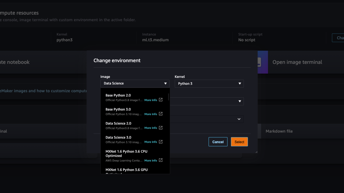
Open Studio and create a new Python 3 notebook. Make sure to choose the Data Science 3.0 image from SageMaker images by clicking Change environment button.

The data exploration widget is available in the following images. For the list of default SageMaker images, refer to Available Amazon SageMaker Images.

• Python 3 (Data Science) with Python 3.7
• Python 3 (Data Science 2.0) with Python 3.8
• Python 3 (Data Science 3.0) with Python 3.10
• Spark Analytics 1.0 and 2.0

To use this widget, import the SageMaker_DataWrangler library. Load the modified version of the Titanic dataset from S3://sagemaker-sample-files/datasets/tabular/dirty-titanic/titanic-dirty-4.csv and read the CSV with the Pandas library:

import pandas as pd
import boto3
import io
import sagemaker_datawrangler

s3 = boto3.client('s3')
obj = s3.get_object(Bucket='sagemaker-sample-files', Key='datasets/tabular/dirty-titanic/titanic-dirty-4.csv')
df = pd.read_csv(io.BytesIO(obj['Body'].read()))

Visualize the data

After the data is loaded in the Pandas data frame, you can view the data by just using df or display(df). Along with listing the row, the data prep widget produces insights, visualizations, and advice on data quality. You don’t need to write any additional code to generate feature and target insights, distribution information, or rendering data quality checks. You can choose the data frame table’s header to view the statistical summary showing the data quality warnings, if any.

Each column shows a bar chart or histogram based on the data type. By default, the widget samples up to 10,000 observations for generating meaningful insights. It also provides the option to run the insight analysis on the entire dataset.

As shown in the following screenshot, this widget identifies whether a column has categorical or quantitative data.

For categorical data, the widget generates the bar chart with all the categories. In the following screenshot, for example, the column Sex identifies the categories on the data. You can hover over the bar (male in this case) to see the details of these categories, like the total number of rows with the value male and its distribution in the total visualized dataset (64.07% in this example). It also highlights the total percentage of missing values in a different color for categorical data. For quantitative data like the ticket column, it shows distribution along with the percentage of invalid values.

If you want to see a standard Pandas visualization in the notebook, you can choose View the Pandas table and toggle between the widget and the Pandas representation, as shown in the following screenshot.

To get more detailed insights about the data in the column, choose the column’s header to open a side panel dedicated to the column. Here you can observe two tabs: Insights and Data quality.

In the following sections, we explore these two options in more detail.

Insights

The Insights tab provides details with descriptions for each column. This section lists aggregated statistics, such as mode, number of uniques, ratios and counts for missing/invalid values, etc., as well as visualize data distribution with help of a histogram or a bar chart. In the following screenshots, you can check out the data insights and distribution information displayed with easily understandable visualizations generated for the selected column survived.

Data quality

The studio data prep widget highlights identified data quality issues with the warning sign in the header. Widget can identify the whole spectrum of data quality issues from basics (missing values, constant column, etc.) to more ML specific (target leakage, low predictive score features, etc.). Widget highlights the cells causing the data quality issue and reorganize the rows to put the problematic cells at the top. To remedy the data quality issue widget provides several transformers, applicable on a click of a button.

To explore the data quality section, choose the column header, and in the side panel, choose the Data quality tab. You should see the following in your Studio environment.

Let’s look at the different options available on the Data quality tab. For this example, we choose the age column, which is detected as a quantitative column based on the data. As we can see in the following screenshot, this widget suggests different type of transformations that you could apply, including the most common actions, such as Replace with new value, Drop missing, Replace with median, or Replace with mean. You can choose any of those for your dataset based on the use case (the ML problem you’re trying to solve). It also gives you the Drop column option if you want to remove the feature altogether.

When you choose Apply and export code, the transform is applied to the deep copy of the data frame. After the transform is applied successfully, the data table is refreshed with the insights and visualizations. The transform code is generated after the existing cell in the notebook. You can run this exported code later on to apply the transformation on your datasets, and extend it as per your needs. You can customize the transformation by directly modifying the generated code. If we apply the Drop missing option in the Age column, the following transformation code is applied to the dataset, and code is also generated in a cell below the widget:

#Pandas code generated by sagemaker_datawrangler
output_df = df.copy(deep=True) 

#Code to Drop missing for column: age to resolve warning: Missing values 
output_df = output_df[output_df['age'].notnull()]

The following is another example of a code snippet for Replace with median:

#Pandas code generated by sagemaker_datawrangler
output_df = df.copy(deep=True) 

#Code to Replace with median for column: age to resolve warning: Missing values 
output_df['age']=output_df['age'].fillna(output_df['age'].median(skipna=True))

Now let’s look at the data prep widget’s target insight capability. Assume you want to use the survived feature to predict if a passenger will survive. Choose the survived column header. In the side panel, choose Select as target column. The ideal data distribution for the survived feature should have only two classes: yes (1) or no (0), which helps classify the Titanic crash survival chances. However, due to data inconsistencies in the chosen target column, the survived feature has 0, 1, ?, unknown, and yes.

Choose the problem type based on the selected target column, which can be either Classification or Regression. For the survived column, the problem type is classification. Choose Run to generate insights for the target column.

The data prep widget lists the target column insights with recommendations and sample explanations to solve the issues with the target column data quality. It also automatically highlights the anomalous data in the column.

We choose the recommended transform Drop rare target values, because there are fewer observations for the rare target values.

The chosen transform is applied to the Pandas data frame and the uncommon target values were eliminated from the survived column. See the following code:

# Pandas code generated by sagemaker_datawrangler
output_df = df.copy(deep=True)

# Code to Drop rare target values for column: survived to resolve warning: Too few instances per class 
rare_target_labels_to_drop = ['?', 'unknown', 'yes']
output_df = output_df[~output_df['survived'].isin(rare_target_labels_to_drop)]

The results of the applied transform are immediately visible on the data frame. To track the data preparation activities applied using the data prep widget, the transformed code is also generated in the following notebook cell.

Conclusion

In this post, we provided guidance on how the Studio data prep widget can help you analyze data distributions, explore data quality insights generated by the tool, and uncover potential issues such as outliers for each critical feature. This helps improve the overall data quality to help you train high-quality models, and it removes the undifferentiated heavy lifting by allowing you to transform data on the user interface and generate code for the notebook cells automatically. You can then use this code in your MLOps pipelines to build reproducibility, avoid wasting time on repetitive tasks, and reduce compatibility problems by quickening the construction and deployment of data wrangling pipelines.

If you’re new to SageMaker Data Wrangler or Studio, refer to Get Started with SageMaker Data Wrangler. If you have any questions related to this post, please add it in the comments section.

About the Authors

Parth Patel is a Solutions Architect at AWS in the San Francisco Bay Area. Parth guides customers to accelerate their journey to the cloud and help them adopt and grow on the AWS Cloud successfully. He focuses on machine learning, environmental sustainability, and application modernization.

Isha Dua is a Senior Solutions Architect based in the San Francisco Bay Area. She helps AWS Enterprise customers grow by understanding their goals and challenges, and guiding them on how they can architect their applications in a cloud-native manner while making sure they are resilient and scalable. She’s passionate about machine learning technologies and environmental sustainability.

Hariharan Suresh is a Senior Solutions Architect at AWS. He is passionate about databases, machine learning, and designing innovative solutions. Prior to joining AWS, Hariharan was a product architect, core banking implementation specialist, and developer, and worked with BFSI organizations for over 11 years. Outside of technology, he enjoys paragliding and cycling.

Dani Mitchell is an AI/ML Specialist Solutions Architect at Amazon Web Services. He is focused on Computer Vision use cases and helping customers across EMEA to accelerate their ML journey.

Read More

Recently, the Amazon SageMaker Studio launched an easy way to run notebooks as batch jobs that can run on a recurring schedule. Amazon SageMaker Studio Lab also supports this feature, enabling you to run notebooks that you develop in SageMaker Studio Lab in your AWS account. This enables you to quickly scale your machine learning (ML) experiments with bigger datasets and more powerful instances, without having to learn anything new or change one line of code.

In this post, we walk you through the one time prerequisite to connect your Studio Lab environment to an AWS account. After that, we walk you through the steps to run notebooks as a batch job from Studio Lab.

Solution overview

Studio Lab incorporated the same extension as Studio, which is based on the Jupyter open-source extension for scheduled notebooks. This extension has additional AWS-specific parameters, like the compute type. In Studio Lab, a scheduled notebook is first copied to an Amazon Simple Storage Service (Amazon S3) bucket in your AWS account, then run at the scheduled time with the selected compute type. When the job is complete, the output is written to an S3 bucket, and the AWS compute is completely halted, preventing ongoing costs.

Prerequisites

To use Studio Lab notebook jobs, you need administrative access to the AWS account you’re going to connect with (or assistance from someone with this access). In the rest of this post, we assume that you’re the AWS administrator, if that’s not the case, ask your administrator or account owner to review these steps with you.

Create a SageMaker execution role

We need to ensure that the AWS account has an AWS Identity and Access Management (IAM) SageMaker execution role. This role is used by SageMaker resources within the account, and provides access from SageMaker to other resources in the AWS account. In our case, our notebook jobs run with these permissions. If SageMaker has been used previously in this account, then a role may already exist, but it may not have all the permissions required. So let’s go ahead and make a new one.

The following steps only need to be done once, regardless of how many SageMaker Studio Lab environments will access this AWS account.

1. On the IAM console, choose Roles in the navigation pane.
2. Choose Create role.
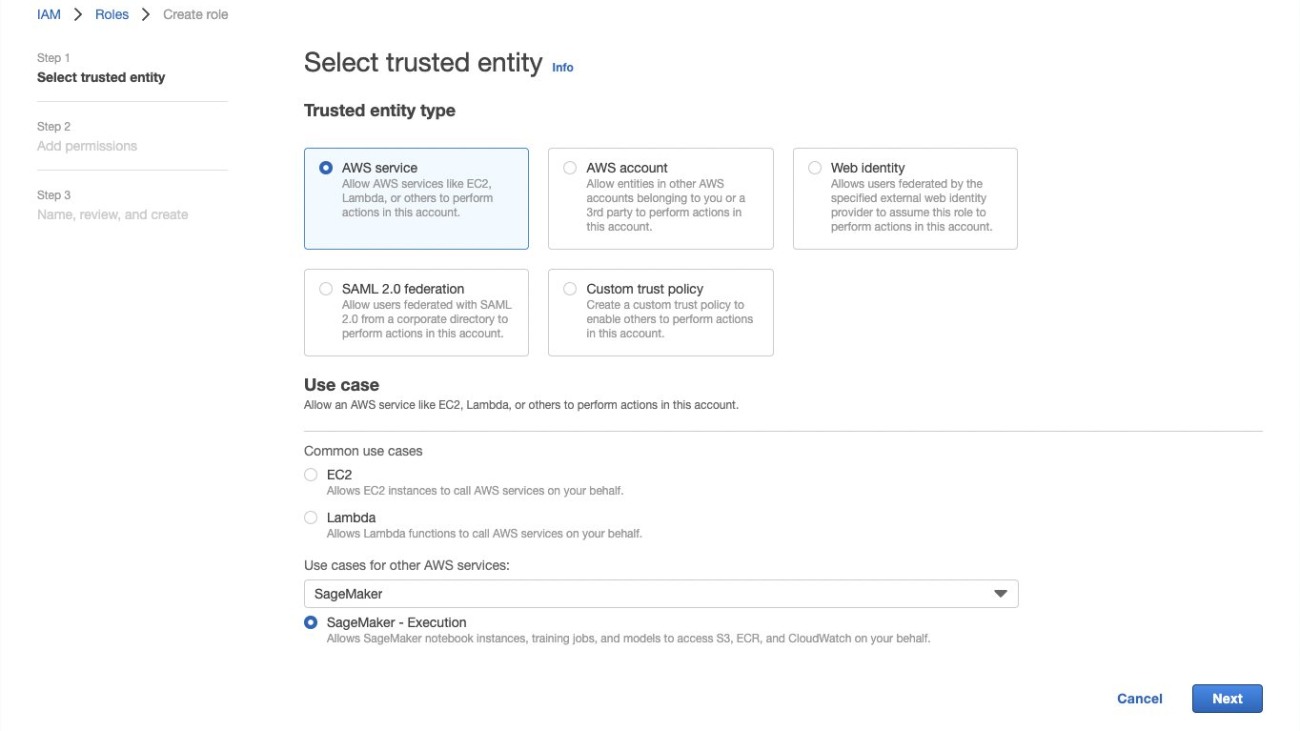
3. For Trusted entity type, select AWS service.
4. For Use cases for other AWS Services, choose SageMaker.
5. Select SageMaker – Execution.
6. Choose Next.
7. Review the permissions, then choose Next.
8. For Role name, enter a name (for this post, we use sagemaker-execution-role-notebook-jobs).
9. Choose Create role.
10. Make a note of the role ARN.

The role ARN will be in the format of arn:aws:iam::[account-number]:role/service-role/[role-name] and is required in the Studio Lab setup.

Create an IAM user

For a Studio Lab environment to access AWS, we need to create an IAM user within AWS and grant it necessary permissions. We then need to create a set of access keys for that user and provide them to the Studio Lab environment.

This step should be repeated for each SageMaker Studio Lab environment that will access this AWS account.

Note that administrators and AWS account owners should ensure that to the greatest extent possible, well-architected security practices are followed. For example, user permissions should always be scoped down, and access keys should be rotated regularly to minimize the impact of credential compromise.

In this blog we show how to use the AmazonSageMakerFullAccess managed policy. This policy provides broad access to Amazon SageMaker that may go beyond what is required. Details about AmazonSageMakerFullAccess can be found here.

Although Studio Lab employs enterprise security, it should be noted that Studio Lab user credentials don’t form part of your AWS account, and therefore, for example, are not subject to your AWS password or MFA policies.

To scope down permissions as much as possible, we create a user profile specifically for this access.

1. On the IAM console, choose Users in the navigation pane.
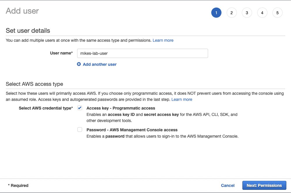
2. Choose Add users.
3. For User name, enter a name.It’s good practice to use a name that is linked to an individual person who will be using this account; this helps if reviewing audit logs.
4. For Select AWS access type, select Access key – Programmatic access.
5. Choose Next: Permissions.
6. Choose Attach existing policies directly.
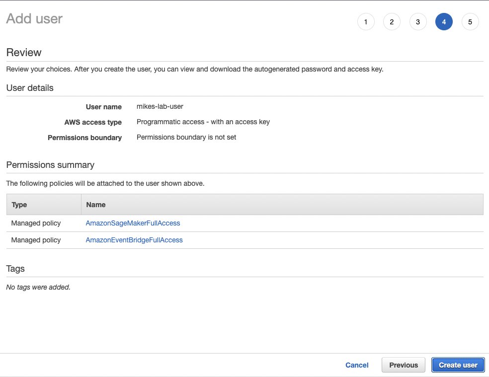
7. Search for and select AmazonSageMakerFullAccess.
8. Search for and select AmazonEventBridgeFullAccess.
9. Choose Next: Tags.
10. Choose Next: Review.
11. Confirm your policies, then choose Create user.The final page of the user creation process should show you the user’s access keys. Leave this tab open, because we can’t navigate back here and we need these details.
12. Open a new browser tab in Studio Lab.
13. On the File menu, choose New Launcher, then choose Terminal.
14. At the command line, enter the following code:

    aws configure

15. Enter the following code:
    1. Enter the values from the IAM console page for your access key ID and secret access key.
    2. For Default region name, enter us-west-2.
    3. Leave Default output format as text.

       (studiolab) studio-lab-user@default:~$ aws configure 
       AWS Access Key ID []: 01234567890
       AWS Secret Access Key []: ABCDEFG1234567890ABCDEFG
       Default region name []: us-west-2
       Default output format [text]: 
       
       (studiolab) studio-lab-user@default:~$

Congratulations, your Studio Lab environment should now be configured to access the AWS account. To test the connection, issue the following command:

aws sts get-caller-identity

This command should return details about the IAM user your configured to use.

Create a notebook job

Notebook jobs are created using Jupyter notebooks within Studio Lab. If your notebook runs in Studio Lab, then it can run as a notebook job (with more resources and access to AWS services). However, there are a couple of things to watch for.

If you have installed packages to get your notebook working, add commands to load these packages in a cell at the top of your notebook. By using a & symbol at the start of each line, the code will be sent to the command line to run. In the following example, the first cell uses pip to install PyTorch libraries:

%%capture
%pip install torch
%pip install torchvision

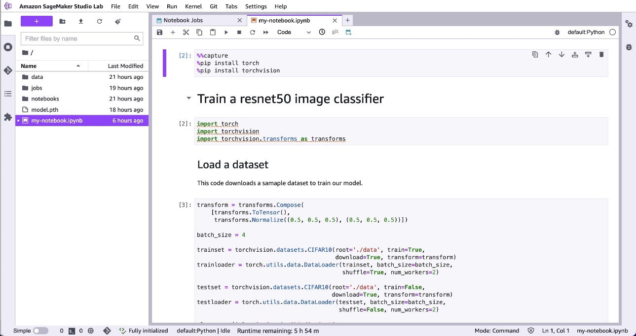
Our notebook will generate a trained PyTorch model. With our regular code, we save the model to the file system in Studio Labs.

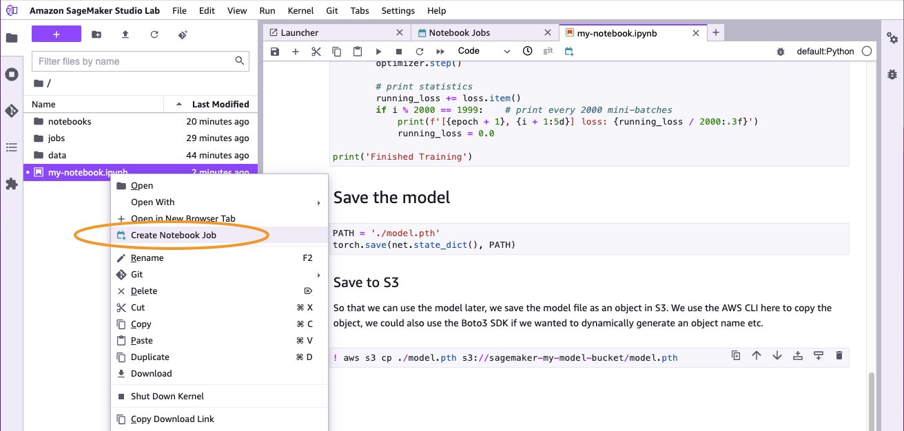
When we run this as a notebook job, we need to save the model somewhere we can access it afterwards. The easiest way to do this is to save the model in Amazon S3. We created an S3 bucket to save our models, and use another command line cell to copy the object into the bucket.

We use the AWS Command Line Interface (AWS CLI) here to copy the object. We could also use the AWS SDK for Python (Boto3) if we wanted to have a more sophisticated or automated control of the file name. For now, we will ensure that we change the file name each time we run the notebook so the models don’t get overwritten.

Now we are ready to create the notebook job.

1. Choose (right-click) the notebook name, then choose Create Notebook Job.
   If this menu option is missing, you may need to refresh your Studio Lab environment. To do this, open Terminal from the launcher and run the following code:

   conda deactivate && conda env remove —name studiolab

2. Next, restart your JupyterLab instance by choosing Amazon SageMaker Studio Lab from the top menu, then choose Restart JupyterLab.Alternatively, go to the project page, and shut down and restart the runtime.
3. On the Create job page, for Compute type, choose the compute type that suites your job.

   For more information on the different types of compute capacity, including the cost, see Amazon SageMaker Pricing (choose On-Demand Pricing and navigate to the Training tab. You may also need to check the quota availability of the compute type in your AWS account. For more information about service quotas, see: AWS service quotas.For this example, we’ve selected an ml.p3.2xlarge instance, which offers 8 vCPU, 61 GB of memory and a Tesla V100 GPU.

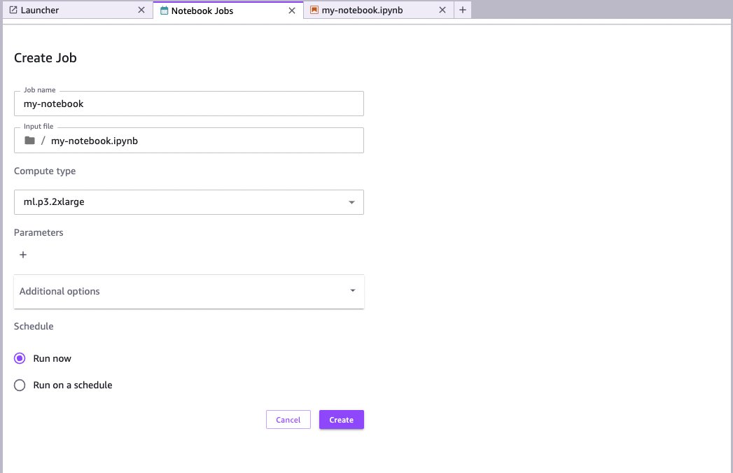
   If there are no warnings on this page, you should be ready to go. If there are warnings, check to ensure the correct role ARN is specified in Additional options. This role should match the ARN of the SageMaker execution role we created earlier.The ARN is in the format arn:aws:iam::[account-number]:role/service-role/[role-name].

   There are other options available within Additional options; for example, you can select a particular image and kernel that may already have the configuration you need without the need to install additional libraries.

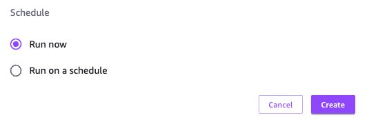
4. If you want to run this notebook on a schedule, select Run on a schedule and specify how often you want the job to run.We want this notebook to run once, so we select Run now.
5. Choose Create.
   

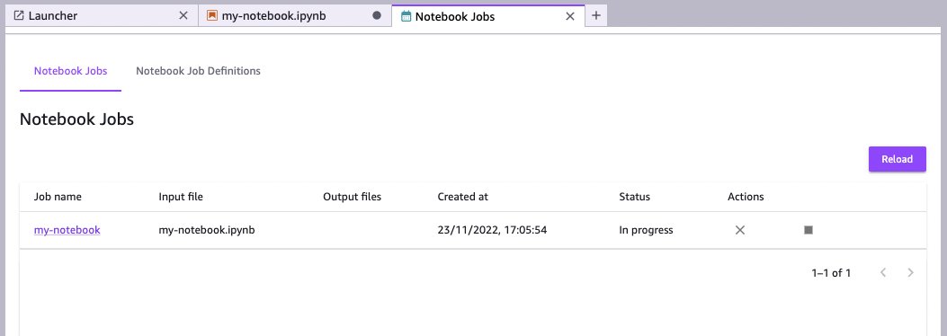
Notebook jobs list

The Notebook Jobs page lists all the jobs currently running and those that ran in the past. You can find this list from the Launcher (choose, File, New Launcher), then choose Notebook Jobs in the Other section.

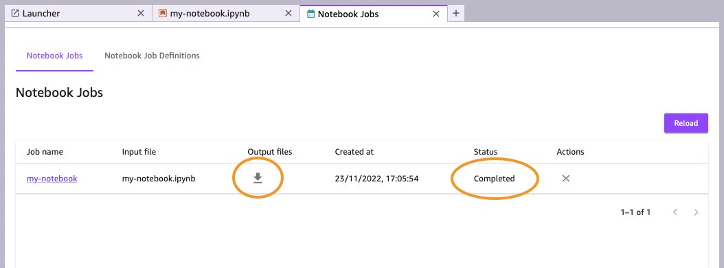
When the notebook job is complete, you will see the status change to Completed (use the Reload option if required). You can then choose the download icon to access the output files.

When the files have downloaded, you can review the notebook along with the code output and output log. In our case, because we added code to time the run of the training cell, we can see how long the training job took—16 minutes and 21 seconds, which is much faster than if the code had run inside of Studio Lab (1 hour, 38 minutes, 55 seconds). In fact, the whole notebook ran in 1,231 seconds (just over 20 minutes) at a cost of under $1.30 (USD).

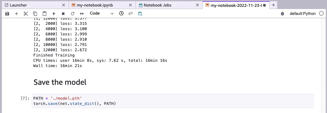
W can now increase the number of epochs and adjust the hyperparameters to improve the loss value of the model, and submit another notebook job.

Conclusion

In this post, we showed how to use Studio Lab notebook jobs to scale out the code we developed in Studio Lab and run it with more resources in an AWS account.

By adding AWS credentials to our Studio Lab environment, not only can we access notebook jobs, but we can also access other resources from an AWS account right from within our Studio Lab notebooks. Take a look at the AWS SDK for Python.

This extra capability of Studio Lab lifts the limits of the kinds and sizes of projects you can achieve. Let us know what you build with this new capability!

About the authors

Mike Chambers is a Developer Advocate for AI and ML at AWS. He has spent the last 7 years helping builders to learn cloud, security and ML. Originally from the UK, Mike is a passionate tea drinker and Lego builder.

Michele Monclova is a principal product manager at AWS on the SageMaker team. She is a native New Yorker and Silicon Valley veteran. She is passionate about innovations that improve our quality of life.

Read More