Learn about the development, operational, and process improvements that can be incorporated by organizations to improve the explainability of models while adhering to regulatory requirements.Read More
Introducing one-step classification and entity recognition with Amazon Comprehend for intelligent document processing
“Intelligent document processing (IDP) solutions extract data to support automation of high-volume, repetitive document processing tasks and for analysis and insight. IDP uses natural language technologies and computer vision to extract data from structured and unstructured content, especially from documents, to support automation and augmentation.” – Gartner
The goal of Amazon’s intelligent document processing (IDP) is to automate the processing of large amounts of documents using machine learning (ML) in order to increase productivity, reduce costs associated with human labor, and provide a seamless user experience. Customers spend a significant amount of time and effort identifying documents and extracting critical information from them for various use cases. Today, Amazon Comprehend supports classification for plain text documents, which requires you to preprocess documents in semi-structured formats (scanned, digital PDF or images such as PNG, JPG, TIFF) and then use the plain text output to run inference with your custom classification model. Similarly, for custom entity recognition in real time, preprocessing to extract text is required for semi-structured documents such as PDF and image files. This two-step process introduces complexities in document processing workflows.
Last year, we announced support for native document formats with custom named entity recognition (NER) asynchronous jobs. Today, we are excited to announce one-step document classification and real-time analysis for NER for semi-structured documents in native formats (PDF, TIFF, JPG, PNG) using Amazon Comprehend. Specifically, we are announcing the following capabilities:
- Support for documents in native formats for custom classification real-time analysis and asynchronous jobs
- Support for documents in native formats for custom entity recognition real-time analysis
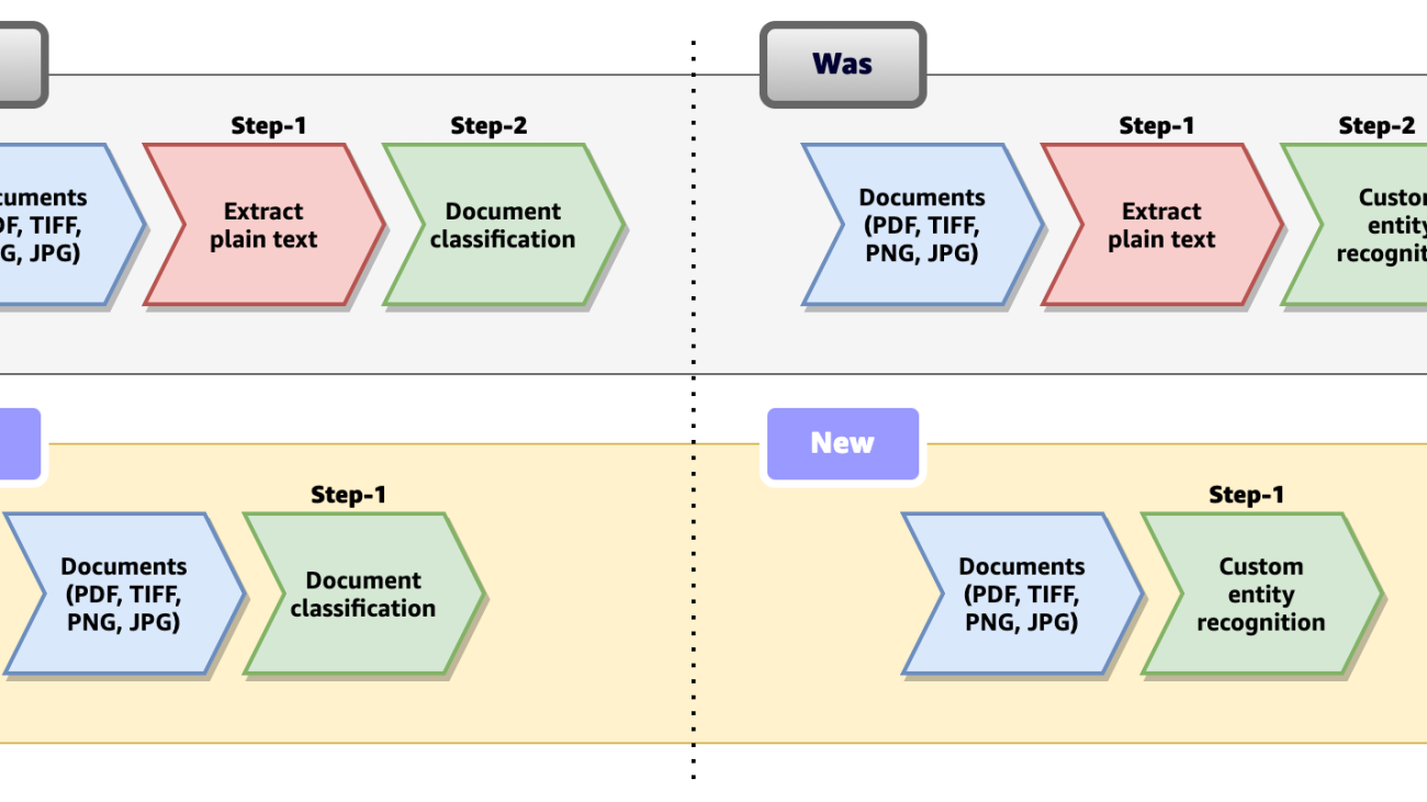
With this new release, Amazon Comprehend custom classification and custom entity recognition (NER) supports documents in formats such as PDF, TIFF, PNG, and JPEG directly, without the need to extract UTF8 encoded plain text from them. The following figure compares the previous process to the new procedure and support.
This feature simplifies document processing workflows by eliminating any preprocessing steps required to extract plain text from documents, and reduces the overall time required to process them.
In this post, we discuss a high-level IDP workflow solution design, a few industry use cases, the new features of Amazon Comprehend, and how to use them.
Overview of solution
Let’s start by exploring a common use case in the insurance industry. A typical insurance claim process involves a claim package that may contain multiple documents. When an insurance claim is filed, it includes documents like insurance claim form, incident reports, identity documents, and third-party claim documents. The volume of documents to process and adjudicate an insurance claim can run up to hundreds and even thousands of pages depending on the type of claim and business processes involved. Insurance claim representatives and adjudicators typically spend hundreds of hours manually sifting, sorting, and extracting information from hundreds or even thousands of claim filings.
Similar to the insurance industry use case, the payment industry also processes large volumes of semi-structured documents for cross-border payment agreements, invoices, and forex statements. Business users spend the majority of their time on manual activities such as identifying, organizing, validating, extracting, and passing required information to downstream applications. This manual process is tedious, repetitive, error prone, expensive, and difficult to scale. Other industries that face similar challenges include mortgage and lending, healthcare and life sciences, legal, accounting, and tax management. It is extremely important for businesses to process such large volumes of documents in a timely manner with a high level of accuracy and nominal manual effort.
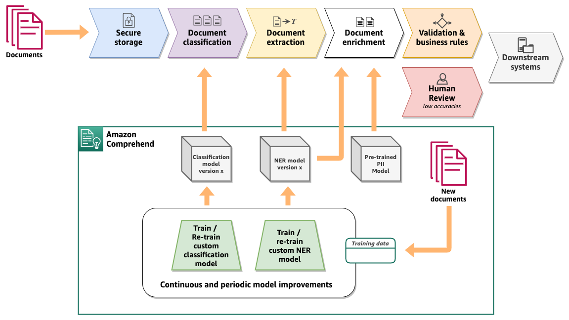
Amazon Comprehend provides key capabilities to automate document classification and information extraction from a large volume of documents with high accuracy, in a scalable and cost-effective way. The following diagram shows an IDP logical workflow with Amazon Comprehend. The core of the workflow consists of document classification and information extraction using NER with Amazon Comprehend custom models. The diagram also demonstrates how the custom models can be continuously improved to provide higher accuracies as documents and business processes evolve.
Custom document classification
With Amazon Comprehend custom classification, you can organize your documents into predefined categories (classes). At a high level, the following are the steps to set up a custom document classifier and perform document classification:
- Prepare training data to train a custom document classifier.
- Train a customer document classifier with the training data.
- After the model is trained, optionally deploy a real-time endpoint.
- Perform document classification with either an asynchronous job or in real time using the endpoint.
Steps 1 and 2 are typically done at the beginning of an IDP project after the document classes relevant to the business process are identified. A custom classifier model can then be periodically retrained to improve accuracy and introduce new document classes. You can train a custom classification model either in multi-class mode or multi-label mode. Training can be done for each in one of two ways: using a CSV file, or using an augmented manifest file. Refer to Preparing training data for more details on training a custom classification model. After a custom classifier model is trained, a document can be classified either using real-time analysis or an asynchronous job. Real-time analysis requires an endpoint to be deployed with the trained model and is best suited for small documents depending on the use case. For a large number of documents, an asynchronous classification job is best suited.
Train a custom document classification model
To demonstrate the new feature, we trained a custom classification model in multi-label mode, which can classify insurance documents into one of seven different classes. The classes are INSURANCE_ID, PASSPORT, LICENSE, INVOICE_RECEIPT, MEDICAL_TRANSCRIPTION, DISCHARGE_SUMMARY, and CMS1500. We want to classify sample documents in native PDF, PNG, and JPEG format, stored in an Amazon Simple Storage Service (Amazon S3) bucket, using the classification model. To start an asynchronous classification job, complete the following steps:
- On the Amazon Comprehend console, choose Analysis jobs in the navigation pane.
- Choose Create job.

- For Name, enter a name for your classification job.
- For Analysis type¸ choose Custom classification.
- For Classifier model, choose the appropriate trained classification model.
- For Version, choose the appropriate model version.

In the Input data section, we provide the location where our documents are stored.
- For Input format, choose One document per file.
- For Document read mode¸ choose Force document read action.
- For Document read action, choose Textract detect document text.
This enables Amazon Comprehend to use the Amazon Textract DetectDocumentText API to read the documents before running the classification. The DetectDocumentText API is helpful in extracting lines and words of text from the documents. You may also choose Textract analyze document for Document read action, in which case Amazon Comprehend uses the Amazon Textract AnalyzeDocument API to read the documents. With the AnalyzeDocument API, you can choose to extract Tables, Forms, or both. The Document read mode option enables Amazon Comprehend to extract the text from documents behind the scenes, which helps reduce the extra step of extracting text from the document, which is required in our document processing workflow.
The Amazon Comprehend custom classifier can also process raw JSON responses generated by the DetectDocumentText and AnalyzeDocument APIs, without any modification or preprocessing. This is useful for existing workflows where Amazon Textract is involved in extracting text from the documents already. In this case, the JSON output from Amazon Textract can be fed directly to the Amazon Comprehend document classification APIs.
- In the Output data section, for S3 location, specify an Amazon S3 location where you want the asynchronous job to write the results of the inference.
- Leave the remaining options as default.
- Choose Create job to start the job.

You can view the status of the job on the Analysis jobs page.
When the job is complete, we can view the output of the analysis job, which is stored in the Amazon S3 location provided during the job configuration. The classification output for our single-page PDF sample CMS1500 document is as follows. The output is a file in JSON lines format, which has been formatted to improve readability.
The preceding sample is a single-page PDF document; however, custom classification can also handle multi-page PDF documents. In the case of multi-page documents, the output contains multiple JSON lines, where each line is the classification result of each of the pages in a document. The following is a sample multi-page classification output:
Custom entity recognition
With an Amazon Comprehend custom entity recognizer, you can analyze documents and extract entities like product codes or business-specific entities that fit your particular needs. At a high level, the following are the steps to set up a custom entity recognizer and perform entity detection:
- Prepare training data to train a custom entity recognizer.
- Train a custom entity recognizer with the training data.
- After the model is trained, optionally deploy a real-time endpoint.
- Perform entity detection with either an asynchronous job or in real time using the endpoint.
A custom entity recognizer model can be periodically retrained to improve accuracy and to introduce new entity types. You can train a custom entity recognizer model with either entity lists or annotations. In both cases, Amazon Comprehend learns about the kind of documents and the context where the entities occur to build an entity recognizer model that can generalize to detect new entities. Refer to Preparing the training data to learn more about preparing training data for custom entity recognizer.
After a custom entity recognizer model is trained, entity detection can be done either using real-time analysis or an asynchronous job. Real-time analysis requires an endpoint to be deployed with the trained model and is best suited for small documents depending on the use case. For a large number of documents, an asynchronous classification job is best suited.
Train a custom entity recognition model
To demonstrate the entity detection in real time, we trained a custom entity recognizer model with insurance documents and augmented manifest files using custom annotations and deployed the endpoint using the trained model. The entity types are Law Firm, Law Office Address, Insurance Company, Insurance Company Address, Policy Holder Name, Beneficiary Name, Policy Number, Payout, Required Action, and Sender. We want to detect entities from sample documents in native PDF, PNG, and JPEG format, stored in an S3 bucket, using the recognizer model.
Note that you can use a custom entity recognition model that is trained with PDF documents to extract custom entities from PDF, TIFF, image, Word, and plain text documents. If your model is trained using text documents and an entity list, you can only use plain text documents to extract the entities.
We need to detect entities from a sample document in any native PDF, PNG, and JPEG format using the recognizer model. To start a synchronous entity detection job, complete the following steps:
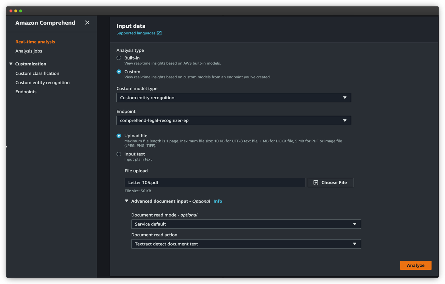
- On the Amazon Comprehend console, choose Real-time analysis in the navigation pane.
- Under Analysis type, select Custom.
- For Custom entity recognition, choose the custom model type.
- For Endpoint, choose the real-time endpoint that you created for your entity recognizer model.
- Select Upload file and choose Choose File to upload the PDF or image file for inference.
- Expand the Advanced document input section and for Document read mode, choose Service default.
- For Document read action, choose Textract detect document text.
- Choose Analyze to analyze the document in real time.
The recognized entities are listed in the Insights section. Each entity contains the entity value (the text), the type of entity as defined by your during the training process, and the corresponding confidence score.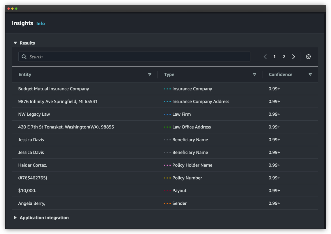
For more details and a complete walkthrough on how to train a custom entity recognizer model and use it to perform asynchronous inference using asynchronous analysis jobs, refer to Extract custom entities from documents in their native format with Amazon Comprehend.
Conclusion
This post demonstrated how you can classify and categorize semi-structured documents in their native format and detect business-specific entities from them using Amazon Comprehend. You can use real-time APIs for low-latency use cases, or use asynchronous analysis jobs for bulk document processing.
As a next step, we encourage you to visit the Amazon Comprehend GitHub repository for full code samples to try out these new features. You can also visit the Amazon Comprehend Developer Guide and Amazon Comprehend developer resources for videos, tutorials, blogs, and more.
About the authors
 Wrick Talukdar is a Senior Architect with the Amazon Comprehend Service team. He works with AWS customers to help them adopt machine learning on a large scale. Outside of work, he enjoys reading and photography.
 Anjan Biswas is a Senior AI Services Solutions Architect with a focus on AI/ML and Data Analytics. Anjan is part of the world-wide AI services team and works with customers to help them understand and develop solutions to business problems with AI and ML. Anjan has over 14 years of experience working with global supply chain, manufacturing, and retail organizations, and is actively helping customers get started and scale on AWS AI services.
 Godwin Sahayaraj Vincent is an Enterprise Solutions Architect at AWS who is passionate about machine learning and providing guidance to customers to design, deploy, and manage their AWS workloads and architectures. In his spare time, he loves to play cricket with his friends and tennis with his three kids.
Modeling Heart Rate Response to Exercise with Wearable Data
This paper was accepted at the workshop “Learning from Time Series for Health” at NeurIPS 2022.
Heart rate (HR) dynamics in response to workout intensity and duration measure key aspects of an individual’s fitness and cardiorespiratory health. Models of exercise physiology have been used to characterize cardiorespiratory fitness in well-controlled laboratory settings, but face additional challenges when applied to wearables in noisy, real-world settings. Here, we introduce a hybrid machine learning model that combines a physiological model of HR and demand during exercise with neural network…Apple Machine Learning Research
USC and Amazon select five new faculty research projects
Faculty projects are focused on various aspects of trustworthy machine learning.Read More

Speech AI Expands Global Reach With Telugu Language Breakthrough
More than 75 million people speak Telugu, predominantly in India’s southern regions, making it one of the most widely spoken languages in the country.
Despite such prevalence, Telugu is considered a low-resource language when it comes to speech AI. This means there aren’t enough hours’ worth of speech datasets to easily and accurately create AI models for automatic speech recognition (ASR) in Telugu.
And that means billions of people are left out of using ASR to improve transcription, translation and additional speech AI applications in Telugu and other low-resource languages.
To build an ASR model for Telugu, the NVIDIA speech AI team turned to the NVIDIA NeMo framework for developing and training state-of-the-art conversational AI models. The model won first place in a competition conducted in October by IIIT-Hyderabad, one of India’s most prestigious institutes for research and higher education.
NVIDIA placed first in accuracy for both tracks of the Telugu ASR Challenge, which was held in collaboration with the Technology Development for Indian Languages program and India’s Ministry of Electronics and Information Technology as a part of its National Language Translation Mission.
For the closed track, participants had to use around 2,000 hours of a Telugu-only training dataset provided by the competition organizers. And for the open track, participants could use any datasets and pretrained AI models to build the Telugu ASR model.
NVIDIA NeMo-powered models topped the leaderboards with a word error rate of approximately 13% and 12% for the closed and open tracks, respectively, outperforming by a large margin all models built on popular ASR frameworks like ESPnet, Kaldi, SpeechBrain and others.
“What sets NVIDIA NeMo apart is that we open source all of the models we have — so people can easily fine-tune the models and do transfer learning on them for their use cases,” said Nithin Koluguri, a senior research scientist on the conversational AI team at NVIDIA. “NeMo is also one of the only toolkits that supports scaling training to multi-GPU systems and multi-node clusters.”
Building the Telugu ASR Model
The first step in creating the award-winning model, Koluguri said, was to preprocess the data.
Koluguri and his colleague Megh Makwana, an applied deep learning solution architect manager at NVIDIA, removed invalid letters and punctuation marks from the speech dataset that was provided for the closed track of the competition.
“Our biggest challenge was dealing with the noisy data,” Koluguri said. “This is when the audio and the transcript don’t match — in this case you cannot guarantee the accuracy of the ground-truth transcript you’re training on.”
The team cleaned up the audio clips by cutting them to be less than 20 seconds, chopped out clips of less than 1 second and removed sentences with a greater-than-30 character rate, which measures characters spoken per second.
Makwana then used NeMo to train the ASR model for 160 epochs, or full cycles through the dataset, which had 120 million parameters.
For the competition’s open track, the team used models pretrained with 36,000 hours of data on all 40 languages spoken in India. Fine-tuning this model for the Telugu language took around three days using an NVIDIA DGX system, according to Makwana.
Inference test results were then shared with the competition organizers. NVIDIA won with around 2% better word error rates than the second-place participant. This is a huge margin for speech AI, according to Koluguri.
“The impact of ASR model development is very high, especially for low-resource languages,” he added. “If a company comes forward and sets a baseline model, as we did for this competition, people can build on top of it with the NeMo toolkit to make transcription, translation and other ASR applications more accessible for languages where speech AI is not yet prevalent.”
NVIDIA Expands Speech AI for Low-Resource Languages
“ASR is gaining a lot of momentum in India majorly because it will allow digital platforms to onboard and engage with billions of citizens through voice-assistance services,” Makwana said.
And the process for building the Telugu model, as outlined above, is a technique that can be replicated for any language.
Of around 7,000 world languages, 90% are considered to be low resource for speech AI — representing 3 billion speakers. This doesn’t include dialects, pidgins and accents.
Open sourcing all of its models on the NeMo toolkit is one way NVIDIA is improving linguistic inclusion in the field of speech AI.
In addition, pretrained models for speech AI, as part of the NVIDIA Riva software development kit, are now available in 10 languages — with many additions planned for the future.
And NVIDIA this month hosted its inaugural Speech AI Summit, featuring speakers from Google, Meta, Mozilla Common Voice and more. Learn more about “Unlocking Speech AI Technology for Global Language Users” by watching the presentation on demand.
Get started building and training state-of-the-art conversational AI models with NVIDIA NeMo.
The post Speech AI Expands Global Reach With Telugu Language Breakthrough appeared first on NVIDIA Blog.
Accelerating Hugging Face and TIMM models with PyTorch 2.0
torch.compile() makes it easy to experiment with different compiler backends to make PyTorch code faster with a single line decorator torch.compile(). It works either directly over an nn.Module as a drop-in replacement for torch.jit.script() but without requiring you to make any source code changes. We expect this one line code change to provide you with between 30%-2x training time speedups on the vast majority of models that you’re already running.
opt_module = torch.compile(module)
torch.compile supports arbitrary PyTorch code, control flow, mutation and comes with experimental support for dynamic shapes. We’re so excited about this development that we call it PyTorch 2.0.
What makes this announcement different for us is we’ve already benchmarked some of the most popular open source PyTorch models and gotten substantial speedups ranging from 30% to 2x https://github.com/pytorch/torchdynamo/issues/681.
There are no tricks here, we’ve pip installed popular libraries like https://github.com/huggingface/transformers, https://github.com/huggingface/accelerate and https://github.com/rwightman/pytorch-image-models and then ran torch.compile() on them and that’s it.
It’s rare to get both performance and convenience, but this is why the core team finds PyTorch 2.0 so exciting. The Hugging Face team is also excited, in their words:
Ross Wightman the primary maintainer of TIMM: “PT 2.0 works out of the box with majority of timm models for inference and train workloads and no code changes”
Sylvain Gugger the primary maintainer of transformers and accelerate: “With just one line of code to add, PyTorch 2.0 gives a speedup between 1.5x and 2.x in training Transformers models. This is the most exciting thing since mixed precision training was introduced!”
This tutorial will show you exactly how to replicate those speedups so you can be as excited as to PyTorch 2.0 as we are.
Requirements and Setup
For GPU (newer generation GPUs will see drastically better performance)
pip3 install numpy --pre torch[dynamo] --force-reinstall --extra-index-url https://download.pytorch.org/whl/nightly/cu117
For CPU
pip3 install --pre torch --extra-index-url https://download.pytorch.org/whl/nightly/cpu
Optional: Verify Installation
git clone https://github.com/pytorch/pytorch
cd tools/dynamo
python verify_dynamo.py
Optional: Docker installation
We also provide all the required dependencies in the PyTorch nightly
binaries which you can download with
docker pull ghcr.io/pytorch/pytorch-nightly
And for ad hoc experiments just make sure that your container has access
to all your GPUs
docker run --gpus all -it ghcr.io/pytorch/pytorch-nightly:latest /bin/bash
Getting started
a toy exmaple
Let’s start with a simple example and make things more complicated step
by step. Please note that you’re likely to see more significant speedups the newer your GPU is.
import torch
   def fn(x, y):
       a = torch.sin(x).cuda()
       b = torch.sin(y).cuda()
       return a + b
   new_fn = torch.compile("inductor")(fn)
   input_tensor = torch.randn(10000).to(device="cuda:0")
   a = new_fn()
This example won’t actually run faster but it’s a good educational.
example that features torch.cos() and torch.sin() which are examples of pointwise ops as in they operate element by element on a vector. A more famous pointwise op you might actually want to use would be something like torch.relu().
Pointwise ops in eager mode are suboptimal because each one would need to read a tensor from memory, make some changes and then write back those changes.
The single most important optimization that PyTorch 2.0 does for you is fusion.
So back to our example we can turn 2 reads and 2 writes into 1 read and 1 write which is crucial especially for newer GPUs where the bottleneck is memory bandwidth (how quickly you can send data to a GPU) instead of compute (how quickly your GPU can crunch floating point operations)
The second most important optimization that PyTorch 2.0 does for you is CUDA graphs
CUDA graphs help eliminate the overhead from launching individual kernels from a python program.
torch.compile() supports many different backends but one that we’re particularly excited about is Inductor which generates Triton kernels https://github.com/openai/triton which are written in Python yet outperform the vast majority of handwritten CUDA kernels. Suppose our example above was called trig.py we can actually inspect the code generated triton kernels by running.
TORCHINDUCTOR_TRACE=1 python trig.py
@pointwise(size_hints=[16384], filename=__file__, meta={'signature': {0: '*fp32', 1: '*fp32', 2: 'i32'}, 'device': 0, 'constants': {}, 'configs': [instance_descriptor(divisible_by_16=(0, 1, 2), equal_to_1=())]})
   @triton.jit
   def kernel(in_ptr0, out_ptr0, xnumel, XBLOCK : tl.constexpr):
       xnumel = 10000
       xoffset = tl.program_id(0) * XBLOCK
       xindex = xoffset + tl.reshape(tl.arange(0, XBLOCK), [XBLOCK])
       xmask = xindex < xnumel
       x0 = xindex
       tmp0 = tl.load(in_ptr0 + (x0), xmask)
       tmp1 = tl.sin(tmp0)
       tmp2 = tl.sin(tmp1)
       tl.store(out_ptr0 + (x0 + tl.zeros([XBLOCK], tl.int32)), tmp2, xmask)
And you can verify that fusing the two sins did actually occur because the two sin operations occur within a single Triton kernel and the temporary variables are held in registers with very fast access.
a real model
As a next step let’s try a real model like resnet50 from the PyTorch hub.
import torch
   model = torch.hub.load('pytorch/vision:v0.10.0', 'resnet18', pretrained=True)
   opt_model = torch.compile("inductor",model)
   model(torch.randn(1,3,64,64))
If you actually run you may be surprised that the first run is slow and that’s because the model is being compiled. Subsequent runs will be faster so it’s common practice to warm up your model before you start benchmarking it.
You may have noticed how we also passed in the name of a compiler explicitly here with “inductor” but it’s not the only available backend, you can run in a REPL torch._dynamo.list_backends() to see the full list of available backends. For fun you should try out aot_cudagraphs or nvfuser.
Hugging Face models
Let’s do something a bit more interesting now, our community frequently
uses pretrained models from transformers https://github.com/huggingface/transformers or TIMM https://github.com/rwightman/pytorch-image-models and one of our design goals for PyTorch 2.0 was that any new compiler stack needs to work out of the box with the vast majority of models people actually run.
So we’re going to directly download a pretrained model from the Hugging Face hub and optimize it
import torch
   from transformers import BertTokenizer, BertModel
   # Copy pasted from here https://huggingface.co/bert-base-uncased
   tokenizer = BertTokenizer.from_pretrained('bert-base-uncased')
   model = BertModel.from_pretrained("bert-base-uncased").to(device="cuda:0")
   model = torch.compile(model) # This is the only line of code that we changed
   text = "Replace me by any text you'd like."
   encoded_input = tokenizer(text, return_tensors='pt').to(device="cuda:0")
   output = model(**encoded_input)
If you remove the to(device="cuda:0") from the model and encoded_input then PyTorch 2.0 will generate C++ kernels that will be optimized for running on your CPU. You can inspect both Triton or C++ kernels for BERT, they’re obviously more complex than the trigonometry example we had above but you can similarly skim it and understand if you understand PyTorch.
The same code also works just fine if used with https://github.com/huggingface/accelerate and DDP
Similarly let’s try out a TIMM example
import timm
   import torch
   model = timm.create_model('resnext101_32x8d', pretrained=True, num_classes=2)
   opt_model = torch.compile(model, "inductor")
   opt_model(torch.randn(64,3,7,7))
Our goal with PyTorch was to build a breadth-first compiler that would speed up the vast majority of actual models people run in open source. The Hugging Face Hub ended up being an extremely valuable benchmarking tool for us, ensuring that any optimization we work on actually helps accelerate models people want to run.
So please try out PyTorch 2.0, enjoy the free perf and if you’re not seeing it then please open an issue and we will make sure your model is supported https://github.com/pytorch/torchdynamo/issues
After all, we can’t claim we’re created a breadth-first unless YOUR models actually run faster.
Get Started with PyTorch 2.0 Summary and Overview
Introducing PyTorch 2.0, our first steps toward the next generation 2-series release of PyTorch. Over the last few years we have innovated and iterated from PyTorch 1.0 to the most recent 1.13 and moved to the newly formed PyTorch Foundation, part of the Linux Foundation.
To complement the PyTorch 2.0 announcement and conference, we have also posted a comprehensive introduction and technical overview within the Get Started menu at https://pytorch.org/get-started/pytorch-2.0.
We also wanted to ensure you had all the information to quickly leverage PyTorch 2.0 in your models so we added the technical requirements, tutorial, user experience, Hugging Face benchmarks and FAQs to get you started today!
Finally we are launching a new “Ask the Engineers: 2.0 Live Q&A” series that allows you to go deeper on a range of topics with PyTorch subject matter experts. We hope this content is helpful for the entire community and level of users/contributors.
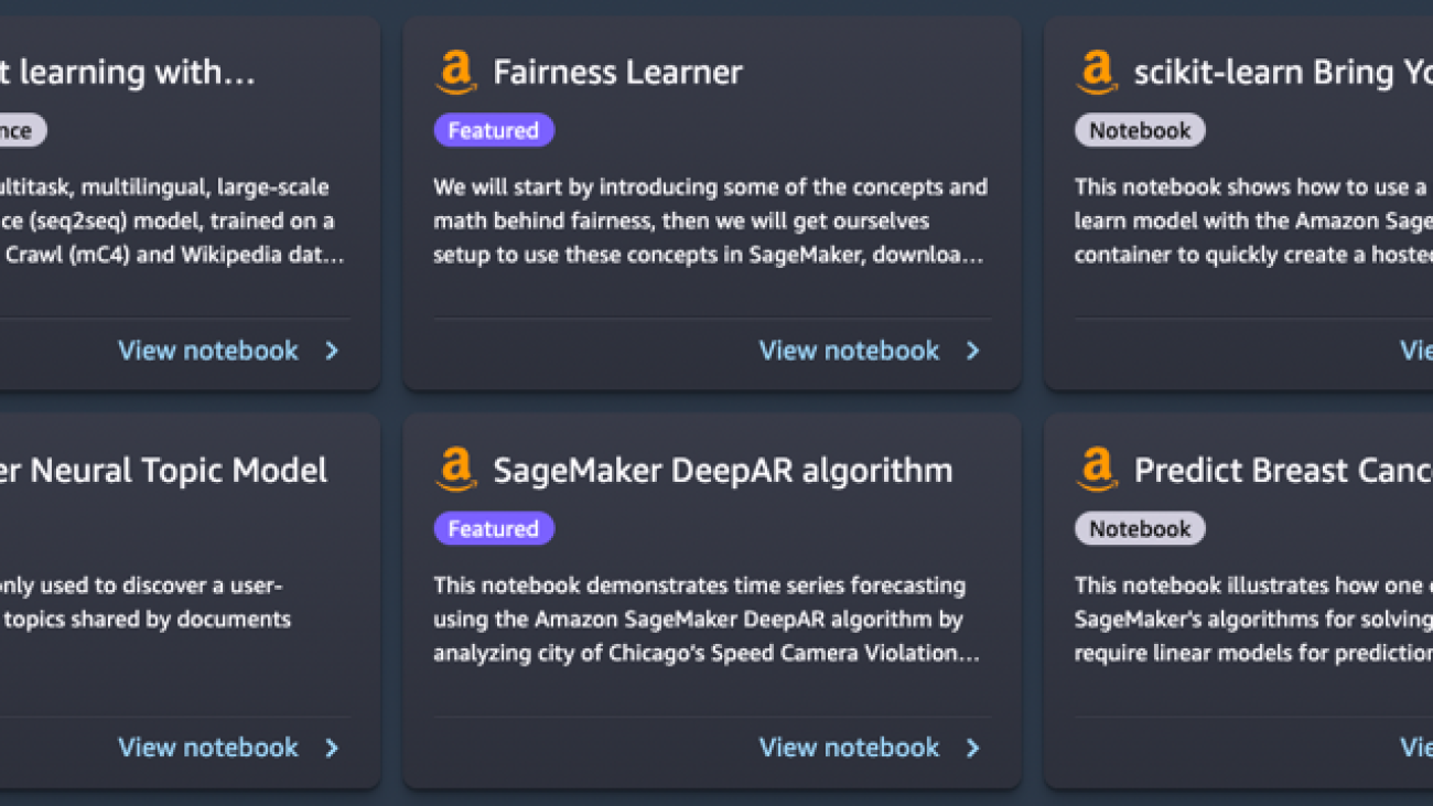
Illustrative notebooks in Amazon SageMaker JumpStart
Amazon SageMaker JumpStart is the Machine Learning (ML) hub of SageMaker providing pre-trained, publicly available models for a wide range of problem types to help you get started with machine learning.
JumpStart also offers example notebooks that use Amazon SageMaker features like spot instance training and experiments over a large variety of model types and use cases. These example notebooks contain code that shows how to apply ML solutions by using SageMaker and JumpStart. They can be adapted to match to your own needs and can thus speed up application development.
Recently, we added 10 new notebooks to JumpStart in Amazon SageMaker Studio. This post focuses on these new notebooks. As of this writing, JumpStart offers 56 notebooks, ranging from using state-of-the-art natural language processing (NLP) models to fixing bias in datasets when training models.
The 10 new notebooks can help you in the following ways:
- They offer example code for you to run as is from the JumpStart UI in Studio and see how the code works
- They show the usage of various SageMaker and JumpStart APIs
- They offer a technical solution that you can further customize based on your own needs
The number of notebooks that are offered through JumpStart increase on a regular basis as more notebooks are added. These notebooks are also available on github.

Notebooks overview
The 10 new notebooks are as follows:
- In-context learning with AlexaTM 20B – Demonstrates how to use AlexaTM 20B for in-context learning with zero-shot and few-shot learning on five example tasks: text summarization, natural language generation, machine translation, extractive question answering, and natural language inference and classification.
- Fairness linear learner in SageMaker – There have recently been concerns about bias in ML algorithms as a result of mimicking existing human prejudices. This notebook applies fairness concepts to adjust model predictions appropriately.
- Manage ML experimentation using SageMaker Search – Amazon SageMaker Search lets you quickly find and evaluate the most relevant model training runs from potentially hundreds and thousands of SageMaker model training jobs.
- SageMaker Neural Topic Model – SageMaker Neural Topic Model (NTM) is an unsupervised learning algorithm that attempts to describe a set of observations as a mixture of distinct categories.
- Predict driving speed violations – The SageMaker DeepAR algorithm can be used to train a model for multiple streets simultaneously, and predict violations for multiple street cameras.
- Breast cancer prediction – This notebook uses UCI’S breast cancer diagnostic dataset to build a predictive model of whether a breast mass image indicates a benign or malignant tumor.
- Ensemble predictions from multiple models – By combining or averaging predictions from multiple sources and models, we typically get an improved forecast. This notebook illustrates this concept.
- SageMaker asynchronous inference – Asynchronous inference is a new inference option for near-real-time inference needs. Requests can take up to 15 minutes to process and have payload sizes of up to 1 GB.
- TensorFlow bring your own model – Learn how to train a TensorFlow model locally and deploy on SageMaker using this notebook.
- Scikit-learn bring your own model – This notebook shows how to use a pre-trained Scikit-learn model with the SageMaker Scikit-learn container to quickly create a hosted endpoint for that model.
Prerequisites
To use these notebooks, make sure that you have access to Studio with an execution role that allows you to run SageMaker functionality. The short video below will help you navigate to JumpStart notebooks.
In the following sections, we go through each of the 10 new solutions and discuss some of their interesting details.
In-context learning with AlexaTM 20B
AlexaTM 20B is a multitask, multilingual, large-scale sequence-to-sequence (seq2seq) model, trained on a mixture of Common Crawl (mC4) and Wikipedia data across 12 languages, using denoising and Causal Language Modeling (CLM) tasks. It achieves state-of-the-art performance on common in-context language tasks such as one-shot summarization and one-shot machine translation, outperforming decoder only models such as Open AI’s GPT3 and Google’s PaLM, which are over eight times bigger.
In-context learning, also known as prompting, refers to a method where you use an NLP model on a new task without having to fine-tune it. A few task examples are provided to the model only as part of the inference input, a paradigm known as few-shot in-context learning. In some cases, the model can perform well without any training data at all, only given an explanation of what should be predicted. This is called zero-shot in-context learning.
This notebook demonstrates how to deploy AlexaTM 20B through the JumpStart API and run inference. It also demonstrates how AlexaTM 20B can be used for in-context learning with five example tasks: text summarization, natural language generation, machine translation, extractive question answering, and natural language inference and classification.
 |
 |
The notebook demonstrates the following:
- One-shot text summarization, natural language generation, and machine translation using a single training example for each of these tasks
- Zero-shot question answering and natural language inference plus classification using the model as is, without the need to provide any training examples.
Try running your own text against this model and see how it summarizes text, extracts Q&A, or translates from one language to another.
Fairness linear learner in SageMaker
There have recently been concerns about bias in ML algorithms as a result of mimicking existing human prejudices. Nowadays, several ML methods have strong social implications, for example they are used to predict bank loans, insurance rates, or advertising. Unfortunately, an algorithm that learns from historical data will naturally inherit past biases. This notebook presents how to overcome this problem by using SageMaker and fair algorithms in the context of linear learners.
It starts by introducing some of the concepts and math behind fairness, then it downloads data, trains a model, and finally applies fairness concepts to adjust model predictions appropriately.
 |
 |
The notebook demonstrates the following:
- Running a standard linear model on UCI’s Adult dataset.
- Showing unfairness in model predictions
- Fixing data to remove bias
- Retraining the model
Try running your own data using this example code and detect if there is bias. After that, try removing bias, if any, in your dataset using the provided functions in this example notebook.
Manage ML experimentation using SageMaker Search
SageMaker Search lets you quickly find and evaluate the most relevant model training runs from potentially hundreds and thousands of SageMaker model training jobs. Developing an ML model requires continuous experimentation, trying new learning algorithms, and tuning hyperparameters, all while observing the impact of such changes on model performance and accuracy. This iterative exercise often leads to an explosion of hundreds of model training experiments and model versions, slowing down the convergence and discovery of a winning model. In addition, the information explosion makes it very hard down the line to trace back the lineage of a model version—the unique combination of datasets, algorithms, and parameters that brewed that model in the first place.
This notebook shows how to use SageMaker Search to quickly and easily organize, track, and evaluate your model training jobs on SageMaker. You can search on all the defining attributes from the learning algorithm used, hyperparameter settings, training datasets used, and even the tags you have added on the model training jobs. You can also quickly compare and rank your training runs based on their performance metrics, such as training loss and validation accuracy, thereby creating leaderboards for identifying the winning models that can be deployed into production environments. SageMaker Search can quickly trace back the complete lineage of a model version deployed in a live environment, right up until the datasets used in training and validating the model.
 |
 |
The notebook demonstrates the following:
- Training a linear model three times
- Using SageMaker Search to organize and evaluate these experiments
- Visualizing the results in a leaderboard
- Deploying a model to an endpoint
- Tracing lineage of the model starting from the endpoint
In your own development of predictive models, you may be running several experiments. Try using SageMaker Search in such experiments and experience how it can help you in multiple ways.
SageMaker Neural Topic Model
SageMaker Neural Topic Model (NTM) is an unsupervised learning algorithm that attempts to describe a set of observations as a mixture of distinct categories. NTM is most commonly used to discover a user-specified number of topics shared by documents within a text corpus. Here each observation is a document, the features are the presence (or occurrence count) of each word, and the categories are the topics. Because the method is unsupervised, the topics aren’t specified up-front and aren’t guaranteed to align with how a human may naturally categorize documents. The topics are learned as a probability distribution over the words that occur in each document. Each document, in turn, is described as a mixture of topics.
This notebook uses the SageMaker NTM algorithm to train a model on the 20NewsGroups dataset. This dataset has been widely used as a topic modeling benchmark.
 |
 |
The notebook demonstrates the following:
- Creating a SageMaker training job on a dataset to produce an NTM model
- Using the model to perform inference with a SageMaker endpoint
- Exploring the trained model and visualizing learned topics
You can easily modify this notebook to run on your text documents and divide them into various topics.
Predict driving speed violations
This notebook demonstrates time series forecasting using the SageMaker DeepAR algorithm by analyzing the city of Chicago’s Speed Camera Violation dataset. The dataset is hosted by Data.gov, and is managed by the U.S. General Services Administration, Technology Transformation Service.
These violations are captured by camera systems and are available to improve the lives of the public through the city of Chicago data portal. The Speed Camera Violation dataset can be used to discern patterns in the data and gain meaningful insights.
The dataset contains multiple camera locations and daily violation counts. Each daily violation count for a camera can be considered a separate time series. You can use the SageMaker DeepAR algorithm to train a model for multiple streets simultaneously, and predict violations for multiple street cameras.
 |
 |
The notebook demonstrates the following:
- Training the SageMaker DeepAR algorithm on the time series dataset using spot instances
- Making inferences on the trained model to make traffic violation predictions
With this notebook, you can learn how time series problems can be solved using the DeepAR algorithm in SageMaker and try applying it on your own time series datasets.
Breast cancer prediction
This notebook takes an example for breast cancer prediction using UCI’S breast cancer diagnostic dataset. It uses this dataset to build a predictive model of whether a breast mass image indicates a benign or malignant tumor.
 |
 |
The notebook demonstrates the following:
- Basic setup for using SageMaker
- Converting datasets to Protobuf format used by the SageMaker algorithms and uploading to Amazon Simple Storage Service (Amazon S3)
- Training a SageMaker linear learner model on the dataset
- Hosting the trained model
- Scoring using the trained model
You can go through this notebook to learn how to solve a business problem using SageMaker, and understand the steps involved for training and hosting a model.
Ensemble predictions from multiple models
In practical applications of ML on predictive tasks, one model often doesn’t suffice. Most prediction competitions typically require combining forecasts from multiple sources to get an improved forecast. By combining or averaging predictions from multiple sources or models, we typically get an improved forecast. This happens because there is considerable uncertainty in the choice of the model and there is no one true model in many practical applications. Therefore, it’s beneficial to combine predictions from different models. In the Bayesian literature, this idea is referred to as Bayesian model averaging, and has been shown to work much better than just picking one model.
This notebook presents an illustrative example to predict if a person makes over $50,000 a year based on information about their education, work experience, gender, and more.
 |
 |
The notebook demonstrates the following:
- Preparing your SageMaker notebook
- Loading a dataset from Amazon S3 using SageMaker
- Investigating and transforming the data so that it can be fed to SageMaker algorithms
- Estimating a model using the SageMaker XGBoost (Extreme Gradient Boosting) algorithm
- Hosting the model on SageMaker to make ongoing predictions
- Estimating a second model using the SageMaker linear learner method
- Combining the predictions from both models and evaluating the combined prediction
- Generating final predictions on the test dataset
Try running this notebook on your dataset and using multiple algorithms. Try experimenting with various combination of models offered by SageMaker and JumpStart and see which combination of model ensembling gives the best results on your own data.
SageMaker asynchronous inference
SageMaker asynchronous inference is a new capability in SageMaker that queues incoming requests and processes them asynchronously. SageMaker currently offers two inference options for customers to deploy ML models: a real-time option for low-latency workloads, and batch transform, an offline option to process inference requests on batches of data available up-front. Real-time inference is suited for workloads with payload sizes of less than 6 MB and require inference requests to be processed within 60 seconds. Batch transform is suitable for offline inference on batches of data.
Asynchronous inference is a new inference option for near-real-time inference needs. Requests can take up to 15 minutes to process and have payload sizes of up to 1 GB. Asynchronous inference is suitable for workloads that don’t have subsecond latency requirements and have relaxed latency requirements. For example, you might need to process an inference on a large image of several MBs within 5 minutes. In addition, asynchronous inference endpoints let you control costs by scaling down endpoint instance count to zero when they’re idle, so you only pay when your endpoints are processing requests.
 |
 |
The notebook demonstrates the following:
- Creating a SageMaker model
- Creating an endpoint using this model and asynchronous inference configuration
- Making predictions against this asynchronous endpoint
This notebook shows you a working example of putting together an asynchronous endpoint for a SageMaker model.
TensorFlow bring your own model
A TensorFlow model is trained locally on a classification task where this notebook is being run. Then it’s deployed on a SageMaker endpoint.
 |
 |
The notebook demonstrates the following:
- Training a TensorFlow model locally on the IRIS dataset
- Importing that model into SageMaker
- Hosting it on an endpoint
If you have TensorFlow models that you developed yourself, this example notebook can help you host your model on a SageMaker managed endpoint.
Scikit-learn bring your own model
SageMaker includes functionality to support a hosted notebook environment, distributed, serverless training, and real-time hosting. It works best when all three of these services are used together, but they can also be used independently. Some use cases may only require hosting. Maybe the model was trained prior to SageMaker existing, in a different service.

The notebook demonstrates the following:
- Using a pre-trained Scikit-learn model with the SageMaker Scikit-learn container to quickly create a hosted endpoint for that model
If you have Scikit-learn models that you developed yourself, this example notebook can help you host your model on a SageMaker managed endpoint.
Clean up resources
After you’re done running a notebook in JumpStart, make sure to Delete all resources so that all the resources that you created in the process are deleted and your billing is stopped. The last cell in these notebooks usually deletes endpoints that are created.
Summary
This post walked you through 10 new example notebooks that were recently added to JumpStart. Although this post focused on these 10 new notebooks, there are a total of 56 available notebooks as of this writing. We encourage you to log in to Studio and explore the JumpStart notebooks yourselves, and start deriving immediate value out of them. For more information, refer to Amazon SageMaker Studio and SageMaker JumpStart.
About the Author
 Dr. Raju Penmatcha is an AI/ML Specialist Solutions Architect in AI Platforms at AWS. He received his PhD from Stanford University. He works closely on the low/no-code suite services in SageMaker that help customers easily build and deploy machine learning models and solutions.
AWS CodeWhisperer creates computer code from natural language
At re:Invent, AWS announces that the CodeWhisperer preview has added support for two new programming languages.Read More
AWS CodeWhisperer creates computer code from natural language
At re:Invent, AWS announces that the CodeWhisperer preview has added support for two new programming languages.Read More