Meta set a goal to reach net zero emissions by 2030. We are developing technology to mitigate our carbon footprint and making these openly available.Read More

Experience the power of PyTorch 2.0 on AMD Solutions
PyTorch 2.0 represents a significant step forward for the PyTorch machine learning framework. The stable release of PyTorch 2.0 brings new features that unlock even higher performance, while remaining backward compatible with prior releases and retaining the Pythonic focus which has helped to make PyTorch so enthusiastically adopted by the AI/ML community. AMD has long been a strong proponent of PyTorch, and we are delighted that the PyTorch 2.0 stable release includes support for AMD Instinct™ and Radeon™ GPUs that are supported by the ROCm™ software platform.
With the stable PyTorch 2.0 release, PyTorch 2.0 introduces torch.compile as a beta feature underpinned by TorchInductor with support for AMD Instinct and Radeon GPUs through OpenAI Triton deep learning compiler. Through TorchInductor, developers can now generate low level kernels using Triton that are portable and performant to hand-written kernels on native hardware centric kernel programming models.
OpenAI Triton is a language and compiler for blocked algorithms, which aims to provide an abstraction layer between CUDA/HIP and Torch at which developers can write efficient kernels more productively. We have written a new backend which interfaces Triton’s custom MLIR dialects with our ROCm compiler stack.
Triton can automatically optimize kernels generated by machine learning compilers such as TorchInductor for multiple AI accelerators including AMD Instinct GPU accelerator by leveraging hardware-specific features of the AMD CDNA™ GPU architecture. This makes it easy for developers and users to switch seamlessly from any HW to AMD Instinct GPU accelerators and get great out of the box performance.
In addition, compilers like Triton can also enable developers to use high-level programming languages, such as Python, to write machine learning code that can be efficiently compiled and executed on specialized hardware. This can help greatly improve the productivity of machine learning developers, as they can focus on the algorithmic aspects of their models and rely on the compiler to generate efficient code.
By design, PyTorch 2.0 is backward compatible to earlier PyTorch releases. This holds true for the ROCm build of PyTorch 2.0 as well. Developers using PyTorch with AMD GPUs can migrate to PyTorch 2.0 with the confidence that their existing code will continue to work without any required changes, so there is no penalty to access the improvements that come with this release. On the other hand, using PyTorch 2.0 and TorchInductor can result in significant performance improvement over the default eager-mode as shown below.
The initial results using AMD Instinct MI250 GPUs already shows strong performance improvement with minimal optimization on TorchInductor compared to the default eager-mode. We see an average performance increase of up to 1.54X on 44 out of the 45 models on HuggingFace benchmarks suite with CamemBert, DistillGPT2 and T5Small being a few of the standout models with up to 1.5X or more performance improvement over eager-mode. We are looking forward to continued engagement with members of the PyTorch team at Meta to enable further optimization on ROCm software stack and the additional performance improvement for future PyTorch releases.
Image 1: AMD MI250 GPU performance improvement for TorchInductor vs eager-mode using HuggingFace MI200-89.
PyTorch 2.0 follows the same set of install options as before to build and install for supporting AMD GPUs. These include an installable Python package hosted at pytorch.org, AMD’s public PyTorch docker image, and of course the option to build from source using the upstream PyTorch repository. As with PyTorch builds for other platforms, the specific command line to be run for pip-based install is provided by the configurator at https://pytorch.org/get-started/locally/.
The GPUs supported by the ROCm software platform which forms the basis for PyTorch support on AMD GPUs are documented at https://docs.amd.com/bundle/Hardware_and_Software_Reference_Guide/page/Hardware_and_Software_Support.html
Conclusion
PyTorch 2.0 represents a major step in continuing to broaden support for ML developers by increasing performance while maintaining a simple, Pythonic interface. This performance uplift is made possible in large part by the new TorchInductor infrastructure, which in turn harnesses the Triton ML programming language and just-in-time compiler. AMD’s support for these technologies allows users to realize the full promise of the new PyTorch architecture. Our GPU support in PyTorch 2.0 is just one manifestation of a larger vision around AI and machine learning. AI/ML plays an important role in multiple AMD product lines, including Instinct and Radeon GPUs, Alveo™ data center accelerators, and both Ryzen™ and EPYC processors. These hardware and software initiatives are all part of AMD’s Pervasive AI vision, and we look forward to addressing the many new challenges and opportunities of this dynamic space.
MI200-89 – PyTorch Inductor mode HuggingFace Transformers training speedup, running the standard PyTorch 2.0 test suite, over PyTorch eager-mode comparison based on AMD internal testing on a single GCD as of 3/10/2023 using a 2P AMD EPYC™ 7763 production server with 4x AMD Instinct™ MI250 (128GB HBM2e) 560W GPUs with Infinity Fabric™ technology; host ROCm™ 5.3, guest ROCm™ 5.4.4, PyTorch 2.0.0, Triton 2.0. Server manufacturers may vary configurations, yielding different results. Performance may vary based on factors including use of latest drivers and optimizations.
© 2023 Advanced Micro Devices, Inc. All rights reserved. AMD, the AMD Arrow logo, AMD CDNA, AMD Instinct, EPYC, Radeon, ROCm, Ryzen, and combinations thereof are trademarks of Advanced Micro Devices, Inc. Other product names used in this publication are for identification purposes only and may be trademarks of their respective owners.
TIDEE: An Embodied Agent that Tidies Up Novel Rooms using Commonsense Priors
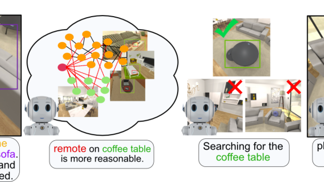
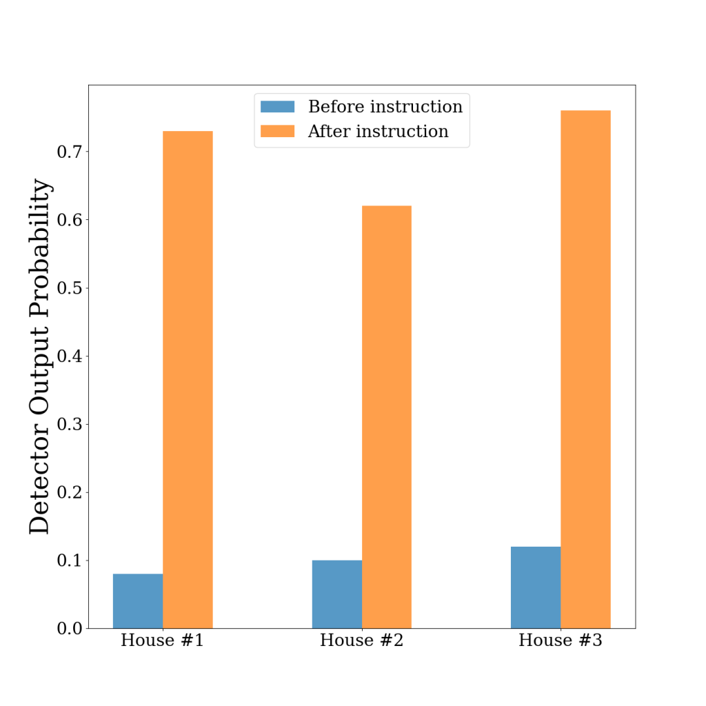
Example of embodied commonsense reasoning. A robot proactively identifies a remote on the floor and knows it is out of place without instruction. Then, the robot figures out where to place it in the scene and manipulates it there.
For robots to operate effectively in the world, they should be more than explicit step-by-step instruction followers. Robots should take actions in situations when there is a clear violation of the normal circumstances and be able to infer relevant context from partial instruction. Consider a situation where a home robot identifies a remote control which has fallen to the kitchen floor. The robot should not need to wait until a human instructs the robot to “pick the remote control off the floor and place it on the coffee table”. Instead, the robot should understand that the remote on the floor is clearly out of place, and act to pick it up and place it in a reasonable location. Even if a human were to spot the remote control first and instruct the agent to “put away the remote that is on the living room floor”, the robot should not require a second instruction for where to put the remote, but instead infer from experience that a reasonable location would be, for example, on the coffee table. After all, it would become tiring for a home robot user to have to specify every desire in excruciating detail (think about for each item you want the robot to move, specifying an instruction such as “pick up the shoes beneath the coffee table and place them next to the door, aligned with the wall”).
The type of reasoning that would permit such partial or self-generated instruction following involves a deep sense of how things in the world (objects, physics, other agents, etc.) ought to behave. Reasoning and acting of this kind are all aspects of embodied commonsense reasoning and are vastly important for robots to act and interact seamlessly in the physical world.
There has been much work on embodied agents that follow detailed step-by-step instructions, but less on embodied commonsense reasoning, where the task involves learning how to perceive and act without explicit instruction. One task in which to study embodied commonsense reasoning is that of tidying up, where the agent must identify objects which are out of their natural locations and act in order bring the identified objects to plausible locations. This task combines many desirable capabilities of intelligent agents with commonsense reasoning of object placements. The agent must search in likely locations for objects to be displaced, identify when objects are out of their natural locations in the context of the current scene, and figure out where to reposition the objects so that they are in proper locations – all while intelligently navigating and manipulating.
In our recent work, we propose TIDEE, an embodied agent that can tidy up never-before-seen rooms without any explicit instruction. TIDEE is the first of its kind for its ability to search a scene for out of place objects, identify where in the scene to reposition the out of place objects, and effectively manipulate the objects to the identified locations. We’ll walk through how TIDEE is able to do this in a later section, but first let’s describe how we create a dataset to train and test our agent for the task of tidying up.
Creating messy homes
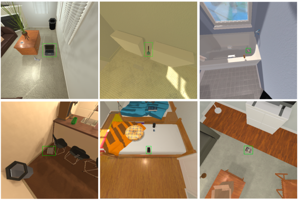
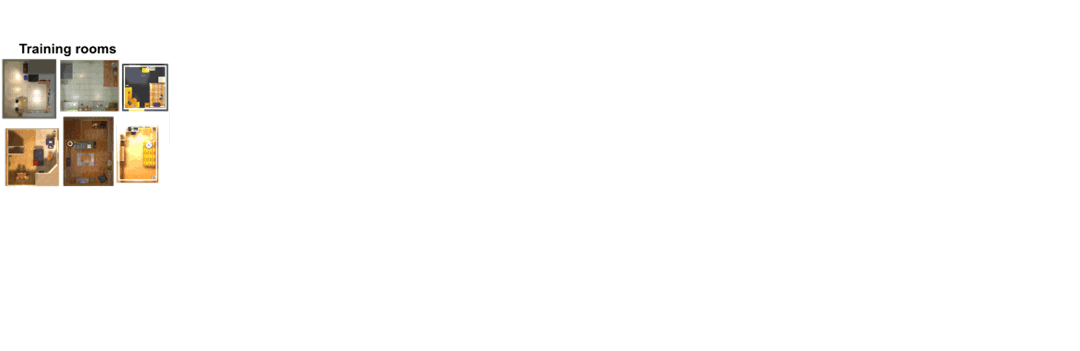
To create clean and messy scenes for our agent to learn from for what constitutes a tidy scene and what constitute a messy scene, we use a simulation environment called ai2thor. Ai2thor is an interactive 3D environment of indoor scenes that allows objects to be picked up and moved around. The simulator comes ready with 120 scenes of kitchens, bathrooms, living rooms, and bedrooms with over 116 object categories (and significantly more object instances) scattered throughout. Each of the scenes comes with a default initialization of object placements that are meticulously chosen by humans to be highly structured and “neat”. These default object locations make up our “tidy” scenes for providing our agent examples of objects in their natural locations. To create messy scenes, we apply forces to a subset of the objects with a random direction and magnitude (we “throw” the objects around) so they end up in uncommon locations and poses. You can see below some examples of objects which have been moved out of place.
Next, let’s see how TIDEE learns from this dataset to be able to tidy up rooms.
How does TIDEE work?
We give our agent a depth and RGB sensor to use for perceiving the scene. From this input, the agent must navigate around, detect objects, pick them up, and place them. The goal of the tidying task is to rearrange a messy room back to a tidy state.
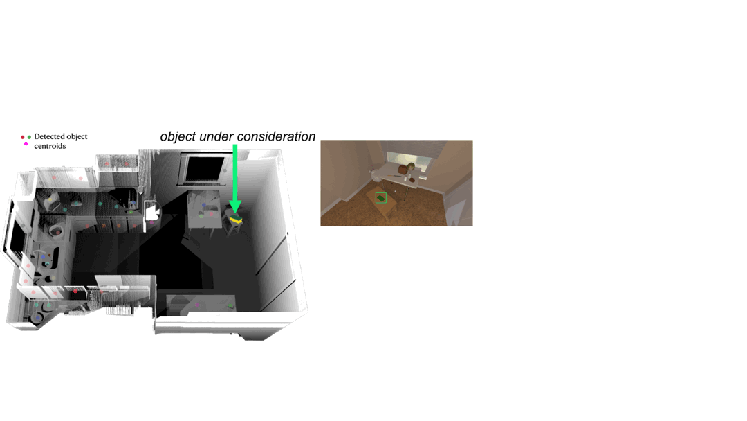
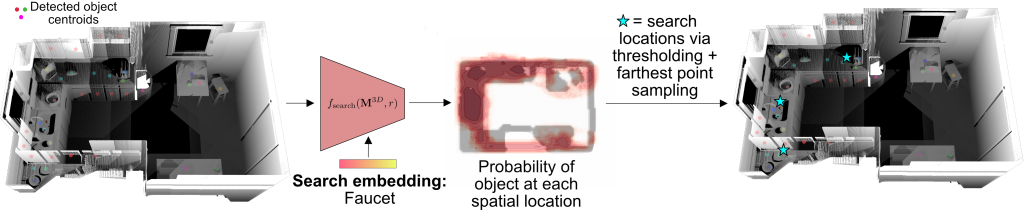
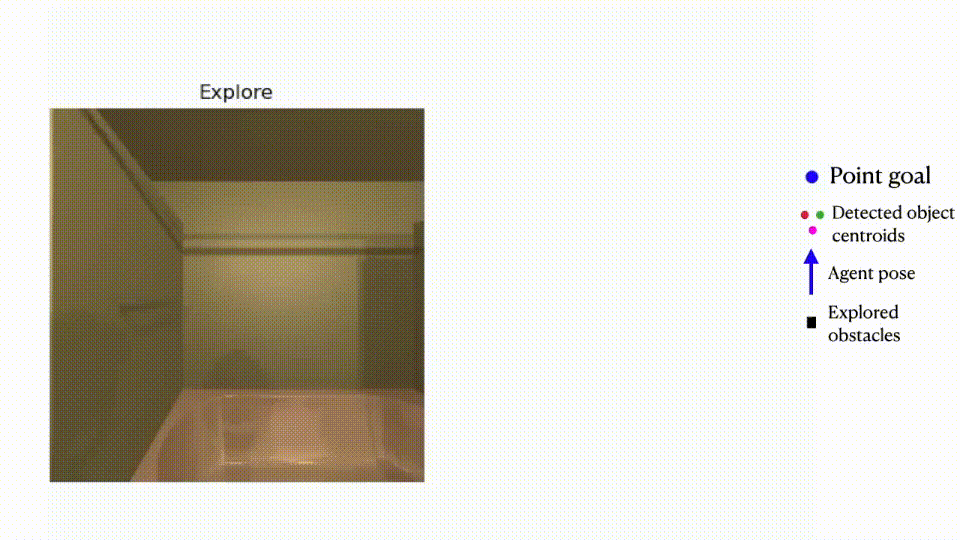
TIDEE tidies up rooms in three phases. In the first phase, TIDEE explores around the room and runs an out of place object detector at each time step until one is identified. Then, TIDEE navigates over to the object, and picks it up. In the second phase, TIDEE uses graph inference in its joint external graph memory and scene graph to infer a plausible receptacle to place the object on within the scene. It then explores the scene guided by a visual search network that suggests where the receptacle may be found if TIDEE has not identified it in a previous time step. For navigation and keeping track objects, TIDEE maintains a obstacle map of the scene and stores in memory the estimated 3D centroids of previously detected objects.

The out of place detector uses visual and relational language features to determine if an object is in or out of place in the context of the scene. The visual features for each object are obtained from an off-the-shelf object detector, and the relational language features are obtained by giving predicted 3D relations of the objects (e.g. next to, supported by, above, etc.) to a pretrained language model. We combine the visual and language features to classify whether each detected object is in or out of place. We find that combining the visual and relational modalities performs best for out of place classification over using a single modality.
To infer where to place an object once it has picked up, TIDEE includes a neural graph module which is trained to predict plausible object placement proposals of objects. The modules works by passing information between the object to be placed, a memory graph encoding plausible contextual relations from training scenes, and a scene graph encoding the object-relation configuration in the current scene. For our memory graph, we take inspiration from “Beyond Categories: The Visual Memex Model for Reasoning About Object Relationships” by Tomasz Malisiewicz and Alexei A. Efros (2009), which models instance-level object features and their relations to provide more complete appearance-based context. Our memory graph consists of the tidy object instances in the training to provide fine-grain contextualization of tidy object placements. We show in the paper that this fine-grain visual and relational information is important for TIDEE to place objects in human-preferred locations.
To search for objects that have not been previously found, TIDEE uses a visual search network that takes as input the semantic obstacle map and a search category and predicts the likelihood of the object being present at each spatial location in the obstacle map. The agent then searches in those likely locations for the object of interest.
Combining all the above modules provides us with a method to be able to detect out of place objects, infer where they should go, search intelligently, and navigate & manipulate effectively. In the next section, we’ll show you how well our agent performs at tidying up rooms.
How good is TIDEE at tidying up?
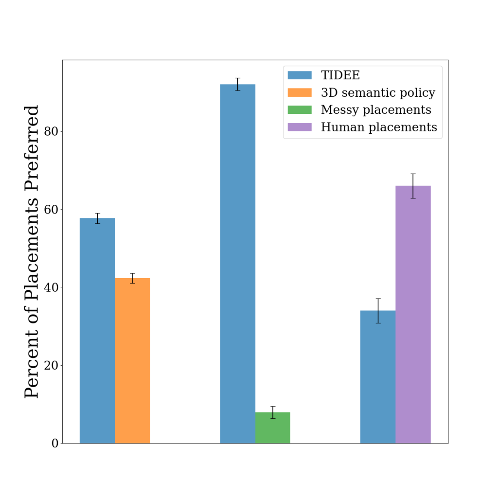
Using a set of messy test scenes that TIDEE has never seen before, we task our agent with reconfiguring the messy room to a tidy state. Since a single object may be tidy in multiple locations within a scene, we evaluate our method by asking humans whether they prefer the placements of TIDEE compared to baseline placements that do not make use of one or more of TIDEE’s commonsense priors. Below we show that TIDEE placements are significantly preferred to the baseline placements, and even competitive with human placements (last row).
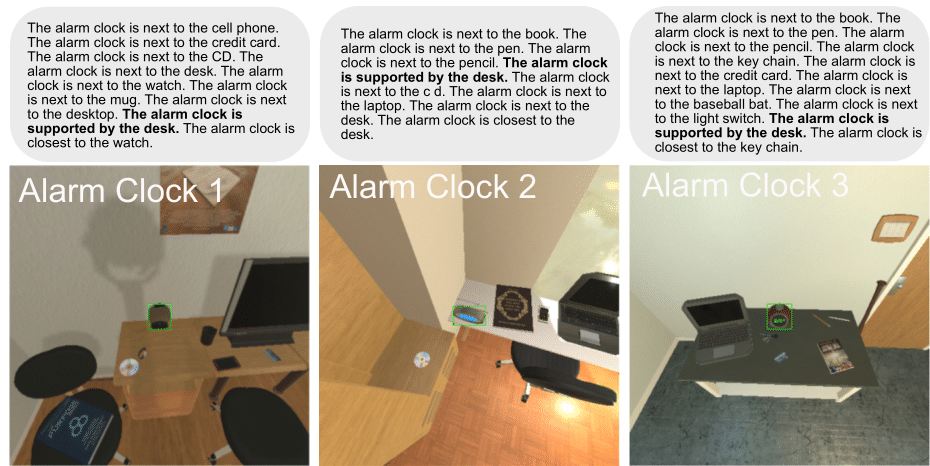
We additionally show that the placements of TIDEE can be customized based on user preferences. For example, based on user input such as “I never want my alarm on the desk”, we can use online learning techniques to change the output from the model that alarm clock being on the desk is out of place (and should be moved). Below we show some examples of locations and relations of alarm clocks that were predicted as being in the correct locations (and not out of place) within the scene after our initial training. However, after doing the user-specified finetuning, our network predicts that the alarm clock on the desk is out of place and should be repositioned.
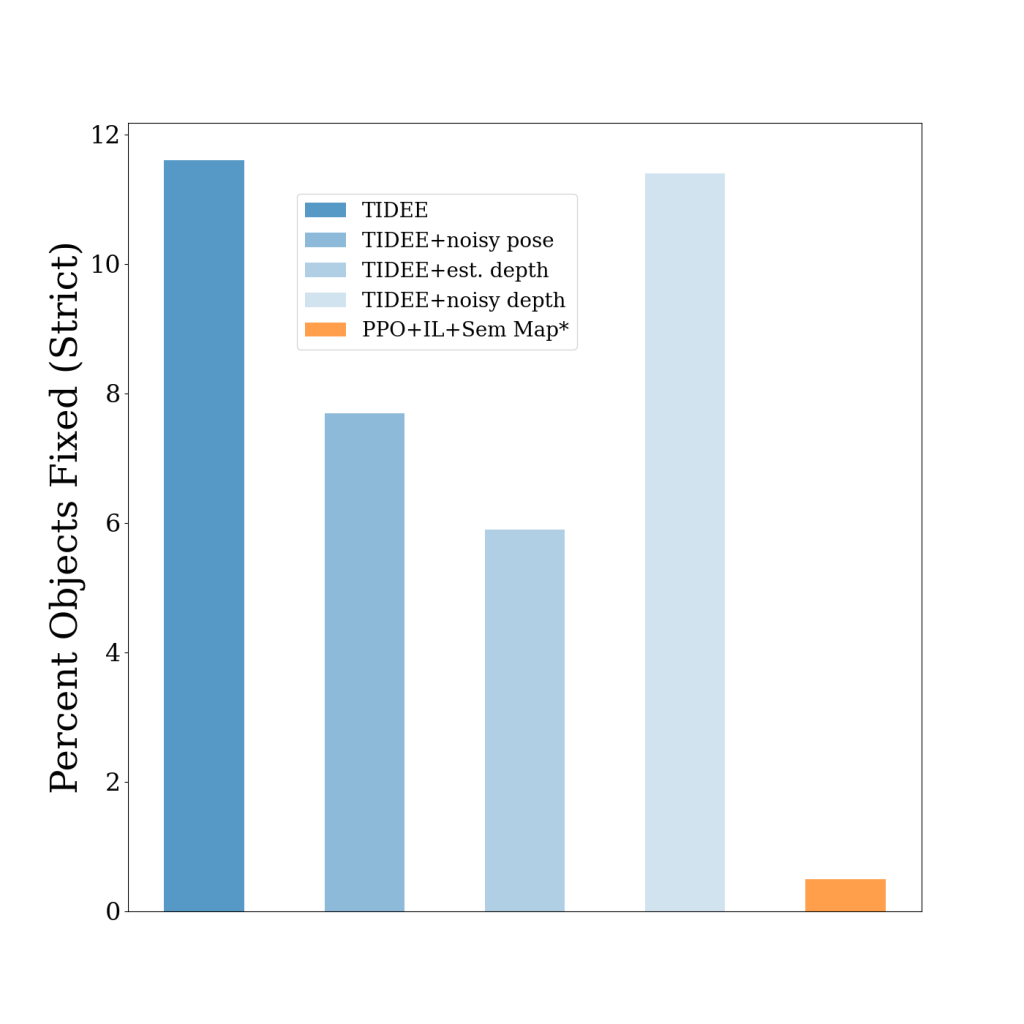
We also show that a simplified version of TIDEE can generalize to task of rearrangement, where the agent sees the original state of the objects, then some of the objects get rearranged to new locations, and the agent must rearrange the objects back to their original state. We outperform the previous state of the art model that utilizes semantic mapping and reinforcement learning, even with noisy sensor measurements.
Summary
In this article, we discussed TIDEE, an embodied agent that uses commonsense reasoning to tidy up novel messy scenes. We introduce a new benchmark to test agents in their ability to clean up messy scenes without any human instruction. To check out our paper, code, and more, please visit our website at https://tidee-agent.github.io/.
Also, feel free to shoot me an email at gsarch@andrew.cmu.edu! I would love to chat!
Beyond automatic differentiation
Derivatives play a central role in optimization and machine learning. By locally approximating a training loss, derivatives guide an optimizer toward lower values of the loss. Automatic differentiation frameworks such as TensorFlow, PyTorch, and JAX are an essential part of modern machine learning, making it feasible to use gradient-based optimizers to train very complex models.
But are derivatives all we need? By themselves, derivatives only tell us how a function behaves on an infinitesimal scale. To use derivatives effectively, we often need to know more than that. For example, to choose a learning rate for gradient descent, we need to know something about how the loss function behaves over a small but finite window. A finite-scale analogue of automatic differentiation, if it existed, could help us make such choices more effectively and thereby speed up training.
In our new paper “Automatically Bounding The Taylor Remainder Series: Tighter Bounds and New Applications“, we present an algorithm called AutoBound that computes polynomial upper and lower bounds on a given function, which are valid over a user-specified interval. We then begin to explore AutoBound’s applications. Notably, we present a meta-optimizer called SafeRate that uses the upper bounds computed by AutoBound to derive learning rates that are guaranteed to monotonically reduce a given loss function, without the need for time-consuming hyperparameter tuning. We are also making AutoBound available as an open-source library.
The AutoBound algorithm
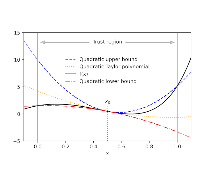
Given a function f and a reference point x0, AutoBound computes polynomial upper and lower bounds on f that hold over a user-specified interval called a trust region. Like Taylor polynomials, the bounding polynomials are equal to f at x0. The bounds become tighter as the trust region shrinks, and approach the corresponding Taylor polynomial as the trust region width approaches zero.
 |
| Automatically-derived quadratic upper and lower bounds on a one-dimensional function f, centered at x0=0.5. The upper and lower bounds are valid over a user-specified trust region, and become tighter as the trust region shrinks. |
Like automatic differentiation, AutoBound can be applied to any function that can be implemented using standard mathematical operations. In fact, AutoBound is a generalization of Taylor mode automatic differentiation, and is equivalent to it in the special case where the trust region has a width of zero.
To derive the AutoBound algorithm, there were two main challenges we had to address:
- We had to derive polynomial upper and lower bounds for various elementary functions, given an arbitrary reference point and arbitrary trust region.
- We had to come up with an analogue of the chain rule for combining these bounds.
Bounds for elementary functions
For a variety of commonly-used functions, we derive optimal polynomial upper and lower bounds in closed form. In this context, “optimal” means the bounds are as tight as possible, among all polynomials where only the maximum-degree coefficient differs from the Taylor series. Our theory applies to elementary functions, such as exp and log, and common neural network activation functions, such as ReLU and Swish. It builds upon and generalizes earlier work that applied only to quadratic bounds, and only for an unbounded trust region.
 |
| Optimal quadratic upper and lower bounds on the exponential function, centered at x0=0.5 and valid over the interval [0, 2]. |
A new chain rule
To compute upper and lower bounds for arbitrary functions, we derived a generalization of the chain rule that operates on polynomial bounds. To illustrate the idea, suppose we have a function that can be written as
f(x) = g(h(x))
and suppose we already have polynomial upper and lower bounds on g and h. How do we compute bounds on f?
The key turns out to be representing the upper and lower bounds for a given function as a single polynomial whose highest-degree coefficient is an interval rather than a scalar. We can then plug the bound for h into the bound for g, and convert the result back to a polynomial of the same form using interval arithmetic. Under suitable assumptions about the trust region over which the bound on g holds, it can be shown that this procedure yields the desired bound on f.
 |
| The interval polynomial chain rule applied to the functions h(x) = sqrt(x) and g(y) = exp(y), with x0=0.25 and trust region [0, 0.5]. |
Our chain rule applies to one-dimensional functions, but also to multivariate functions, such as matrix multiplications and convolutions.
Propagating bounds
Using our new chain rule, AutoBound propagates interval polynomial bounds through a computation graph from the inputs to the outputs, analogous to forward-mode automatic differentiation.
 |
| Forward propagation of interval polynomial bounds for the function f(x) = exp(sqrt(x)). We first compute (trivial) bounds on x, then use the chain rule to compute bounds on sqrt(x) and exp(sqrt(x)). |
To compute bounds on a function f(x), AutoBound requires memory proportional to the dimension of x. For this reason, practical applications apply AutoBound to functions with a small number of inputs. However, as we will see, this does not prevent us from using AutoBound for neural network optimization.
Automatically deriving optimizers, and other applications
What can we do with AutoBound that we couldn’t do with automatic differentiation alone?
Among other things, AutoBound can be used to automatically derive problem-specific, hyperparameter-free optimizers that converge from any starting point. These optimizers iteratively reduce a loss by first using AutoBound to compute an upper bound on the loss that is tight at the current point, and then minimizing the upper bound to obtain the next point.
 |
| Minimizing a one-dimensional logistic regression loss using quadratic upper bounds derived automatically by AutoBound. |
Optimizers that use upper bounds in this way are called majorization-minimization (MM) optimizers. Applied to one-dimensional logistic regression, AutoBound rederives an MM optimizer first published in 2009. Applied to more complex problems, AutoBound derives novel MM optimizers that would be difficult to derive by hand.
We can use a similar idea to take an existing optimizer such as Adam and convert it to a hyperparameter-free optimizer that is guaranteed to monotonically reduce the loss (in the full-batch setting). The resulting optimizer uses the same update direction as the original optimizer, but modifies the learning rate by minimizing a one-dimensional quadratic upper bound derived by AutoBound. We refer to the resulting meta-optimizer as SafeRate.
 |
| Performance of SafeRate when used to train a single-hidden-layer neural network on a subset of the MNIST dataset, in the full-batch setting. |
Using SafeRate, we can create more robust variants of existing optimizers, at the cost of a single additional forward pass that increases the wall time for each step by a small factor (about 2x in the example above).
In addition to the applications just discussed, AutoBound can be used for verified numerical integration and to automatically prove sharper versions of Jensen’s inequality, a fundamental mathematical inequality used frequently in statistics and other fields.
Improvement over classical bounds
Bounding the Taylor remainder term automatically is not a new idea. A classical technique produces degree k polynomial bounds on a function f that are valid over a trust region [a, b] by first computing an expression for the kth derivative of f (using automatic differentiation), then evaluating this expression over [a,b] using interval arithmetic.
While elegant, this approach has some inherent limitations that can lead to very loose bounds, as illustrated by the dotted blue lines in the figure below.
 |
| Quadratic upper and lower bounds on the loss of a multi-layer perceptron with two hidden layers, as a function of the initial learning rate. The bounds derived by AutoBound are much tighter than those obtained using interval arithmetic evaluation of the second derivative. |
Looking forward
Taylor polynomials have been in use for over three hundred years, and are omnipresent in numerical optimization and scientific computing. Nevertheless, Taylor polynomials have significant limitations, which can limit the capabilities of algorithms built on top of them. Our work is part of a growing literature that recognizes these limitations and seeks to develop a new foundation upon which more robust algorithms can be built.
Our experiments so far have only scratched the surface of what is possible using AutoBound, and we believe it has many applications we have not discovered. To encourage the research community to explore such possibilities, we have made AutoBound available as an open-source library built on top of JAX. To get started, visit our GitHub repo.
Acknowledgements
This post is based on joint work with Josh Dillon. We thank Alex Alemi and Sergey Ioffe for valuable feedback on an earlier draft of the post.
The science of price experiments in the Amazon Store
The requirement that at any given time, all customers see the same prices for the same products necessitates innovation in the design of A/B experiments.Read More
Accelerated Generative Diffusion Models with PyTorch 2
TL;DR: PyTorch 2.0 nightly offers out-of-the-box performance improvement for Generative Diffusion models by using the new torch.compile() compiler and optimized implementations of Multihead Attention integrated with PyTorch 2.
Introduction
A large part of the recent progress in Generative AI came from denoising diffusion models, which allow producing high quality images and videos from text prompts. This family includes Imagen, DALLE, Latent Diffusion, and others. However, all models in this family share a common drawback: generation is rather slow, due to the iterative nature of the sampling process by which the images are produced. This makes it important to optimize the code running inside the sampling loop.
We took an open source implementation of a popular text-to-image diffusion model as a starting point and accelerated its generation using two optimizations available in PyTorch 2: compilation and fast attention implementation. Together with a few minor memory processing improvements in the code these optimizations give up to 49% inference speedup relative to the original implementation without xFormers, and 39% inference speedup relative to using the original code with xFormers (excluding the compilation time), depending on the GPU architecture and batch size. Importantly, the speedup comes without a need to install xFormers or any other extra dependencies.
The table below shows the improvement in runtime between the original implementation with xFormers installed and our optimized version with PyTorch-integrated memory efficient attention (originally developed for and released in the xFormers library) and PyTorch compilation. The compilation time is excluded.
Runtime improvement in % compared to original+xFormers
See the absolute runtime numbers in section “Benchmarking setup and results summary”
| GPU | Batch size 1 | Batch size 2 | Batch size 4 |
| P100 (no compilation) | -3.8 | 0.44 | 5.47 |
| T4 | 2.12 | 10.51 | 14.2 |
| A10 | -2.34 | 8.99 | 10.57 |
| V100 | 18.63 | 6.39 | 10.43 |
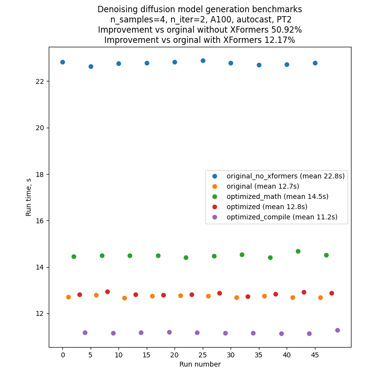
| A100 | 38.5 | 20.33 | 12.17 |
One can notice the following:
- The improvements are significant for powerful GPUs like A100 and V100. For those GPUs the improvement is most pronounced for batch size 1
- For less powerful GPUs we observe smaller speedups (or in two cases slight regressions). The batch size trend is reversed here: improvement is larger for larger batches
In the following sections we describe the applied optimizations and provide detailed benchmarking data, comparing the generation time with various optimization features on/off.
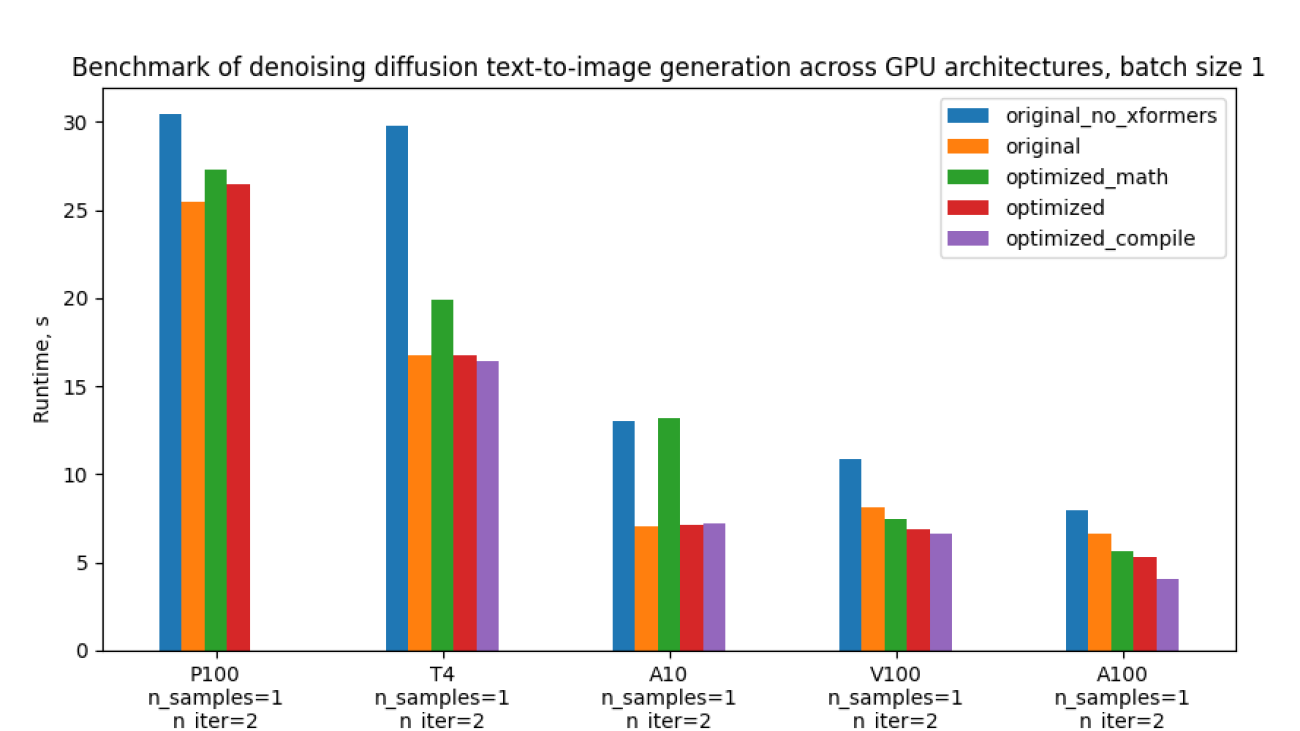
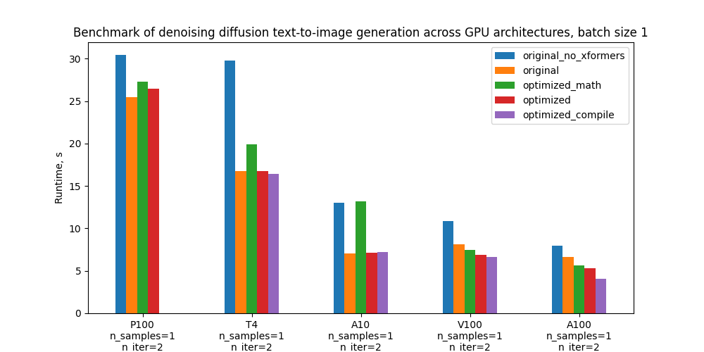
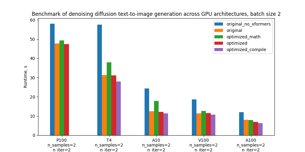
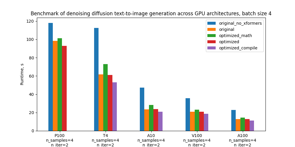
Specifically, we benchmark 5 configurations and the plots below compare their absolute performance for different GPUs and batch sizes. For definitions of these configurations see section “Benchmarking setup and results”.
Optimizations
Here we’ll go into more detail about the optimizations introduced into the model code. These optimizations rely on features of PyTorch 2.0 which has been released recently.
Optimized Attention
One part of the code which we optimized is the scaled dot-product attention. Attention is known to be a heavy operation: naive implementation materializes the attention matrix, leading to time and memory complexity quadratic in sequence length. It is common for diffusion models to use attention (CrossAttention) as part of Transformer blocks in multiple parts of the U-Net. Since the U-Net runs at every sampling step, this becomes a critical point to optimize. Instead of custom attention implementation one can use torch.nn.MultiheadAttention, which in PyTorch 2 has optimized attention implementation is integrated into it. This optimization schematically boils down to the following pseudocode:
class CrossAttention(nn.Module):
    def __init__(self, ...):
        # Create matrices: Q, K, V, out_proj
        ...
    def forward(self, x, context=None, mask=None):
       # Compute out = SoftMax(Q*K/sqrt(d))V
       # Return out_proj(out)
       …
gets replaced with
class CrossAttention(nn.Module):
    def __init__(self, ...):
        self.mha = nn.MultiheadAttention(...)
    def forward(self, x, context):
	return self.mha(x, context, context)
The optimized implementation of attention was available already in PyTorch 1.13 (see here) and widely adopted (see e.g. HuggingFace transformers library example). In particular, it integrates memory-efficient attention from the xFormers library and flash attention from https://arxiv.org/abs/2205.14135. PyTorch 2.0 expands this to additional attention functions such as cross attention and custom kernels for further acceleration, making it applicable to diffusion models.
Flash attention is available on GPUs with compute capability SM 7.5 or SM 8.x – for example, on T4, A10, and A100, which are included in our benchmark (you can check compute capability of each NVIDIA GPU here). However, in our tests on A100 the memory efficient attention performed better than flash attention for the particular case of diffusion models, due to the small number of attention heads and small batch size. PyTorch understands this and in this case chooses memory efficient attention over flash attention when both are available (see the logic here). For full control over the attention backends (memory-efficient attention, flash attention, “vanilla math”, or any future ones), power users can enable and disable them manually with the help of the context manager torch.backends.cuda.sdp_kernel.
Compilation
Compilation is a new feature of PyTorch 2.0, enabling significant speedups with a very simple user experience. To invoke the default behavior, simply wrap a PyTorch module or a function into torch.compile:
model = torch.compile(model)
PyTorch compiler then turns Python code into a set of instructions which can be executed efficiently without Python overhead. The compilation happens dynamically the first time the code is executed. With the default behavior, under the hood PyTorch utilized TorchDynamo to compile the code and TorchInductor to further optimize it. See this tutorial for more details.
Although the one-liner above is enough for compilation, certain modifications in the code can squeeze a larger speedup. In particular, one should avoid so-called graph breaks – places in the code which PyTorch can’t compile. As opposed to previous PyTorch compilation approaches (like TorchScript), PyTorch 2 compiler doesn’t break in this case. Instead it falls back on eager execution – so the code runs, but with reduced performance. We introduced a few minor changes to the model code to get rid of graph breaks. This included eliminating functions from libraries not supported by the compiler, such as inspect.isfunction and einops.rearrange. See this doc to learn more about graph breaks and how to eliminate them.
Theoretically, one can apply torch.compile on the whole diffusion sampling loop. However, in practice it is enough to just compile the U-Net. The reason is that torch.compile doesn’t yet have a loop analyzer and would recompile the code for each iteration of the sampling loop. Moreover, compiled sampler code is likely to generate graph breaks – so one would need to adjust it if one wants to get a good performance from the compiled version.
Note that compilation requires GPU compute capability >= SM 7.0 to run in non-eager mode. This covers all GPUs in our benchmarks – T4, V100, A10, A100 – except for P100 (see the full list).
Other optimizations
In addition, we have improved efficiency of GPU memory operations by eliminating some common pitfalls, e.g. creating a tensor on GPU directly rather than creating it on CPU and later moving to GPU. The places where such optimizations were necessary were determined by line-profiling and looking at CPU/GPU traces and Flame Graphs.
Benchmarking setup and results summary
We have two versions of code to compare: original and optimized. On top of this, several optimization features (xFormers, PyTorch memory efficient attention, compilation) can be turned on/off. Overall, as mentioned in the introduction, we will be benchmarking 5 configurations:
- Original code without xFormers
- Original code with xFormers
- Optimized code with vanilla math attention backend and no compilation
- Optimized code with memory-efficient attention backend and no compilation
- Optimized code with memory-efficient attention backend and compilation
As the original version we took the version of the code which uses PyTorch 1.12 and a custom implementation of attention. The optimized version uses nn.MultiheadAttention in CrossAttention and PyTorch 2.0.0.dev20230111+cu117. It also has a few other minor optimizations in PyTorch-related code.
The table below shows runtime of each version of the code in seconds, and the percentage improvement compared to the _original with xFormers. _The compilation time is excluded.
Runtimes for batch size 1. In parenthesis – relative improvement with respect to the “Original with xFormers” row
| Configuration | P100 | T4 | A10 | V100 | A100 |
| Original without xFormers | 30.4s (-19.3%) | 29.8s (-77.3%) | 13.0s (-83.9%) | 10.9s (-33.1%) | 8.0s (-19.3%) |
| Original with xFormers | 25.5s (0.0%) | 16.8s (0.0%) | 7.1s (0.0%) | 8.2s (0.0%) | 6.7s (0.0%) |
| Optimized with vanilla math attention, no compilation | 27.3s (-7.0%) | 19.9s (-18.7%) | 13.2s (-87.2%) | 7.5s (8.7%) | 5.7s (15.1%) |
| Optimized with mem. efficient attention, no compilation | 26.5s (-3.8%) | 16.8s (0.2%) | 7.1s (-0.8%) | 6.9s (16.0%) | 5.3s (20.6%) |
| Optimized with mem. efficient attention and compilation | – | 16.4s (2.1%) | 7.2s (-2.3%) | 6.6s (18.6%) | 4.1s (38.5%) |
Runtimes for batch size 2
| Configuration | P100 | T4 | A10 | V100 | A100 |
| Original without xFormers | 58.0s (-21.6%) | 57.6s (-84.0%) | 24.4s (-95.2%) | 18.6s (-63.0%) | 12.0s (-50.6%) |
| Original with xFormers | 47.7s (0.0%) | 31.3s (0.0%) | 12.5s (0.0%) | 11.4s (0.0%) | 8.0s (0.0%) |
| Optimized with vanilla math attention, no compilation | 49.3s (-3.5%) | 37.9s (-21.0%) | 17.8s (-42.2%) | 12.7s (-10.7%) | 7.8s (1.8%) |
| Optimized with mem. efficient attention, no compilation | 47.5s (0.4%) | 31.2s (0.5%) | 12.2s (2.6%) | 11.5s (-0.7%) | 7.0s (12.6%) |
| Optimized with mem. efficient attention and compilation | – | 28.0s (10.5%) | 11.4s (9.0%) | 10.7s (6.4%) | 6.4s (20.3%) |
Runtimes for batch size 4
| Configuration | P100 | T4 | A10 | V100 | A100 |
| Original without xFormers | 117.9s (-20.0%) | 112.4s (-81.8%) | 47.2s (-101.7%) | 35.8s (-71.9%) | 22.8s (-78.9%) |
| Original with xFormers | 98.3s (0.0%) | 61.8s (0.0%) | 23.4s (0.0%) | 20.8s (0.0%) | 12.7s (0.0%) |
| Optimized with vanilla math attention, no compilation | 101.1s (-2.9%) | 73.0s (-18.0%) | 28.3s (-21.0%) | 23.3s (-11.9%) | 14.5s (-13.9%) |
| Optimized with mem. efficient attention, no compilation | 92.9s (5.5%) | 61.1s (1.2%) | 23.9s (-1.9%) | 20.8s (-0.1%) | 12.8s (-0.9%) |
| Optimized with mem. efficient attention and compilation | – | 53.1s (14.2%) | 20.9s (10.6%) | 18.6s (10.4%) | 11.2s (12.2%) |
To minimize fluctuations and external influence on the performance of the benchmarked code, we ran each version of the code one after another, and then repeated this sequence 10 times: A, B, C, D, E, A, B, … So the results of a typical run would look like the one in the picture below.. Note that one shouldn’t rely on comparison of absolute run times between different graphs, but comparison of run times_ inside_ one graph is pretty reliable, thanks to our benchmarking setup.
Each run of text-to-image generation script produces several batches, the number of which is regulated by the CLI parameter --n_iter. In the benchmarks we used n_iter = 2, but introduced an additional “warm-up” iteration, which doesn’t contribute to the run time. This was necessary for the runs with compilation, because compilation happens the first time the code runs, and so the first iteration is much longer than all subsequent. To make comparison fair, we also introduced this additional “warm-up” iteration to all other runs.
The numbers in the table above are for number of iterations 2 (plus a “warm-up one”), prompt ”A photo”, seed 1, PLMS sampler, and autocast turned on.
Benchmarks were done using P100, V100, A100, A10 and T4 GPUs. The T4 benchmarks were done in Google Colab Pro. The A10 benchmarks were done on g5.4xlarge AWS instances with 1 GPU.
Conclusions and next steps
We have shown that new features of PyTorch 2 – compiler and optimized attention implementation – give performance improvements exceeding or comparable with what previously required installation of an external dependency (xFormers). PyTorch achieved this, in particular, by integrating memory efficient attention from xFormers into its codebase. This is a significant improvement for user experience, given that xFormers, being a state-of-the-art library, in many scenarios requires custom installation process and long builds.
There are a few natural directions in which this work can be continued:
- The optimizations we implemented and described here are only benchmarked for text-to-image inference so far. It would be interesting to see how they affect training performance. PyTorch compilation can be directly applied to training; enabling training with PyTorch optimized attention is on the roadmap
- We intentionally minimized changes to the original model code. Further profiling and optimization can probably bring more improvements
- At the moment compilation is applied only to the U-Net model inside the sampler. Since there is a lot happening outside of U-Net (e.g. operations directly in the sampling loop), it would be beneficial to compile the whole sampler. However, this would require analysis of the compilation process to avoid recompilation at every sampling step
- Current code only applies compilation within the PLMS sampler, but it should be trivial to extend it to other samplers
- Besides text-to-image generation, diffusion models are also applied to other tasks – image-to-image and inpainting. It would be interesting to measure how their performance improves from PyTorch 2 optimizations
See if you can increase performance of open source diffusion models using the methods we described, and share the results!
Resources
- PyTorch 2.0 overview, which has a lot of information on
torch.compile:https://pytorch.org/get-started/pytorch-2.0/ - Tutorial on
torch.compile: https://pytorch.org/tutorials/intermediate/torch_compile_tutorial.html - General compilation troubleshooting: https://pytorch.org/docs/master/dynamo/troubleshooting.html
- Details on graph breaks: https://pytorch.org/docs/master/dynamo/faq.html#identifying-the-cause-of-a-graph-break
- Details on guards: https://pytorch.org/docs/master/dynamo/guards-overview.html
- Video deep dive on TorchDynamo https://www.youtube.com/watch?v=egZB5Uxki0I
- Tutorial on optimized attention in PyTorch 1.12: https://pytorch.org/tutorials/beginner/bettertransformer_tutorial.html
Acknowledgements
We would like to thank Geeta Chauhan, Natalia Gimelshein, Patrick Labatut, Bert Maher, Mark Saroufim, Michael Voznesensky and Francisco Massa for their valuable advice and early feedback on the text.
Special thanks to Yudong Tao initiating the work on using PyTorch native attention in diffusion models.

Robotic deep RL at scale: Sorting waste and recyclables with a fleet of robots
Reinforcement learning (RL) can enable robots to learn complex behaviors through trial-and-error interaction, getting better and better over time. Several of our prior works explored how RL can enable intricate robotic skills, such as robotic grasping, multi-task learning, and even playing table tennis. Although robotic RL has come a long way, we still don’t see RL-enabled robots in everyday settings. The real world is complex, diverse, and changes over time, presenting a major challenge for robotic systems. However, we believe that RL should offer us an excellent tool for tackling precisely these challenges: by continually practicing, getting better, and learning on the job, robots should be able to adapt to the world as it changes around them.
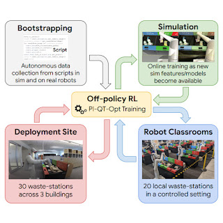
In “Deep RL at Scale: Sorting Waste in Office Buildings with a Fleet of Mobile Manipulators”, we discuss how we studied this problem through a recent large-scale experiment, where we deployed a fleet of 23 RL-enabled robots over two years in Google office buildings to sort waste and recycling. Our robotic system combines scalable deep RL from real-world data with bootstrapping from training in simulation and auxiliary object perception inputs to boost generalization, while retaining the benefits of end-to-end training, which we validate with 4,800 evaluation trials across 240 waste station configurations.
Problem setup
When people don’t sort their trash properly, batches of recyclables can become contaminated and compost can be improperly discarded into landfills. In our experiment, a robot roamed around an office building searching for “waste stations” (bins for recyclables, compost, and trash). The robot was tasked with approaching each waste station to sort it, moving items between the bins so that all recyclables (cans, bottles) were placed in the recyclable bin, all the compostable items (cardboard containers, paper cups) were placed in the compost bin, and everything else was placed in the landfill trash bin. Here is what that looks like:
This task is not as easy as it looks. Just being able to pick up the vast variety of objects that people deposit into waste bins presents a major learning challenge. Robots also have to identify the appropriate bin for each object and sort them as quickly and efficiently as possible. In the real world, the robots can encounter a variety of situations with unique objects, like the examples from real office buildings below:
 |
Learning from diverse experience
Learning on the job helps, but before even getting to that point, we need to bootstrap the robots with a basic set of skills. To this end, we use four sources of experience: (1) a set of simple hand-designed policies that have a very low success rate, but serve to provide some initial experience, (2) a simulated training framework that uses sim-to-real transfer to provide some initial bin sorting strategies, (3) “robot classrooms” where the robots continually practice at a set of representative waste stations, and (4) the real deployment setting, where robots practice in real office buildings with real trash.
 |
| A diagram of RL at scale. We bootstrap policies from data generated with a script (top-left). We then train a sim-to-real model and generate additional data in simulation (top-right). At each deployment cycle, we add data collected in our classrooms (bottom-right). We further deploy and collect data in office buildings (bottom-left). |
Our RL framework is based on QT-Opt, which we previously applied to learn bin grasping in laboratory settings, as well as a range of other skills. In simulation, we bootstrap from simple scripted policies and use RL, with a CycleGAN-based transfer method that uses RetinaGAN to make the simulated images appear more life-like.
From here, it’s off to the classroom. While real-world office buildings can provide the most representative experience, the throughput in terms of data collection is limited — some days there will be a lot of trash to sort, some days not so much. Our robots collect a large portion of their experience in “robot classrooms.” In the classroom shown below, 20 robots practice the waste sorting task:
While these robots are training in the classrooms, other robots are simultaneously learning on the job in 3 office buildings, with 30 waste stations:
Sorting performance
In the end, we gathered 540k trials in the classrooms and 32.5k trials from deployment. Overall system performance improved as more data was collected. We evaluated our final system in the classrooms to allow for controlled comparisons, setting up scenarios based on what the robots saw during deployment. The final system could accurately sort about 84% of the objects on average, with performance increasing steadily as more data was added. In the real world, we logged statistics from three real-world deployments between 2021 and 2022, and found that our system could reduce contamination in the waste bins by between 40% and 50% by weight. Our paper provides further insights on the technical design, ablations studying various design decisions, and more detailed statistics on the experiments.
Conclusion and future work
Our experiments showed that RL-based systems can enable robots to address real-world tasks in real office environments, with a combination of offline and online data enabling robots to adapt to the broad variability of real-world situations. At the same time, learning in more controlled “classroom” environments, both in simulation and in the real world, can provide a powerful bootstrapping mechanism to get the RL “flywheel” spinning to enable this adaptation. There is still a lot left to do: our final RL policies do not succeed every time, and larger and more powerful models will be needed to improve their performance and extend them to a broader range of tasks. Other sources of experience, including from other tasks, other robots, and even Internet videos may serve to further supplement the bootstrapping experience that we obtained from simulation and classrooms. These are exciting problems to tackle in the future. Please see the full paper here, and the supplementary video materials on the project webpage.
Acknowledgements
This research was conducted by multiple researchers at Robotics at Google and Everyday Robots, with contributions from Alexander Herzog, Kanishka Rao, Karol Hausman, Yao Lu, Paul Wohlhart, Mengyuan Yan, Jessica Lin, Montserrat Gonzalez Arenas, Ted Xiao, Daniel Kappler, Daniel Ho, Jarek Rettinghouse, Yevgen Chebotar, Kuang-Huei Lee, Keerthana Gopalakrishnan, Ryan Julian, Adrian Li, Chuyuan Kelly Fu, Bob Wei, Sangeetha Ramesh, Khem Holden, Kim Kleiven, David Rendleman, Sean Kirmani, Jeff Bingham, Jon Weisz, Ying Xu, Wenlong Lu, Matthew Bennice, Cody Fong, David Do, Jessica Lam, Yunfei Bai, Benjie Holson, Michael Quinlan, Noah Brown, Mrinal Kalakrishnan, Julian Ibarz, Peter Pastor, Sergey Levine and the entire Everyday Robots team.
Angler: Helping Machine Translation Practitioners Prioritize Model Improvements
*=Authors contributed equally
Machine learning (ML) models can fail in unexpected ways in the real world, but not all model failures are equal. With finite time and resources, ML practitioners are forced to prioritize their model debugging and improvement efforts. Through interviews with 13 ML practitioners at Apple, we found that practitioners construct small targeted test sets to estimate an error’s nature, scope, and impact on users. We built on this insight in a case study with machine translation models, and developed Angler, an interactive visual analytics tool to help practitioners…Apple Machine Learning Research
Hunting speculative information leaks with Revizor
Spectre and Meltdown are two security vulnerabilities that affect the vast majority of CPUs in use today. CPUs, or central processing units, act as the brains of a computer, directing the functions of its other components. By targeting a feature of the CPU implementation that optimizes performance, attackers could access sensitive data previously considered inaccessible.
For example, Spectre exploits speculative execution—an aggressive strategy for increasing processing speed by postponing certain security checks. But it turns out that before the CPU performs the security check, attackers might have already extracted secrets via so-called side-channels. This vulnerability went undetected for years before it was discovered and mitigated in 2018. Security researchers warned that thieves could use it to target countless computers, phones and mobile devices. Researchers began hunting for more vulnerabilities, and they continue to find them. But this process is manual and progress came slowly. With no tools available to help them search, researchers had to analyze documentation, read through patents, and experiment with different CPU generations.
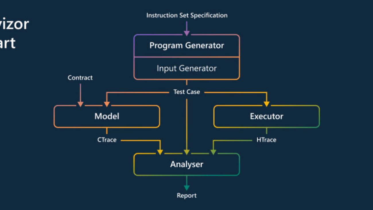
A group of researchers from Microsoft and academic partners began exploring a method for systematically finding and analyzing CPU vulnerabilities. This effort would produce a tool called Revizor (REV-izz-or), which automatically detects microarchitectural leakage in CPUs—with no prior knowledge about the internal CPU components. Revizor achieves this by differentiating between expected and unexpected information leaks on the CPU.
Spotlight: Microsoft Research Podcast

AI Frontiers: The Physics of AI with Sébastien Bubeck
What is intelligence? How does it emerge and how do we measure it? Ashley Llorens and machine learning theorist Sébastian Bubeck discuss accelerating progress in large-scale AI and early experiments with GPT-4.
The Revizor process begins by describing what is expected from the CPU in a so-called “leakage contract.” Revizor then searches the CPU to find any violations of this contract. It creates random programs, runs them on the CPU, records the information they expose, and compares the information with the contract. When it finds a mismatch that violates the contract, it reports it as a potential vulnerability.
Details were published in 2022 in the paper: Revizor: Testing Black-box CPUs against Speculation Contracts.
To demonstrate Revizor’s effectiveness, the researchers tested a handful of commercial CPUs and found several known vulnerabilities, including Spectre, MDS, and LVI, as well as several previously unknown variants.
However, the search was still slow, which hindered the discovery of entirely new classes of leaks. The team identified the root causes of the performance limitations, and proposed techniques to overcome them, improving the testing speed by up to two orders of magnitude. The improvements are described in a newly published paper: Hide and Seek with Spectres: Efficient discovery of speculative information leaks with random testing.
These improvements supported a testing campaign of unprecedented depth on Intel and AMD CPUs. In the process, the researchers found two types of previously unknown speculative leaks (affecting string comparison and division) that had escaped previous analyses—both manual and automated. These results show that work which previously required persistent hacking and painstaking manual labor can now be automated and rapidly accelerated.
The team began working with the Microsoft Security Response Center and hardware vendors, and together they continue to find vulnerabilities so they can be closed before they are discovered by hackers—thereby protecting customers from risk.
Revizor is part of Project Venice, which investigates novel mechanisms for the secure sharing and partitioning of computing resources, together with techniques for specifying and rigorously validating their resilience to side-channel attacks.
The post Hunting speculative information leaks with Revizor appeared first on Microsoft Research.