Detect real and live users and deter bad actors using Amazon Rekognition Face Liveness
Financial services, the gig economy, telco, healthcare, social networking, and other customers use face verification during online onboarding, step-up authentication, age-based access restriction, and bot detection. These customers verify user identity by matching the user’s face in a selfie captured by a device camera with a government-issued identity card photo or preestablished profile photo. They also estimate the user’s age using facial analysis before allowing access to age-restricted content. However, bad actors increasingly deploy spoof attacks using the user’s face images or videos posted publicly, captured secretly, or created synthetically to gain unauthorized access to the user’s account. To deter this fraud, as well as reduce the costs associated with it, customers need to add liveness detection before face matching or age estimation is performed in their face verification workflow to confirm that the user in front of the camera is a real and live person.
We are excited to introduce Amazon Rekognition Face Liveness to help you easily and accurately deter fraud during face verification. In this post, we start with an overview of the Face Liveness feature, its use cases, and the end-user experience; provide an overview of its spoof detection capabilities; and show how you can add Face Liveness to your web and mobile applications.
Face Liveness overview
Today, customers detect liveness using various solutions. Some customers use open-source or commercial facial landmark detection machine learning (ML) models in their web and mobile applications to check if users correctly perform specific gestures such as smiling, nodding, shaking their head, blinking their eyes, or opening their mouth. These solutions are costly to build and maintain, fail to deter advanced spoof attacks performed using physical 3D masks or injected videos, and require high user effort to complete. Some customers use third-party face liveness features that can only detect spoof attacks presented to the camera (such as printed or digital photos or videos on a screen), which work well for users in select geographies, and are often completely customer-managed. Lastly, some customer solutions rely on hardware-based infrared and other sensors in phone or computer cameras to detect face liveness, but these solutions are costly, hardware-specific, and work only for users with select high-end devices.
With Face Liveness, you can detect in seconds that real users, and not bad actors using spoofs, are accessing your services. Face Liveness includes these key features:
- Analyzes a short selfie video from the user in real time to detect whether the user is real or a spoof
- Returns a liveness confidence score—a metric for the confidence level from 0–100 that indicates the probability for a person being real and live
- Returns a high-quality reference image—a selfie frame with quality checks that can be used for downstream Amazon Rekognition face matching or age estimation analysis
- Returns up to four audit images—frames from the selfie video that can be used for maintaining audit trails
- Detects spoofs presented to the camera, such as a printed photo, digital photo, digital video, or 3D mask, as well as spoofs that bypass the camera, such as a pre-recorded or deepfake video
- Can easily be added to applications running on most devices with a front-facing camera using open-source pre-built AWS Amplify UI components
In addition, no infrastructure management, hardware-specific implementation, or ML expertise is required. The feature automatically scales up or down in response to demand, and you only pay for the face liveness checks you perform. Face Liveness uses ML models trained on diverse datasets to provide high accuracy across user skin tones, ancestries, and devices.
Use cases
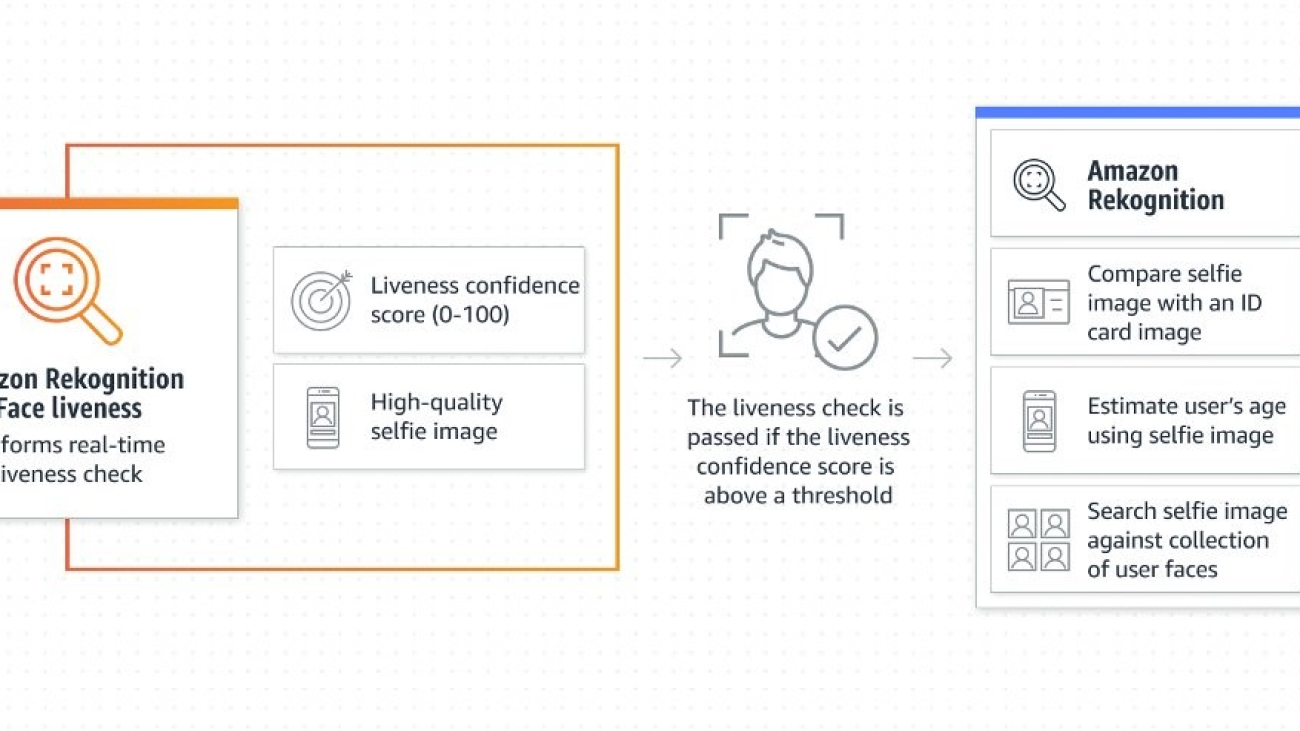
The following diagram illustrates a typical workflow using Face Liveness.

You can use Face Liveness in the following user verification workflows:
- User onboarding – You can reduce fraudulent account creation on your service by validating new users with Face Liveness before downstream processing. For example, a financial services customer can use Face Liveness to detect a real and live user and then perform face matching to check that this is the right user prior to opening an online account. This can deter a bad actor using social media pictures of another person to open fraudulent bank accounts.
- Step-up authentication – You can strengthen the verification of high-value user activities on your services, such as device change, password change, and money transfers, with Face Liveness before the activity is performed. For example, a ride-sharing or food-delivery customer can use Face Liveness to detect a real and live user and then perform face matching using an established profile picture to verify a driver’s or delivery associate’s identity before a ride or delivery to promote safety. This can deter unauthorized delivery associates and drivers from engaging with end-users.
- User age verification – You can deter underage users from accessing restricted online content. For example, online tobacco retailers or online gambling customers can use Face Liveness to detect a real and live user and then perform age estimation using facial analysis to verify the user’s age before granting them access to the service content. This can deter an underage user from using their parent’s credit cards or photo and gaining access to harmful or inappropriate content.
- Bot detection – You can avoid bots from engaging with your service by using Face Liveness in place of “real human” captcha checks. For example, social media customers can use Face Liveness for posing real human checks to keep bots at bay. This significantly increases the cost and effort required by users driving bot activity because key bot actions now need to pass a face liveness check.
End-user experience
When end-users need to onboard or authenticate themselves on your application, Face Liveness provides the user interface and real-time feedback for the user to quickly capture a short selfie video of moving their face into an oval rendered on their device’s screen. As the user’s face moves into the oval, a series of colored lights is displayed on the device’s screen and the selfie video is securely streamed to the cloud APIs, where advanced ML models analyze the video in real time. After the analysis is complete, you receive a liveness prediction score (a value between 0–100), a reference image, and audit images. Depending on whether the liveness confidence score is above or below the customer-set thresholds, you can perform downstream verification tasks for the user. If liveness score is below threshold, you can ask the user to retry or route them to an alternative verification method.
The sequence of screens that the end-user will be exposed to is as follows:
- The sequence begins with a start screen that includes an introduction and photosensitive warning. It prompts the end-user to follow instructions to prove they are a real person.
- After the end-user chooses Begin check, a camera screen is displayed and the check starts a countdown from 3.
- At the end of the countdown, a video recording begins, and an oval appears on the screen. The end-user is prompted to move their face into the oval. When Face Liveness detects that the face is in the correct position, the end-user is prompted to hold still for a sequence of colors that are displayed.
- The video is submitted for liveness detection and a loading screen with the message “Verifying” appears.
- The end-user receives a notification of success or a prompt to try again.

Here is what the user experience in action looks like in a sample implementation of Face Liveness.
Spoof detection
Face Liveness can deter presentation and bypass spoof attacks. Let’s outline the key spoof types and see Face Liveness deterring them.
Presentation spoof attacks
These are spoof attacks where a bad actor presents the face of another user to camera using printed or digital artifacts. The bad actor can use a print-out of a user’s face, display the user’s face on their device display using a photo or video, or wear a 3D face mask that looks like the user. Face Liveness can successfully detect these types of presentation spoof attacks, as we demonstrate in the following example.
The following shows a presentation spoof attack using a digital video on the device display.
The following shows an example of a presentation spoof attack using a digital photo on the device display.
The following example shows a presentation spoof attack using a 3D mask.
The following example shows a presentation spoof attack using a printed photo.
Bypass or video injection attacks
These are spoof attacks where a bad actor bypasses the camera to send a selfie video directly to the application using a virtual camera.
Face Liveness components
Amazon Rekognition Face Liveness uses multiple components:
- AWS Amplify web and mobile SDKs with the
FaceLivenessDetectorcomponent - AWS SDKs
- Cloud APIs
Let’s review the role of each component and how you can easily use these components together to add Face Liveness in your applications in just a few days.
Amplify web and mobile SDKs with the FaceLivenessDetector component
The Amplify FaceLivenessDetector component integrates the Face Liveness feature into your application. It handles the user interface and real-time feedback for users while they capture their video selfie.
When a client application renders the FaceLivenessDetector component, it establishes a connection to the Amazon Rekognition streaming service, renders an oval on the end-user’s screen, and displays a sequence of colored lights. It also records and streams video in real-time to the Amazon Rekognition streaming service, and appropriately renders the success or failure message.
AWS SDKs and cloud APIs
When you configure your application to integrate with the Face Liveness feature, it uses the following API operations:
- CreateFaceLivenessSession – Starts a Face Liveness session, letting the Face Liveness detection model be used in your application. Returns a
SessionIdfor the created session. - StartFaceLivenessSession – Is called by the
FaceLivenessDetectorcomponent. Starts an event stream containing information about relevant events and attributes in the current session. - GetFaceLivenessSessionResults – Retrieves the results of a specific Face Liveness session, including a Face Liveness confidence score, reference image, and audit images.
You can test Amazon Rekognition Face Liveness with any supported AWS SDK like the AWS Python SDK Boto3 or the AWS SDK for Java V2.
Developer experience
The following diagram illustrates the solution architecture.

The Face Liveness check process involves several steps:
- The end-user initiates a Face Liveness check in the client app.
- The client app calls the customer’s backend, which in turn calls Amazon Rekognition. The service creates a Face Liveness session and returns a unique
SessionId. - The client app renders the
FaceLivenessDetectorcomponent using the obtainedSessionIdand appropriate callbacks. - The
FaceLivenessDetectorcomponent establishes a connection to the Amazon Rekognition streaming service, renders an oval on the user’s screen, and displays a sequence of colored lights.FaceLivenessDetectorrecords and streams video in real time to the Amazon Rekognition streaming service. - Amazon Rekognition processes the video in real time, stores the results including the reference image and audit images which are stored in an Amazon Simple Storage Service (S3) bucket, and returns a
DisconnectEventto theFaceLivenessDetectorcomponent when the streaming is complete. - The
FaceLivenessDetectorcomponent calls the appropriate callbacks to signal to the client app that the streaming is complete and that scores are ready for retrieval. - The client app calls the customer’s backend to get a Boolean flag indicating whether the user was live or not. The customer backend makes the request to Amazon Rekognition to get the confidence score, reference, and audit images. The customer backend uses these attributes to determine whether the user is live and returns an appropriate response to the client app.
- Finally, the client app passes the response to the
FaceLivenessDetectorcomponent, which appropriately renders the success or failure message to complete the flow.
Conclusion
In this post, we showed how the new Face Liveness feature in Amazon Rekognition detects if a user going through a face verification process is physically present in front of a camera and not a bad actor using a spoof attack. Using Face Liveness, you can deter fraud in your face-based user verification workflows.
Get started today by visiting the Face Liveness feature page for more information and to access the developer guide. Amazon Rekognition Face Liveness cloud APIs are available in the US East (N. Virginia), US West (Oregon), Europe (Ireland), Asia Pacific (Mumbai), and Asia Pacific (Tokyo) Regions.
About the Authors
 Zuhayr Raghib is an AI Services Solutions Architect at AWS. Specializing in applied AI/ML, he is passionate about enabling customers to use the cloud to innovate faster and transform their businesses.
 Pavan Prasanna Kumar is a Senior Product Manager at AWS. He is passionate about helping customers solve their business challenges through artificial intelligence. In his spare time, he enjoys playing squash, listening to business podcasts, and exploring new cafes and restaurants.
 Tushar Agrawal leads Product Management for Amazon Rekognition. In this role, he focuses on building computer vision capabilities that solve critical business problems for AWS customers. He enjoys spending time with family and listening to music.

Developing an aging clock using deep learning on retinal images

Aging is a process that is characterized by physiological and molecular changes that increase an individual’s risk of developing diseases and eventually dying. Being able to measure and estimate the biological signatures of aging can help researchers identify preventive measures to reduce disease risk and impact. Researchers have developed “aging clocks” based on markers such as blood proteins or DNA methylation to measure individuals’ biological age, which is distinct from one’s chronological age. These aging clocks help predict the risk of age-related diseases. But because protein and methylation markers require a blood draw, non-invasive ways to find similar measures could make aging information more accessible.
Perhaps surprisingly, the features on our retinas reflect a lot about us. Images of the retina, which has vascular connections to the brain, are a valuable source of biological and physiological information. Its features have been linked to several aging-related diseases, including diabetic retinopathy, cardiovascular disease, and Alzheimer’s disease. Moreover, previous work from Google has shown that retinal images can be used to predict age, risk of cardiovascular disease, or even sex or smoking status. Could we extend those findings to aging, and maybe in the process identify a new, useful biomarker for human disease?
In a new paper “Longitudinal fundus imaging and its genome-wide association analysis provide evidence for a human retinal aging clock”, we show that deep learning models can accurately predict biological age from a retinal image and reveal insights that better predict age-related disease in individuals. We discuss how the model’s insights can improve our understanding of how genetic factors influence aging. Furthermore, we’re releasing the code modifications for these models, which build on ML frameworks for analyzing retina images that we have previously publicly released.
Predicting chronological age from retinal images
We trained a model to predict chronological age using hundreds of thousands of retinal images from a telemedicine-based blindness prevention program that were captured in primary care clinics and de-identified. A subset of these images has been used in a competition by Kaggle and academic publications, including prior Google work with diabetic retinopathy.
We evaluated the resulting model performance both on a held-out set of 50,000 retinal images and on a separate UKBiobank dataset containing approximately 120,000 images. The model predictions, named eyeAge, strongly correspond with the true chronological age of individuals (shown below; Pearson correlation coefficient of 0.87). This is the first time that retinal images have been used to create such an accurate aging clock.
 |
| Left: A retinal image showing the macula (dark spot in the middle), optic disc (bright spot at the right), and blood vessels (dark red lines extending from the optic disc). Right: Comparison of an individual’s true chronological age with the retina model predictions, “eyeAge”. |
Analyzing the predicted and real age gap
Even though eyeAge correlates with chronological age well across many samples, the figure above also shows individuals for which the eyeAge differs substantially from chronological age, both in cases where the model predicts a value much younger or older than the chronological age. This could indicate that the model is learning factors in the retinal images that reflect real biological effects that are relevant to the diseases that become more prevalent with biological age.
To test whether this difference reflects underlying biological factors, we explored its correlation with conditions such as chronic obstructive pulmonary disease (COPD) and myocardial infarction and other biomarkers of health like systolic blood pressure. We observed that a predicted age higher than the chronological age, correlates with disease and biomarkers of health in these cases. For example, we showed a statistically significant (p=0.0028) correlation between eyeAge and all-cause mortality — that is a higher eyeAge was associated with a greater chance of death during the study.
Revealing genetic factors for aging
To further explore the utility of the eyeAge model for generating biological insights, we related model predictions to genetic variants, which are available for individuals in the large UKBiobank study. Importantly, an individual’s germline genetics (the variants inherited from your parents) are fixed at birth, making this measure independent of age. This analysis generated a list of genes associated with accelerated biological aging (labeled in the figure below). The top identified gene from our genome-wide association study is ALKAL2, and interestingly the corresponding gene in fruit flies had previously been shown to be involved in extending life span in flies. Our collaborator, Professor Pankaj Kapahi from the Buck Institute for Research on Aging, found in laboratory experiments that reducing the expression of the gene in flies resulted in improved vision, providing an indication of ALKAL2 influence on the aging of the visual system.
 |
| Manhattan plot representing significant genes associated with gap between chronological age and eyeAge. Significant genes displayed as points above the dotted threshold line. |
Applications
Our eyeAge clock has many potential applications. As demonstrated above, it enables researchers to discover markers for aging and age-related diseases and to identify genes whose functions might be changed by drugs to promote healthier aging. It may also help researchers further understand the effects of lifestyle habits and interventions such as exercise, diet, and medication on an individual’s biological aging. Additionally, the eyeAge clock could be useful in the pharmaceutical industry for evaluating rejuvenation and anti-aging therapies. By tracking changes in the retina over time, researchers may be able to determine the effectiveness of these interventions in slowing or reversing the aging process.
Our approach to use retinal imaging for tracking biological age involves collecting images at multiple time points and analyzing them longitudinally to accurately predict the direction of aging. Importantly, this method is non-invasive and does not require specialized lab equipment. Our findings also indicate that the eyeAge clock, which is based on retinal images, is independent from blood-biomarker–based aging clocks. This allows researchers to study aging through another angle, and when combined with other markers, provides a more comprehensive understanding of an individual’s biological age. Also unlike current aging clocks, the less invasive nature of imaging (compared to blood tests) might enable eyeAge to be used for actionable biological and behavioral interventions.
Conclusion
We show that deep learning models can accurately predict an individual’s chronological age using only images of their retina. Moreover, when the predicted age differs from chronological age, this difference can identify accelerated onset of age-related disease. Finally, we show that the models learn insights which can improve our understanding of how genetic factors influence aging.
We’ve publicly released the code modifications used for these models which build on ML frameworks for analyzing retina images that we have previously publicly released.
It is our hope that this work will help scientists create better processes to identify disease and disease risk early, and lead to more effective drug and lifestyle interventions to promote healthy aging.
Acknowledgments
This work is the outcome of the combined efforts of multiple groups. We thank all contributors: Sara Ahadi, Boris Babenko, Cory McLean, Drew Bryant, Orion Pritchard, Avinash Varadarajan, Marc Berndl and Ali Bashir (Google Research), Kenneth Wilson, Enrique Carrera and Pankaj Kapahi (Buck Institute of Aging Research), and Ricardo Lamy and Jay Stewart (University of California, San Francisco). We would also like to thank Michelle Dimon and John Platt for reviewing the manuscript, and Preeti Singh for helping with publication logistics.
Build Streamlit apps in Amazon SageMaker Studio
Developing web interfaces to interact with a machine learning (ML) model is a tedious task. With Streamlit, developing demo applications for your ML solution is easy. Streamlit is an open-source Python library that makes it easy to create and share web apps for ML and data science. As a data scientist, you may want to showcase your findings for a dataset, or deploy a trained model. Streamlit applications are useful for presenting progress on a project to your team, gaining and sharing insights to your managers, and even getting feedback from customers.
With the integrated development environment (IDE) of Amazon SageMaker Studio with Jupyter Lab 3, we can build, run, and serve Streamlit web apps from within that same environment for development purposes. This post outlines how to build and host Streamlit apps in Studio in a secure and reproducible manner without any time-consuming front-end development. As an example, we use a custom Amazon Rekognition demo, which will annotate and label an uploaded image. This will serve as a starting point, and it can be generalized to demo any custom ML model. The code for this blog can be found in this GitHub repository.
Solution overview
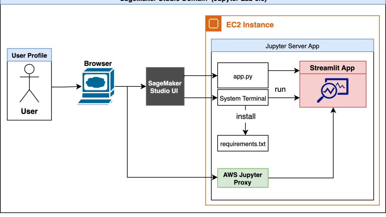
The following is the architecture diagram of our solution.

A user first accesses Studio through the browser. The Jupyter Server associated with the user profile runs inside the Studio Amazon Elastic Compute Cloud (Amazon EC2) instance. Inside the Studio EC2 instance exists the example code and dependencies list. The user can run the Streamlit app, app.py, in the system terminal. Studio runs the JupyterLab UI in a Jupyter Server, decoupled from notebook kernels. The Jupyter Server comes with a proxy and allows us to access our Streamlit app. Once the app is running, the user can initiate a separate session through the AWS Jupyter Proxy by adjusting the URL.
From a security aspect, the AWS Jupyter Proxy is extended by AWS authentication. As long as a user has access to the AWS account, Studio domain ID, and user profile, they can access the link.
Create Studio using JupyterLab 3.0
Studio with JupyterLab 3 must be installed for this solution to work. Older versions might not support features outlined in this post. For more information, refer to Amazon SageMaker Studio and SageMaker Notebook Instance now come with JupyterLab 3 notebooks to boost developer productivity. By default, Studio comes with JupyterLab 3. You should check the version and change it if running an older version. For more information, refer to JupyterLab Versioning.
You can set up Studio using the AWS Cloud Development Kit (AWS CDK); for more information, refer to Set up Amazon SageMaker Studio with Jupyter Lab 3 using the AWS CDK. Alternatively, you can use the SageMaker console to change the domain settings. Complete the following steps:
- On the SageMaker console, choose Domains in the navigation pane.
- Select your domain and choose Edit.

- For Default Jupyter Lab version, make sure the version is set to Jupyter Lab 3.0.

(Optional) Create a Shared Space
We can use the SageMaker console or the AWS CLI to add support for shared spaces to an existing Domain by following the steps in the docs or in this blog. Creating a shared space in AWS has the following benefits:
- Collaboration: A shared space allows multiple users or teams to collaborate on a project or set of resources, without having to duplicate data or infrastructure.
- Cost savings: Instead of each user or team creating and managing their own resources, a shared space can be more cost-effective, as resources can be pooled and shared across multiple users.
- Simplified management: With a shared space, administrators can manage resources centrally, rather than having to manage multiple instances of the same resources for each user or team.
- Improved scalability: A shared space can be more easily scaled up or down to meet changing demands, as resources can be allocated dynamically to meet the needs of different users or teams.
- Enhanced security: By centralizing resources in a shared space, security can be improved, as access controls and monitoring can be applied more easily and consistently.
Install dependencies and clone the example on Studio
Next, we launch Studio and open the system terminal. We use the SageMaker IDE to clone our example and the system terminal to launch our app. The code for this blog can be found in this GitHub repository. We start with cloning the repository:

Next, we open the System Terminal.

Once cloned, in the system terminal install dependencies to run our example code by running the following command. This will first pip install the dependences by running pip install --no-cache-dir -r requirements.txt. The no-cache-dir flag will disable the cache. Caching helps store the installation files (.whl) of the modules that you install through pip. It also stores the source files (.tar.gz) to avoid re-download when they haven’t expired. If there isn’t space on our hard drive or if we want to keep a Docker image as small as possible, we can use this flag so the command runs to completion with minimal memory usage. Next the script will install packages iproute and jq , which will be used in the following step.sh setup.sh
Run Streamlit Demo and Create Shareable Link
To verify all dependencies are successfully installed and to view the Amazon Rekognition demo, run the following command:
The port number hosting the app will be displayed.
Note that while developing, it might be helpful to automatically rerun the script when app.py is modified on disk. To do, so we can modify the runOnSave configuration option by adding the --server.runOnSave true flag to our command:
The following screenshot shows an example of what should be displayed on the terminal.

From the above example we see the port number, domain ID, and studio URL we are running our app on. Finally, we can see the URL we need to use to access our streamlit app. This script is modifying the Studio URL, replacing lab? with proxy/[PORT NUMBER]/ . The Rekognition Object Detection Demo will be displayed, as shown in the following screenshot.

Now that we have the Streamlit app working, we can share this URL with anyone who has access to this Studio domain ID and user profile. To make sharing these demos easier, we can check the status and list all running streamlit apps by running the following command: sh status.sh
We can use lifecycle scripts or shared spaces to extend this work. Instead of manually running the shell scripts and installing dependencies, use lifecycle scripts to streamline this process. To develop and extend this app with a team and share dashboards with peers, use shared spaces. By creating shared spaces in Studio, users can collaborate in the shared space to develop a Streamlit app in real time. All resources in a shared space are filtered and tagged, making it easier to focus on ML projects and manage costs. Refer to the following code to make your own applications in Studio.
Cleanup
Once we are done using the app, we want to free up the listening ports. To get all the processes running streamlit and free them up for use we can run our cleanup script: sh cleanup.sh
Conclusion
In this post, we showed an end-to-end example of hosting a Streamlit demo for an object detection task using Amazon Rekognition. We detailed the motivations for building quick web applications, security considerations, and setup required to run our own Streamlit app in Studio. Finally, we modified the URL pattern in our web browser to initiate a separate session through the AWS Jupyter Proxy.
This demo allows you to upload any image and visualize the outputs from Amazon Rekognition. The results are also processed, and you can download a CSV file with all the bounding boxes through the app. You can extend this work to annotate and label your own dataset, or modify the code to showcase your custom model!
About the Authors
 Dipika Khullar is an ML Engineer in the Amazon ML Solutions Lab. She helps customers integrate ML solutions to solve their business problems. Most recently, she has built training and inference pipelines for media customers and predictive models for marketing.
 Marcelo Aberle is an ML Engineer in the AWS AI organization. He is leading MLOps efforts at the Amazon ML Solutions Lab, helping customers design and implement scalable ML systems. His mission is to guide customers on their enterprise ML journey and accelerate their ML path to production.
 Yash Shah is a Science Manager in the Amazon ML Solutions Lab. He and his team of applied scientists and ML engineers work on a range of ML use cases from healthcare, sports, automotive, and manufacturing.
Secure Amazon SageMaker Studio presigned URLs Part 3: Multi-account private API access to Studio
Enterprise customers have multiple lines of businesses (LOBs) and groups and teams within them. These customers need to balance governance, security, and compliance against the need for machine learning (ML) teams to quickly access their data science environments in a secure manner. These enterprise customers that are starting to adopt AWS, expanding their footprint on AWS, or plannng to enhance an established AWS environment need to ensure they have a strong foundation for their cloud environment. One important aspect of this foundation is to organize their AWS environment following a multi-account strategy.
In the post Secure Amazon SageMaker Studio presigned URLs Part 2: Private API with JWT authentication, we demonstrated how to build a private API to generate Amazon SageMaker Studio presigned URLs that are only accessible by an authenticated end-user within the corporate network from a single account. In this post, we show how you can extend that architecture to multiple accounts to support multiple LOBs. We demonstrate how you can use Studio presigned URLs in a multi-account environment to secure and route access from different personas to their appropriate Studio domain. We explain the process and network flow, and how to easily scale this architecture to multiple accounts and Amazon SageMaker domains. The proposed solution also ensures that all network traffic stays within AWS’s private network and communication happens in a secure way.
Although we demonstrate using two different LOBs, each with a separate AWS account, this solution can scale to multiple LOBs. We also introduce a logical construct of a shared services account that plays a key role in governance, administration, and orchestration.
Solution overview
We can achieve communication between all LOBs’ SageMaker VPCs and the shared services account VPC using either VPC peering or AWS Transit Gateway. In this post, we use a transit gateway because it provides a simpler VPC-to-VPC communication mechanism over VPC peering when there are a large number of VPCs involved. We also use Amazon Route 53 forwarding rules in combination with inbound and outbound resolvers to resolve all DNS queries to the shared service account VPC endpoints. The networking architecture has been designed using the following patterns:
- Centralizing VPC endpoints with Transit Gateway
- Associating a transit gateway across accounts
- Privately access a central AWS service endpoint from multiple VPCs
Let’s look at the two main architecture components, the information flow and network flow, in more detail.
Information flow
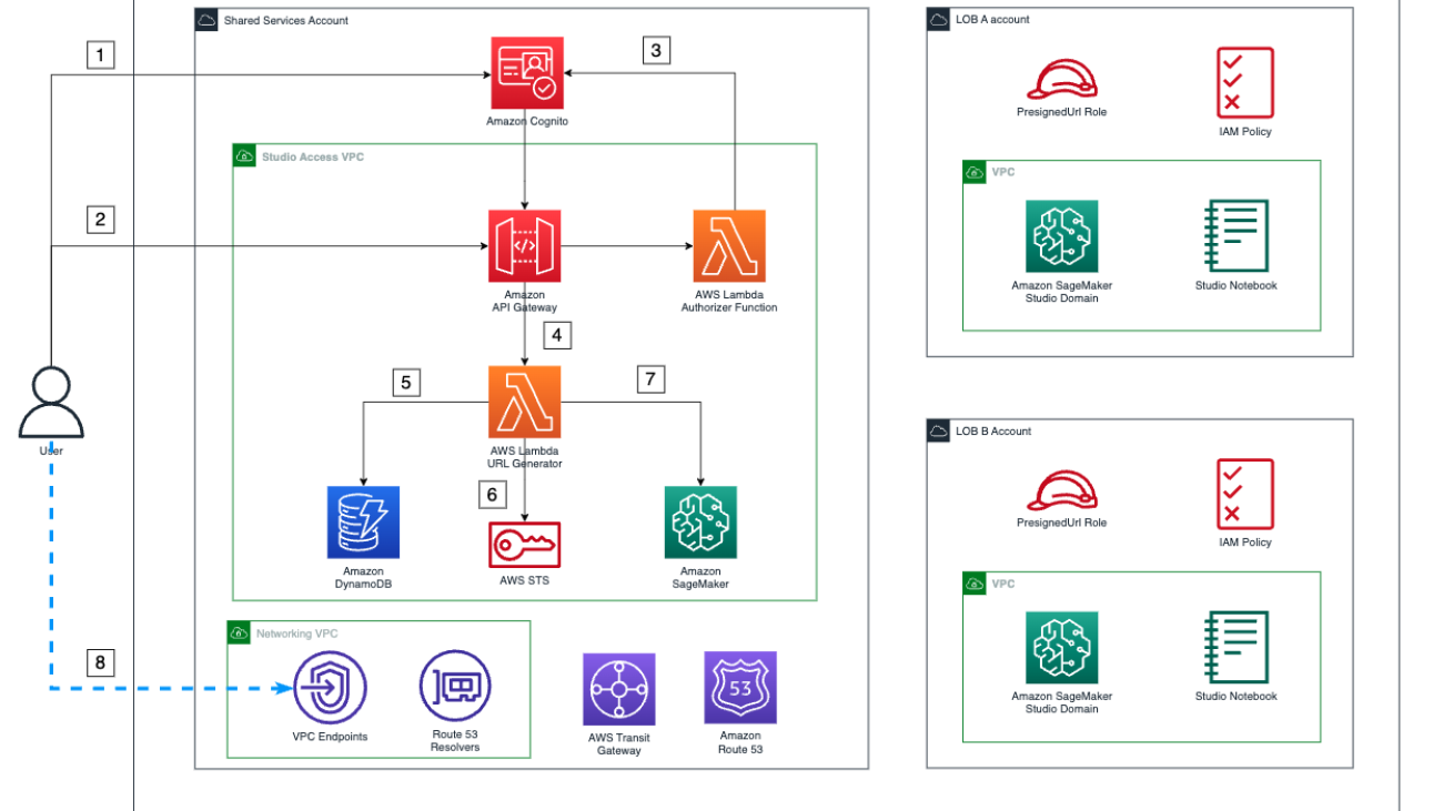
The following diagram illustrates the architecture of the information flow.

The workflow steps are as follows:
- The user authenticates with the Amazon Cognito user pool and receives a token to consume the Studio access API.
- The user calls the API to access Studio and includes the token in the request.
- When this API is invoked, the custom AWS Lambda authorizer is triggered to validate the token with the identity provider (IdP), and returns the proper permissions for the user.
- After the call is authorized, a Lambda function is triggered.
- This Lambda function uses the user’s name to retrieve their LOB name and the LOB account from the following Amazon DynamoDB tables that store these relationships:
- Users table – This table holds the relationship between users and their LOB.
- LOBs table – This table holds the relationship between the LOBs and the AWS account where the SageMaker domain for that LOB exists.
- With the account ID, the Lambda function assumes the PresignedUrlGenerator role in that account (each LOB account has a PresignedURLGenerator role that can only be assumed by the Lambda function in charge of generating the presigned URLs).
- Finally, the function invokes the SageMaker create-presigned-domain-url API call for that user in their LOB´s SageMaker domain.
- The presigned URL is returned to the end-user, who consumes it via the Studio VPC endpoint.
Steps 1–4 are covered in more detail in Part 2 of this series, where we explain how the custom Lambda authorizer works and takes care of the authorization process in the access API Gateway.
Network flow
All network traffic flows in a secure and private manner using AWS PrivateLink, as shown in the following diagram.

The steps are as follows:
- When the user calls the access API, it happens via the VPC endpoint for Amazon API Gateway in the networking VPC in the shared services account. This API is set as private, and has a policy that allows its consumption only via this VPC endpoint, as described in Part 2 of this series.
- All the authorization process happens privately between API Gateway, Lambda, and Amazon Cognito.
- After authorization is granted, API Gateway triggers the Lambda function in charge of generating the presigned URLs using AWS’s private network.
- Then, because the routing Lambda function lives in a VPC, all calls to different services happen through their respective VPC endpoints in the shared services account. The function performs the following actions:
- Retrieve the credentials to assume the role via the AWS Security Token Service (AWS STS) VPC endpoint in the networking account.
- Call DynamoDB to retrieve user and LOB information through the DynamoDB VPC endpoint.
- Call the SageMaker API to create a presigned URL for the user in their SageMaker domain through the SageMaker API VPC endpoint.
- The user finally consumes the presigned URL via the Studio VPC endpoint in the networking VPC in the shared services account, because this VPC endpoint has been specified during the creation of the presigned URL.
- All further communications between Studio and AWS services happen via Studio’s ENI inside the LOB account’s SageMaker VPC. For example, to allow SageMaker to call Amazon Elastic Container Registry (Amazon ECR), the Amazon ECR interface VPC endpoint can be provisioned in the shared services account VPC, and a forwarding rule is shared with the SageMaker accounts that need to consume it. This allows SageMaker queries to Amazon ECR to be resolved to this endpoint, and the Transit Gateway routing will do the rest.
Prerequisites
To represent a multi-account environment, we use one shared services account and two different LOBs:
- Shared services account – Where the VPC endpoints and the Studio access Gateway API live
- SageMaker account LOB A – The account for the SageMaker domain for LOB A
- SageMaker account LOB B – The account for the SageMaker domain for LOB B
For more information on how to create an AWS account, refer to How do I create and activate a new AWS account.
LOB accounts are logical entities that are business, department, or domain specific. We assume one account per logical entity. However, there will be different accounts per environment (development, test, production). For each environment, you typically have a separate shared services account (based on compliance requirements) to restrict the blast radius.
You can use the templates and instructions in the GitHub repository to set up the needed infrastructure. This repository is structured into folders for the different accounts and different parts of the solution.
Infrastructure setup
For large companies with many Studio domains, it’s also advisable to have a centralized endpoint architecture. This can result in cost savings as the architecture scales and more domains and accounts are created. The networking.yml template in the shared services account deploys the VPC endpoints and needed Route 53 resources, and the Transit Gateway infrastructure to scale out the proposed solution.
Detailed instructions of the deployment can be found in the README.md file in the GitHub repository. The full deployment includes the following resources:
- Two AWS CloudFormation templates in the shared services account: one for networking infrastructure and one for the AWS Serverless Application Model (AWS SAM) Studio access Gateway API
- One CloudFormation template for the infrastructure in the SageMaker account LOB A
- One CloudFormation template for the infrastructure of the SageMaker account LOB B
- Optionally, an on-premises simulator can be deployed in the shared services account to test the end-to-end deployment
After everything is deployed, navigate to the Transit Gateway console for each SageMaker account (LOB accounts) and confirm that the transit gateway has been correctly shared and the VPCs are associated with it.
Optionally, if any forwarding rules have been shared with the accounts, they can be associated with the SageMaker accounts’ VPC. The basic rules to make the centralized VPC endpoints solution work are automatically shared with the LOB Account during deployment. For more information about this approach, refer to Centralized access to VPC private endpoints.
Populate the data
Run the following script to populate the DynamoDB tables and Amazon Cognito user pool with the required information:
The script performs the required API calls using the AWS Command Line Interface (AWS CLI) and the previously configured parameters and profiles.
Amazon Cognito users
This step works the same as Part 2 of this series, but has to be performed for users in all LOBs and should match their user profile in SageMaker, regardless of which LOB they belong to. For this post, we have one user in a Studio domain in LOB A (user-lob-a) and one user in a Studio domain in LOB B (user-lob-b). The following table lists the users populated in the Amazon Cognito user pool.
| User | Password |
| user-lob-a | UserLobA1! |
| user-lob-b | UserLobB1! |
Note that these passwords have been configured for demo purposes.
DynamoDB tables
The access application uses two DynamoDB tables to direct requests from the different users to their LOB’s Studio domain.
The users table holds the relationship between users and their LOB.
| Primary Key | LOB |
| user-lob-a | lob-a |
| user-lob-b | lob-b |
The LOB table holds the relationship between the LOB and the AWS account where the SageMaker domain for that LOB exists.
| LOB | ACCOUNT_ID |
| lob-a | <YOUR_LOB_A_ACCOUNT_ID> |
| lob-b | <YOUR_LOB_B_ACCOUNT_ID> |

Note that these user names must be consistent across the Studio user profiles and the names of the users we previously added to the Amazon Cognito user pool.
Test the deployment
At this point, we can test the deployment going to API Gateway and check what the API responds for any of the users. We get a presigned URL in the response; however, consuming that URL in the browser will give an auth token error.


For this demo, we have set up a simulated on-premises environment with a bastion host and a Windows application. We install Firefox in the Windows instance and use the dev tools to add authorization headers to our requests and test the solution. More detailed information on how to set up the on-premises simulated environment is available in the associated GitHub repository.
The following diagram shows our test architecture.

We have two users, one for LOB A (User A) and another one for LOB B (User B), and we show how the Studio domain changes just by changing the authorization key retrieved from Amazon Cognito when logging in as User A and User B.
Complete the following steps to test the deployment:
- Retrieve the session token for User A, as shown in Part 2 of the series and also in the instructions in the GitHub repository.
We use the following example command to get the user credentials from Amazon Cognito:
- For this demo, we use a simulated Windows on-premises application. To connect to the Windows instance, you can follow the same approach specified in Secure access to Amazon SageMaker Studio with AWS SSO and a SAML application.
- Firefox should be installed in the instance. If not, once in the instance, we can install Firefox.
- Open Firefox and try to access the API of Studio with either
user-lob-aoruser-lob-bas the API path parameter.
You get a not authorized message.

- Open the developer tools of Firefox and on the Network tab, choose (right-click) the previous API call, and choose Edit and Resend.

- Here we add the token as an authorization header in the Firefox developer tools and make the request to the Studio access Gateway API again.

This time, we see in the developer tools that the URL is returned along with a 302 redirect.

- Although the redirect won´t work when using the developer tools, you can still choose it to access the LOB SageMaker domain for that user.

- Repeat for User B with its corresponding token and check that they get redirected to a different Studio domain.
If you perform these steps correctly, you can access both domains at the same time.
In our on-premises Windows application, we can have both domains consumed via the Studio VPC endpoint through our VPC peering connection.

Let’s explore some other testing scenarios.
If you edit the API again and change the path to the opposite LOB, when resending, we get an error in the API response: a forbidden response from API Gateway.

Trying to take the returned URL for the correct user and consume it in your laptop´s browser will also fail, because it won’t be consumed via the internal Studio VPC endpoint. This is the same error we saw when testing with API Gateway. It returns an “Auth token containing insufficient permissions” error.

Taking too long to consume the presigned URL will result in an “Invalid or Expired Auth Token” error.

Scale domains
Whenever a new SageMaker domain is added, you must complete the following networking and access steps:
- Share the transit gateway with the new account using AWS Resource Access Manager (AWS RAM).
- Attach the VPC to the transit gateway in the LOB account (this is done in AWS CloudFormation).
In our scenario, the transit gateway was set with automatic association to the default route table and automatic propagation enabled. In a real-world use case, you may need to complete three additional steps:
- In the shared services account, associate the attached Studio VPC to the respective Transit Gateway route table for SageMaker domains.
- Propagate the associated VPC routes to Transit Gateway.
- Lastly, add the account ID along with the LOB name to the LOBs’ DynamoDB table.
Clean up
Complete the following steps to clean up your resources:
- Delete the VPC peering connection.
- Remove the associated VPCs from the private hosted zones.
- Delete the on-premises simulator template from the shared services account.
- Delete the Studio CloudFormation templates from the SageMaker accounts.
- Delete the access CloudFormation template from the shared services account.
- Delete the networking CloudFormation template from the shared services account.
Conclusion
In this post, we walked through how you can set up multi-account private API access to Studio. We explained how the networking and application flows happen as well as how you can easily scale this architecture for multiple accounts and SageMaker domains. Head over to the GitHub repository to begin your journey. We’d love to hear your feedback!
About the Authors
 Neelam Koshiya is an Enterprise Solutions Architect at AWS. Her current focus is helping enterprise customers with their cloud adoption journey for strategic business outcomes. In her spare time, she enjoys reading and being outdoors.
 Alberto Menendez is an Associate DevOps Consultant in Professional Services at AWS. He helps accelerate customers´ journeys to the cloud. In his free time, he enjoys playing sports, especially basketball and padel, spending time with family and friends, and learning about technology.
 Rajesh Ramchander is a Senior Data & ML Engineer in Professional Services at AWS. He helps customers migrate big data and AL/ML workloads to AWS.
 Ram Vittal is a machine learning solutions architect at AWS. He has over 20 years of experience architecting and building distributed, hybrid, and cloud applications. He is passionate about building secure and scalable AI/ML and big data solutions to help enterprise customers with their cloud adoption and optimization journey to improve their business outcomes. In his spare time, he enjoys tennis and photography.

Run secure processing jobs using PySpark in Amazon SageMaker Pipelines
Amazon SageMaker Studio can help you build, train, debug, deploy, and monitor your models and manage your machine learning (ML) workflows. Amazon SageMaker Pipelines enables you to build a secure, scalable, and flexible MLOps platform within Studio.
In this post, we explain how to run PySpark processing jobs within a pipeline. This enables anyone that wants to train a model using Pipelines to also preprocess training data, postprocess inference data, or evaluate models using PySpark. This capability is especially relevant when you need to process large-scale data. In addition, we showcase how to optimize your PySpark steps using configurations and Spark UI logs.
Pipelines is an Amazon SageMaker tool for building and managing end-to-end ML pipelines. It’s a fully managed on-demand service, integrated with SageMaker and other AWS services, and therefore creates and manages resources for you. This ensures that instances are only provisioned and used when running the pipelines. Furthermore, Pipelines is supported by the SageMaker Python SDK, letting you track your data lineage and reuse steps by caching them to ease development time and cost. A SageMaker pipeline can use processing steps to process data or perform model evaluation.
When processing large-scale data, data scientists and ML engineers often use PySpark, an interface for Apache Spark in Python. SageMaker provides prebuilt Docker images that include PySpark and other dependencies needed to run distributed data processing jobs, including data transformations and feature engineering using the Spark framework. Although those images allow you to quickly start using PySpark in processing jobs, large-scale data processing often requires specific Spark configurations in order to optimize the distributed computing of the cluster created by SageMaker.
In our example, we create a SageMaker pipeline running a single processing step. For more information about what other steps you can add to a pipeline, refer to Pipeline Steps.
SageMaker Processing library
SageMaker Processing can run with specific frameworks (for example, SKlearnProcessor, PySparkProcessor, or Hugging Face). Independent of the framework used, each ProcessingStep requires the following:
- Step name – The name to be used for your SageMaker pipeline step
- Step arguments – The arguments for your
ProcessingStep
Additionally, you can provide the following:
- The configuration for your step cache in order to avoid unnecessary runs of your step in a SageMaker pipeline
- A list of step names, step instances, or step collection instances that the
ProcessingStepdepends on - The display name of the
ProcessingStep - A description of the
ProcessingStep - Property files
- Retry policies
The arguments are handed over to the ProcessingStep. You can use the sagemaker.spark.PySparkProcessor or sagemaker.spark.SparkJarProcessor class to run your Spark application inside of a processing job.
Each processor comes with its own needs, depending on the framework. This is best illustrated using the PySparkProcessor, where you can pass additional information to optimize the ProcessingStep further, for instance via the configuration parameter when running your job.
Run SageMaker Processing jobs in a secure environment
It’s best practice to create a private Amazon VPC and configure it so that your jobs aren’t accessible over the public internet. SageMaker Processing jobs allow you to specify the private subnets and security groups in your VPC as well as enable network isolation and inter-container traffic encryption using the NetworkConfig.VpcConfig request parameter of the CreateProcessingJob API. We provide examples of this configuration using the SageMaker SDK in the next section.
PySpark ProcessingStep within SageMaker Pipelines
For this example, we assume that you have Studio deployed in a secure environment already available, including VPC, VPC endpoints, security groups, AWS Identity and Access Management (IAM) roles, and AWS Key Management Service (AWS KMS) keys. We also assume that you have two buckets: one for artifacts like code and logs, and one for your data. The basic_infra.yaml file provides example AWS CloudFormation code to provision the necessary prerequisite infrastructure. The example code and deployment guide is also available on GitHub.
As an example, we set up a pipeline containing a single ProcessingStep in which we’re simply reading and writing the abalone dataset using Spark. The code samples show you how to set up and configure the ProcessingStep.
We define parameters for the pipeline (name, role, buckets, and so on) and step-specific settings (instance type and count, framework version, and so on). In this example, we use a secure setup and also define subnets, security groups, and the inter-container traffic encryption. For this example, you need a pipeline execution role with SageMaker full access and a VPC. See the following code:
{
	"pipeline_name": "ProcessingPipeline",
	"trial": "test-blog-post",
	"pipeline_role": "arn:aws:iam::<ACCOUNT_NUMBER>:role/<PIPELINE_EXECUTION_ROLE_NAME>",
	"network_subnet_ids": [
		"subnet-<SUBNET_ID>",
		"subnet-<SUBNET_ID>"
	],
	"network_security_group_ids": [
		"sg-<SG_ID>"
	],
	"pyspark_process_volume_kms": "arn:aws:kms:<REGION_NAME>:<ACCOUNT_NUMBER>:key/<KMS_KEY_ID>",
	"pyspark_process_output_kms": "arn:aws:kms:<REGION_NAME>:<ACCOUNT_NUMBER>:key/<KMS_KEY_ID>",
	"pyspark_helper_code": "s3://<INFRA_S3_BUCKET>/src/helper/data_utils.py",
	"spark_config_file": "s3://<INFRA_S3_BUCKET>/src/spark_configuration/configuration.json",
	"pyspark_process_code": "s3://<INFRA_S3_BUCKET>/src/processing/process_pyspark.py",
	"process_spark_ui_log_output": "s3://<DATA_S3_BUCKET>/spark_ui_logs/{}",
	"pyspark_framework_version": "2.4",
	"pyspark_process_name": "pyspark-processing",
	"pyspark_process_data_input": "s3a://<DATA_S3_BUCKET>/data_input/abalone_data.csv",
	"pyspark_process_data_output": "s3a://<DATA_S3_BUCKET>/pyspark/data_output",
	"pyspark_process_instance_type": "ml.m5.4xlarge",
	"pyspark_process_instance_count": 6,
	"tags": {
		"Project": "tag-for-project",
		"Owner": "tag-for-owner"
	}
}
To demonstrate, the following code example runs a PySpark script on SageMaker Processing within a pipeline by using the PySparkProcessor:
# import code requirements
# standard libraries import
import logging
import json

# sagemaker model import
import sagemaker
from sagemaker.workflow.pipeline import Pipeline
from sagemaker.workflow.pipeline_experiment_config import PipelineExperimentConfig
from sagemaker.workflow.steps import CacheConfig
from sagemaker.processing import ProcessingInput
from sagemaker.workflow.steps import ProcessingStep
from sagemaker.workflow.pipeline_context import PipelineSession
from sagemaker.spark.processing import PySparkProcessor

from helpers.infra.networking.networking import get_network_configuration
from helpers.infra.tags.tags import get_tags_input
from helpers.pipeline_utils import get_pipeline_config

def create_pipeline(pipeline_params, logger):
    """
    Args:
        pipeline_params (ml_pipeline.params.pipeline_params.py.Params): pipeline parameters
        logger (logger): logger
    Returns:
        ()
    """
    # Create SageMaker Session
    sagemaker_session = PipelineSession()

    # Get Tags
    tags_input = get_tags_input(pipeline_params["tags"])

    # get network configuration
    network_config = get_network_configuration(
        subnets=pipeline_params["network_subnet_ids"],
        security_group_ids=pipeline_params["network_security_group_ids"]
    )

    # Get Pipeline Configurations
    pipeline_config = get_pipeline_config(pipeline_params)

    # setting processing cache obj
    logger.info("Setting " + pipeline_params["pyspark_process_name"] + " cache configuration 3 to 30 days")
    cache_config = CacheConfig(enable_caching=True, expire_after="p30d")

    # Create PySpark Processing Step
    logger.info("Creating " + pipeline_params["pyspark_process_name"] + " processor")

    # setting up spark processor
    processing_pyspark_processor = PySparkProcessor(
        base_job_name=pipeline_params["pyspark_process_name"],
        framework_version=pipeline_params["pyspark_framework_version"],
        role=pipeline_params["pipeline_role"],
        instance_count=pipeline_params["pyspark_process_instance_count"],
        instance_type=pipeline_params["pyspark_process_instance_type"],
        volume_kms_key=pipeline_params["pyspark_process_volume_kms"],
        output_kms_key=pipeline_params["pyspark_process_output_kms"],
        network_config=network_config,
        tags=tags_input,
        sagemaker_session=sagemaker_session
    )

    # setting up arguments
    run_ags = processing_pyspark_processor.run(
        submit_app=pipeline_params["pyspark_process_code"],
        submit_py_files=[pipeline_params["pyspark_helper_code"]],
        arguments=[
        # processing input arguments. To add new arguments to this list you need to provide two entrances:
        # 1st is the argument name preceded by "--" and the 2nd is the argument value
        # setting up processing arguments
            "--input_table", pipeline_params["pyspark_process_data_input"],
            "--output_table", pipeline_params["pyspark_process_data_output"]
        ],
        spark_event_logs_s3_uri=pipeline_params["process_spark_ui_log_output"].format(pipeline_params["trial"]),
        inputs = [
            ProcessingInput(
                source=pipeline_params["spark_config_file"],
                destination="/opt/ml/processing/input/conf",
                s3_data_type="S3Prefix",
                s3_input_mode="File",
                s3_data_distribution_type="FullyReplicated",
                s3_compression_type="None"
            )
        ],
    )

    # create step
    pyspark_processing_step = ProcessingStep(
        name=pipeline_params["pyspark_process_name"],
        step_args=run_ags,
        cache_config=cache_config,
    )

    # Create Pipeline
    pipeline = Pipeline(
        name=pipeline_params["pipeline_name"],
        steps=[
            pyspark_processing_step
        ],
        pipeline_experiment_config=PipelineExperimentConfig(
            pipeline_params["pipeline_name"],
            pipeline_config["trial"]
        ),
        sagemaker_session=sagemaker_session
    )
    pipeline.upsert(
        role_arn=pipeline_params["pipeline_role"],
        description="Example pipeline",
        tags=tags_input
    )
    return pipeline


def main():
    # set up logging
    logger = logging.getLogger(__name__)
    logger.setLevel(logging.INFO)
    logger.info("Get Pipeline Parameter")

    with open("ml_pipeline/params/pipeline_params.json", "r") as f:
        pipeline_params = json.load(f)
    print(pipeline_params)

    logger.info("Create Pipeline")
    pipeline = create_pipeline(pipeline_params, logger=logger)
    logger.info("Execute Pipeline")
    execution = pipeline.start()
    return execution


if __name__ == "__main__":
    main()
As shown in the preceding code, we’re overwriting the default Spark configurations by providing configuration.json as a ProcessingInput. We use a configuration.json file that was saved in Amazon Simple Storage Service (Amazon S3) with the following settings:
[
    {
        "Classification":"spark-defaults",
        "Properties":{
            "spark.executor.memory":"10g",
            "spark.executor.memoryOverhead":"5g",
            "spark.driver.memory":"10g",
            "spark.driver.memoryOverhead":"10g",
            "spark.driver.maxResultSize":"10g",
            "spark.executor.cores":5,
            "spark.executor.instances":5,
            "spark.yarn.maxAppAttempts":1
            "spark.hadoop.fs.s3a.endpoint":"s3.<region>.amazonaws.com",
            "spark.sql.parquet.fs.optimized.comitter.optimization-enabled":true
        }
    }
]
We can update the default Spark configuration either by passing the file as a ProcessingInput or by using the configuration argument when running the run() function.
The Spark configuration is dependent on other options, like the instance type and instance count chosen for the processing job. The first consideration is the number of instances, the vCPU cores that each of those instances have, and the instance memory. You can use Spark UIs or CloudWatch instance metrics and logs to calibrate these values over multiple run iterations.
In addition, the executor and driver settings can be optimized even further. For an example of how to calculate these, refer to Best practices for successfully managing memory for Apache Spark applications on Amazon EMR.
Next, for driver and executor settings, we recommend investigating the committer settings to improve performance when writing to Amazon S3. In our case, we’re writing Parquet files to Amazon S3 and setting “spark.sql.parquet.fs.optimized.comitter.optimization-enabled” to true.
If needed for a connection to Amazon S3, a regional endpoint “spark.hadoop.fs.s3a.endpoint” can be specified within the configurations file.
In this example pipeline, the PySpark script spark_process.py (as shown in the following code) loads a CSV file from Amazon S3 into a Spark data frame, and saves the data as Parquet back to Amazon S3.
Note that our example configuration is not proportionate to the workload because reading and writing the abalone dataset could be done on default settings on one instance. The configurations we mentioned should be defined based on your specific needs.
# import requirements
import argparse
import logging
import sys
import os
import pandas as pd

# spark imports
from pyspark.sql import SparkSession
from pyspark.sql.functions import (udf, col)
from pyspark.sql.types import StringType, StructField, StructType, FloatType

from data_utils import(
    spark_read_parquet,
    Unbuffered
)

sys.stdout = Unbuffered(sys.stdout)

# Define custom handler
logger = logging.getLogger(__name__)
handler = logging.StreamHandler(sys.stdout)
handler.setFormatter(logging.Formatter("%(asctime)s %(message)s"))
logger.addHandler(handler)
logger.setLevel(logging.INFO)

def main(data_path):

    spark = SparkSession.builder.appName("PySparkJob").getOrCreate()
    spark.sparkContext.setLogLevel("ERROR")

    schema = StructType(
        [
            StructField("sex", StringType(), True),
            StructField("length", FloatType(), True),
            StructField("diameter", FloatType(), True),
            StructField("height", FloatType(), True),
            StructField("whole_weight", FloatType(), True),
            StructField("shucked_weight", FloatType(), True),
            StructField("viscera_weight", FloatType(), True),
            StructField("rings", FloatType(), True),
        ]
    )

    df = spark.read.csv(data_path, header=False, schema=schema)
    return df.select("sex", "length", "diameter", "rings")

if __name__ == "__main__":
    logger.info(f"===============================================================")
    logger.info(f"================= Starting pyspark-processing =================")
    parser = argparse.ArgumentParser(description="app inputs")
    parser.add_argument("--input_table", type=str, help="path to the channel data")
    parser.add_argument("--output_table", type=str, help="path to the output data")
    args = parser.parse_args()

    df = main(args.input_table)

    logger.info("Writing transformed data")
    df.write.csv(os.path.join(args.output_table, "transformed.csv"), header=True, mode="overwrite")

    # save data
    df.coalesce(10).write.mode("overwrite").parquet(args.output_table)

    logger.info(f"================== Ending pyspark-processing ==================")
    logger.info(f"===============================================================")
To dive into optimizing Spark processing jobs, you can use the CloudWatch logs as well as the Spark UI. You can create the Spark UI by running a Processing job on a SageMaker notebook instance. You can view the Spark UI for the Processing jobs running within a pipeline by running the history server within a SageMaker notebook instance if the Spark UI logs were saved within the same Amazon S3 location.
Clean up
If you followed the tutorial, it’s good practice to delete resources that are no longer used to stop incurring charges. Make sure to delete the CloudFormation stack that you used to create your resources. This will delete the stack created as well as the resources it created.
Conclusion
In this post, we showed how to run a secure SageMaker Processing job using PySpark within SageMaker Pipelines. We also demonstrated how to optimize PySpark using Spark configurations and set up your Processing job to run in a secure networking configuration.
As a next step, explore how to automate the entire model lifecycle and how customers built secure and scalable MLOps platforms using SageMaker services.
About the Authors
 Maren Suilmann is a Data Scientist at AWS Professional Services. She works with customers across industries unveiling the power of AI/ML to achieve their business outcomes. Maren has been with AWS since November 2019. In her spare time, she enjoys kickboxing, hiking to great views, and board game nights.
 Maira Ladeira Tanke is an ML Specialist at AWS. With a background in data science, she has 9 years of experience architecting and building ML applications with customers across industries. As a technical lead, she helps customers accelerate their achievement of business value through emerging technologies and innovative solutions. In her free time, Maira enjoys traveling and spending time with her family someplace warm.
 Pauline Ting is Data Scientist in the AWS Professional Services team. She supports customers in achieving and accelerating their business outcome by developing AI/ML solutions. In her spare time, Pauline enjoys traveling, surfing, and trying new dessert places.
 Donald Fossouo is a Sr Data Architect in the AWS Professional Services team, mostly working with Global Finance Service. He engages with customers to create innovative solutions that address customer business problems and accelerate the adoption of AWS services. In his spare time, Donald enjoys reading, running, and traveling.

Create your RStudio on Amazon SageMaker licensed or trial environment in three easy steps
RStudio on Amazon SageMaker is the first fully managed cloud-based Posit Workbench (formerly known as RStudio Workbench). RStudio on Amazon SageMaker removes the need for you to manage the underlying Posit Workbench infrastructure, so your teams can concentrate on producing value for your business. You can quickly launch the familiar RStudio integrated development environment (IDE) and scale up and down the underlying compute resources without interrupting your work, making it easy to build machine learning (ML) and analytics solutions in R at scale.
Setting up a new Amazon SageMaker Studio domain with RStudio support or adding RStudio to an existing domain is now easier, thanks to the service integration with AWS Marketplace and AWS License Manager. You can now acquire your new Posit Workbench license or request a trial directly from AWS Marketplace and set up your environment using the AWS Management Console. In this post, we walk you through this process in three straightforward steps:
- Acquire a Posit Workbench license or request a time-bound trial in AWS Marketplace.
- Create a license grant in License Manager for your AWS account.
- Provision a new Studio domain with RStudio or add RStudio to your existing domain.
Prerequisites
Before beginning this walkthrough, make sure you have the following prerequisites:
- An AWS account that will host your Amazon SageMaker domain. If you’re setting up a production environment, it’s recommended to have a dedicated account for your SageMaker domain and manage your licenses in a shared services account. For more information on how to organize your multi-account environment, refer to Organizing Your AWS Environment Using Multiple Accounts.
- An AWS Identity and Access Management (IAM) role with access to the following services (for details on the specific permissions required, refer to Create an Amazon SageMaker Domain with RStudio using the AWS CLI):
- AWS Marketplace
- License Manager
Step 1: Acquire your Posit Workbench license
To acquire your Posit Workbench license, complete the following steps:
- Log in to your AWS account and navigate to the AWS Marketplace console.
- In the navigation pane, choose Discover Products.
- Search for Posit, then choose Posit Workbench and choose Continue to Subscribe.

Fig 1: Posit Workbench product page on AWS marketplace
- Specify your settings for Contract duration, Renewal Settings, and Contract options, then choose Create Contract.

Fig 2: Posit Workbench product agreement page on AWS marketplace
You will see a message stating your request is being processed. This step will take a few minutes to complete.

Fig 3: AWS Marketplace manage subscriptions page
After few minutes, you see the RStudio Workbench product under your subscriptions.
Request a trial license
If you want to create a test environment or a proof of concept, you can use the Posit Workbench product page to request a trial license. Complete the following steps:
- Locate the evaluation request form link on the Overview tab in AWS Marketplace.

Fig 4: Contact from link in Posit Workbench product page
- Fill out the contact form and make sure you include your AWS account ID in the How we can help? prompt.
This is very important because that will allow you to get the trial license private offer directly to your email without any additional back and forth.
You will receive an email with a link to a $0 limited-time private offer that you can open while logged in to your AWS account. After you accept the offer, you will be able to follow the next steps to activate your license grant.
Step 2: Manage your license grant in License Manager
To activate your license grant, complete the following steps:
- Navigate to the License Manager console to view the Posit Workbench license.
- If you’re using License Manager for the first time, you need to grant permission to use License Manager by selecting I grant AWS License Manager the required permissions and choosing Grant permissions.
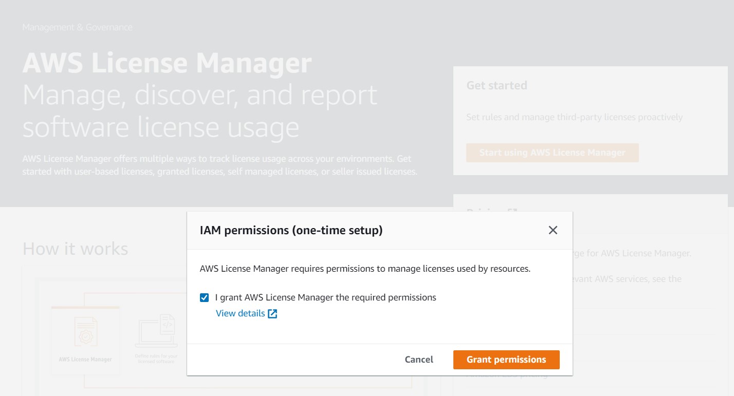
Fig 5: AWS License Manager one-time setup page for IAM Permissions
- Choose Granted licenses in the navigation pane.
You can see two entitlements related to Posit Workbench: one for AWS Marketplace usage and the other for named users. In order to be able to use your license and create a Studio domain with RStudio support, you need to accept the license.
- On the Granted licenses page, select the license grant with RStudio Workbench as the product name and choose View.
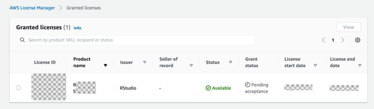
Fig 6: AWS License Manager console with Granted licenses
- On the license detail page, choose Accept & activate license.
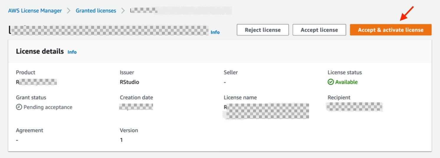
Fig 7: AWS License Manager console with License details
If you have a single account and want to create your Studio domain in the same account you’re managing your license, you can jump to Step 11. However, it’s an AWS recommended best practice to use a multi-account AWS environment where you have a dedicated shared services account to manage your licenses. If that’s the case, you need to create a license grant for the AWS account where you will create the Studio domain with RStudio.
- In the navigation pane, choose Granted licenses, then choose the license ID to open the license details page.
- In the Grants section, choose Create grant.
- Enter a name and AWS account ID of the grant recipient (the AWS account where you will create your RStudio-enabled Studio domain).
- Choose Create grant.

Fig 8: Create grant page in AWS License Manager console
- Log in to the AWS account where you will set up your RStudio on Amazon SageMaker domain and navigate to the License Manager console to accept and activate the granted license that appears as Pending acceptance.
The status changes to Active when you accept the grant or Rejected otherwise.
- Choose the license ID to see the details of the license.
- Choose Accept & activate license.

Fig 9: Amazon License Manager console with license status available
The license status changes to Available.
- To finalize, choose Activate license.

Fig 10: Amazon License Manager console with active license status
Now that you have accepted your Posit Workbench license, you’re ready to create your RStudio on Amazon SageMaker domain. Your license can be consumed by RStudio on Amazon SageMaker in any AWS Region that supports the feature.
Prerequisites to create a SageMaker domain
RStudio on Amazon SageMaker requires an IAM execution role that has permissions to License Manager and Amazon CloudWatch. For instructions, refer to Create DomainExecution role.
You can also use the following AWS CloudFormation stack template that creates the required IAM execution role in your account. Complete the following steps:
- Choose Launch Stack:
![]()
The link takes you to the us-east-1 Region, but you can change to your preferred Region. IAM roles are global resources, so you can access the role in any Region.
- In the Specify template section, choose Next.
- In the Specify stack details section, for Stack name, enter a name and choose Next.
- In the Configure stack options section, choose Next.
- In the Review section, select I acknowledge that AWS CloudFormation might create IAM resources and choose Create stack.
- When the stack status changes to
CREATE_COMPLETE, go to the Resources tab to find the IAM role you created.
Step 3: Create a Studio domain with RStudio
You can configure RStudio on Amazon SageMaker as part of a multi-step SageMaker domain creation process on the console. You can also perform the steps using the AWS Command Line Interface (AWS CLI) following the instructions on Create an Amazon SageMaker Domain with RStudio using the AWS CLI. To create your domain on the console, complete the following steps:
- On the SageMaker console, on the Setup SageMaker Domain page, choose Standard setup , and choose Configure.

Fig 11: Amazon SageMaker domain creation
- In Step 1 of the Standard setup, you will need to provide:
- Your domain name.
- Your chosen authentication method (IAM or AWS Identity Center)
- Your domain execution role (see the pre-requisites section above).
- Your network and storage selection.
- In Step 2 you will provide configuration of your Studio Jupyter Lab environment (you can keep the default values and proceed).
- In Step 3, Studio automatically detects your RStudio Workbench license after it’s added and accepted in License Manager, as seen below.

Fig12: Amazon SageMaker domain creation – general settings
You can choose the instance type for the RStudio server that is going to be shared by all users in your domain. ml.t3.medium is recommended for Domains with low UI use and is free to use. For more information about how to choose an instance type, see RStudioServerPro instance type page. Note that this is not the instance where your R sessions run their analysis and ML code.
The domain creation takes a couple of minutes. When it’s complete, we can add users for data scientists to access RStudio on SageMaker.
Add RStudio support to an existing Studio domain
If you already have a SageMaker domain, you can add RStudio support by using the update-domain API call from the AWS CLI. Complete the following steps:
- Delete all apps in your SageMaker domain. This is necessary because adding RStudio will update all your existing user profile security groups.
- Obtain a list of all existing apps by running the following command:
- Then delete every app by running the following command:
- Activate RStudio by updating your domain. Depending on the type of networking you have set up your domain with, you will choose between the following code examples:
- If your domain is in
VPCOnlymode: - If your domain is in
PublicInternetOnlymode:
- If your domain is in
Important: If you have modified the security groups for existing user profiles in your domain, you have to make an additional update to make sure you don’t run into the maximum number of security groups per Elastic Network Interface limit. For more information, refer to Add RStudio support to an existing Domain.
- You can now start adding new user profiles to your domain with RStudio support (by default, they will have access to RStudio). You can also add RStudio access to pre-existing user profiles. This is necessary because, by default, pre-existing user profiles in the domain are not granted access to RStudio on SageMaker.
- Run the following command to add RStudio access to existing user profiles:
Create a Studio domain user profile
Creating a user in your Studio domain allows access to both Studio and RStudio on SageMaker. You can configure both on the SageMaker console. If you prefer to use the AWS CLI to set up a user, refer to Manage users. To enable RStudio for a user via the console, complete the following steps:
- On the Domain details page, choose Add user.
- For Name, enter a user name.
- For Default execution role, create the user profile’s execution role.
- Choose Next.

Fig 13: Amazon SageMaker Add user– General Settings tab
- Next, you can configure the access to SageMaker project templates and JumpStart. You can keep it default even though we don’t use this feature in this post; you can always edit it later.
- Choose Next to proceed.
- For License Authorization, Studio automatically detects and adds RStudio Workbench licenses to the domain for you to choose from:
-
- RStudio Admin – Has access to the RStudio IDE and RStudio administrative dashboard
- RStudio User – Has access to the RStudio IDE
- Unauthorized – Doesn’t have access to the RStudio IDE
Note that all options grant access to Studio.
- Choose either RStudio Admin or RStudio User and choose Next to proceed.
- Choose Submit.
The user profile creation takes less than a minute.

Fig 14: Amazon SageMaker Add user – RStudio setting tab
- To open RStudio on SageMaker, on the Launch app menu in the user list, choose RStudio.

Fig 15: Amazon SageMaker Domain users
You will see the RStudio Workbench home page and a list of sessions, projects, and published content.
- To create a new session, choose New Session.
- Choose a desired instance on the Instance Type menu and choose Start Session.

Fig 16: Creating a new RStudio session in RStudio workbench
When you launch your RStudio session, the Base R image serves as the basis of your instance. This Docker image includes R v4.0, AWS tools such as awscli, sagemaker, and boto3 Python packages, and the reticulate package for the interoperability between Python and R.

Fig 17: RStudio Workbench session
Clean up
As part of this walkthrough, you provisioned a SageMaker domain, user profiles, and RStudio session. To delete these resources, refer to Delete an Amazon SageMaker Domain.
Conclusion
In this post, we showed how you can easily set up your RStudio on Amazon SageMaker environment in three straightforward steps. You can now either acquire a new paid Posit Workbench license or request a trial directly from AWS Marketplace and quickly import your license using License Manager. We also showed you how, after you accept the license grant, Studio automatically detects your new license and allows you to create a Studio domain with Posit Workbench support. We encourage you to try out RStudio on Amazon SageMaker today by following these steps and give us your feedback in the comments section!
About the Authors
 Venkata Kampana is a Senior Solutions Architect in the AWS Health and Human Services team and is based in Sacramento, CA. In that role, he helps public sector customers achieve their mission objectives with well-architected solutions on AWS.
 Eric Peña is a Senior Technical Product Manager in the AWS Artificial Intelligence Platforms team, working on Amazon SageMaker Interactive Machine Learning. He currently focuses on IDE integrations on SageMaker Studio. He holds an MBA degree from MIT Sloan and outside of work enjoys playing basketball and football.
Amazon and University of Texas at Austin launch Science Hub
The collaboration supports education, community outreach, and the application of academic research to video streaming and robotics.Read More

Ask a Techspert: What is generative AI?
 A Google AI expert answers common questions about generative AI, large language models, machine learning and more.Read More
Announcing OpenAI’s Bug Bounty Program
This initiative is essential to our commitment to develop safe and advanced AI. As we create technology and services that are secure, reliable, and trustworthy, we need your help.OpenAI Blog