Dataset of images collected in an industrial setting features more than 190,000 objects, orders of magnitude more than previous datasets.Read More
Inpaint images with Stable Diffusion using Amazon SageMaker JumpStart
In November 2022, we announced that AWS customers can generate images from text with Stable Diffusion models using Amazon SageMaker JumpStart. Today, we are excited to introduce a new feature that enables users to inpaint images with Stable Diffusion models. Inpainting refers to the process of replacing a portion of an image with another image based on a textual prompt. By providing the original image, a mask image that outlines the portion to be replaced, and a textual prompt, the Stable Diffusion model can produce a new image that replaces the masked area with the object, subject, or environment described in the textual prompt.
You can use inpainting for restoring degraded images or creating new images with novel subjects or styles in certain sections. Within the realm of architectural design, Stable Diffusion inpainting can be applied to repair incomplete or damaged areas of building blueprints, providing precise information for construction crews. In the case of clinical MRI imaging, the patient’s head must be restrained, which may lead to subpar results due to the cropping artifact causing data loss or reduced diagnostic accuracy. Image inpainting can effectively help mitigate these suboptimal outcomes.
In this post, we present a comprehensive guide on deploying and running inference using the Stable Diffusion inpainting model in two methods: through JumpStart’s user interface (UI) in Amazon SageMaker Studio, and programmatically through JumpStart APIs available in the SageMaker Python SDK.
Solution overview
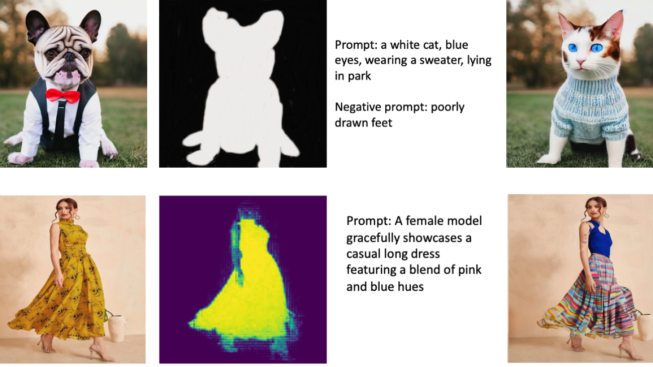
The following images are examples of inpainting. The original images are on the left, the mask image is in the center, and the inpainted image generated by the model is on the right. For the first example, the model was provided with the original image, a mask image, and the textual prompt “a white cat, blue eyes, wearing a sweater, lying in park,” as well as the negative prompt “poorly drawn feet.” For the second example, the textual prompt was “A female model gracefully showcases a casual long dress featuring a blend of pink and blue hues,”

Running large models like Stable Diffusion requires custom inference scripts. You have to run end-to-end tests to make sure that the script, the model, and the desired instance work together efficiently. JumpStart simplifies this process by providing ready-to-use scripts that have been robustly tested. You can access these scripts with one click through the Studio UI or with very few lines of code through the JumpStart APIs.
The following sections guide you through deploying the model and running inference using either the Studio UI or the JumpStart APIs.
Note that by using this model, you agree to the CreativeML Open RAIL++-M License.
Access JumpStart through the Studio UI
In this section, we illustrate the deployment of JumpStart models using the Studio UI. The accompanying video demonstrates locating the pre-trained Stable Diffusion inpainting model on JumpStart and deploying it. The model page offers essential details about the model and its usage. To perform inference, we employ the ml.p3.2xlarge instance type, which delivers the required GPU acceleration for low-latency inference at an affordable price. After the SageMaker hosting instance is configured, choose Deploy. The endpoint will be operational and prepared to handle inference requests within approximately 10 minutes.
JumpStart provides a sample notebook that can help accelerate the time it takes to run inference on the newly created endpoint. To access the notebook in Studio, choose Open Notebook in the Use Endpoint from Studio section of the model endpoint page.
Use JumpStart programmatically with the SageMaker SDK
Utilizing the JumpStart UI enables you to deploy a pre-trained model interactively with only a few clicks. Alternatively, you can employ JumpStart models programmatically by using APIs integrated within the SageMaker Python SDK.
In this section, we choose an appropriate pre-trained model in JumpStart, deploy this model to a SageMaker endpoint, and perform inference on the deployed endpoint, all using the SageMaker Python SDK. The following examples contain code snippets. To access the complete code with all the steps included in this demonstration, refer to the Introduction to JumpStart Image editing – Stable Diffusion Inpainting example notebook.
Deploy the pre-trained model
SageMaker utilizes Docker containers for various build and runtime tasks. JumpStart utilizes the SageMaker Deep Learning Containers (DLCs) that are framework-specific. We first fetch any additional packages, as well as scripts to handle training and inference for the selected task. Then the pre-trained model artifacts are separately fetched with model_uris, which provides flexibility to the platform. This allows multiple pre-trained models to be used with a single inference script. The following code illustrates this process:
Next, we provide those resources to a SageMaker model instance and deploy an endpoint:
After the model is deployed, we can obtain real-time predictions from it!
Input
The input is the base image, a mask image, and the prompt describing the subject, object, or environment to be substituted in the masked-out portion. Creating the perfect mask image for in-painting effects involves several best practices. Start with a specific prompt, and don’t hesitate to experiment with various Stable Diffusion settings to achieve desired outcomes. Utilize a mask image that closely resembles the image you aim to inpaint. This approach aids the inpainting algorithm in completing the missing sections of the image, resulting in a more natural appearance. High-quality images generally yield better results, so make sure your base and mask images are of good quality and resemble each other. Additionally, opt for a large and smooth mask image to preserve detail and minimize artifacts.
The endpoint accepts the base image and mask as raw RGB values or a base64 encoded image. The inference handler decodes the image based on content_type:
- For
content_type = “application/json”, the input payload must be a JSON dictionary with the raw RGB values, textual prompt, and other optional parameters - For
content_type = “application/json;jpeg”, the input payload must be a JSON dictionary with the base64 encoded image, a textual prompt, and other optional parameters
Output
The endpoint can generate two types of output: a Base64-encoded RGB image or a JSON dictionary of the generated images. You can specify which output format you want by setting the accept header to "application/json" or "application/json;jpeg" for a JPEG image or base64, respectively.
- For
accept = “application/json”, the endpoint returns the a JSON dictionary with RGB values for the image - For
accept = “application/json;jpeg”, the endpoint returns a JSON dictionary with the JPEG image as bytes encoded with base64.b64 encoding
Note that sending or receiving the payload with the raw RGB values may hit default limits for the input payload and the response size. Therefore, we recommend using the base64 encoded image by setting content_type = “application/json;jpeg” and accept = “application/json;jpeg”.
The following code is an example inference request:
Supported parameters
Stable Diffusion inpainting models support many parameters for image generation:
- image – The original image.
- mask – An image where the blacked-out portion remains unchanged during image generation and the white portion is replaced.
- prompt – A prompt to guide the image generation. It can be a string or a list of strings.
- num_inference_steps (optional) – The number of denoising steps during image generation. More steps lead to higher quality image. If specified, it must be a positive integer. Note that more inference steps will lead to a longer response time.
- guidance_scale (optional) – A higher guidance scale results in an image more closely related to the prompt, at the expense of image quality. If specified, it must be a float.
guidance_scale<=1is ignored. - negative_prompt (optional) – This guides the image generation against this prompt. If specified, it must be a string or a list of strings and used with
guidance_scale. Ifguidance_scaleis disabled, this is also disabled. Moreover, if the prompt is a list of strings, then thenegative_promptmust also be a list of strings. - seed (optional) – This fixes the randomized state for reproducibility. If specified, it must be an integer. Whenever you use the same prompt with the same seed, the resulting image will always be the same.
- batch_size (optional) – The number of images to generate in a single forward pass. If using a smaller instance or generating many images, reduce
batch_sizeto be a small number (1–2). The number of images = number of prompts*num_images_per_prompt.
Limitations and biases
Even though Stable Diffusion has impressive performance in inpainting, it suffers from several limitations and biases. These include but are not limited to:
- The model may not generate accurate faces or limbs because the training data doesn’t include sufficient images with these features.
- The model was trained on the LAION-5B dataset, which has adult content and may not be fit for product use without further considerations.
- The model may not work well with non-English languages because the model was trained on English language text.
- The model can’t generate good text within images.
- Stable Diffusion inpainting typically works best with images of lower resolutions, such as 256×256 or 512×512 pixels. When working with high-resolution images (768×768 or higher), the method might struggle to maintain the desired level of quality and detail.
- Although the use of a seed can help control reproducibility, Stable Diffusion inpainting may still produce varied results with slight alterations to the input or parameters. This might make it challenging to fine-tune the output for specific requirements.
- The method might struggle with generating intricate textures and patterns, especially when they span large areas within the image or are essential for maintaining the overall coherence and quality of the inpainted region.
For more information on limitations and bias, refer to the Stable Diffusion Inpainting model card.
Inpainting solution with mask generated via a prompt
CLIPSeq is an advanced deep learning technique that utilizes the power of pre-trained CLIP (Contrastive Language-Image Pretraining) models to generate masks from input images. This approach provides an efficient way to create masks for tasks such as image segmentation, inpainting, and manipulation. CLIPSeq uses CLIP to generate a text description of the input image. The text description is then used to generate a mask that identifies the pixels in the image that are relevant to the text description. The mask can then be used to isolate the relevant parts of the image for further processing.
CLIPSeq has several advantages over other methods for generating masks from input images. First, it’s a more efficient method, because it doesn’t require the image to be processed by a separate image segmentation algorithm. Second, it’s more accurate, because it can generate masks that are more closely aligned with the text description of the image. Third, it’s more versatile, because you can use it to generate masks from a wide variety of images.
However, CLIPSeq also has some disadvantages. First, the technique may have limitations in terms of subject matter, because it relies on pre-trained CLIP models that may not encompass specific domains or areas of expertise. Second, it can be a sensitive method, because it’s susceptible to errors in the text description of the image.
For more information, refer to Virtual fashion styling with generative AI using Amazon SageMaker.
Clean up
After you’re done running the notebook, make sure to delete all resources created in the process to ensure that the billing is stopped. The code to clean up the endpoint is available in the associated notebook.
Conclusion
In this post, we showed how to deploy a pre-trained Stable Diffusion inpainting model using JumpStart. We showed code snippets in this post—the full code with all of the steps in this demo is available in the Introduction to JumpStart – Enhance image quality guided by prompt example notebook. Try out the solution on your own and send us your comments.
To learn more about the model and how it works, see the following resources:
- High-Resolution Image Synthesis with Latent Diffusion Models
- Stable Diffusion Launch Announcement
- Stable Diffusion 2.0 Release
- Stable Diffusion Inpainting model card
To learn more about JumpStart, check out the following posts:
- Generate images from text with the stable diffusion model on Amazon SageMaker JumpStart
- Upscale images with Stable Diffusion in Amazon SageMaker JumpStart
- AlexaTM 20B is now available in Amazon SageMaker JumpStart
- Run text generation with Bloom and GPT models on Amazon SageMaker JumpStart
- Run image segmentation with Amazon SageMaker JumpStart
- Run text classification with Amazon SageMaker JumpStart using TensorFlow Hub and Hugging Face models
- Amazon SageMaker JumpStart models and algorithms now available via API
- Incremental training with Amazon SageMaker JumpStart
- Transfer learning for TensorFlow object detection models in Amazon SageMaker
- Transfer learning for TensorFlow text classification models in Amazon SageMaker
- Transfer learning for TensorFlow image classification models in Amazon SageMaker
About the Authors
 Dr. Vivek Madan is an Applied Scientist with the Amazon SageMaker JumpStart team. He got his PhD from University of Illinois at Urbana-Champaign and was a Post Doctoral Researcher at Georgia Tech. He is an active researcher in machine learning and algorithm design and has published papers in EMNLP, ICLR, COLT, FOCS, and SODA conferences.
 Alfred Shen is a Senior AI/ML Specialist at AWS. He has been working in Silicon Valley, holding technical and managerial positions in diverse sectors including healthcare, finance, and high-tech. He is a dedicated applied AI/ML researcher, concentrating on CV, NLP, and multimodality. His work has been showcased in publications such as EMNLP, ICLR, and Public Health.
Deploy large language models on AWS Inferentia2 using large model inference containers
You don’t have to be an expert in machine learning (ML) to appreciate the value of large language models (LLMs). Better search results, image recognition for the visually impaired, creating novel designs from text, and intelligent chatbots are just some examples of how these models are facilitating various applications and tasks.
ML practitioners keep improving the accuracy and capabilities of these models. As a result, these models grow in size and generalize better, such as in the evolution of transformer models. We explained in a previous post how you can use Amazon SageMaker deep learning containers (DLCs) to deploy these kinds of large models using a GPU-based instance.
In this post, we take the same approach but host the model on AWS Inferentia2. We use the AWS Neuron software development kit (SDK) to access the Inferentia device and benefit from its high performance. We then use a large model inference container powered by Deep Java Library (DJLServing) as our model serving solution. We demonstrate how these three layers work together by deploying an OPT-13B model on an Amazon Elastic Compute Cloud (Amazon EC2) inf2.48xlarge instance.
The three pillars
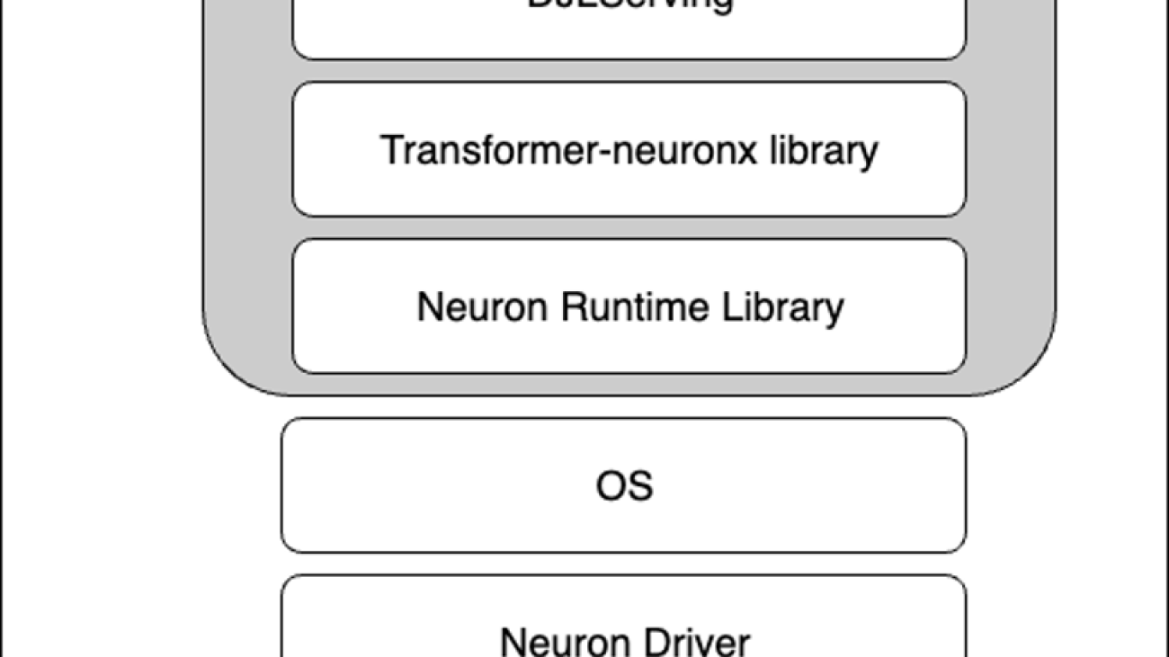
The following image represents the layers of hardware and software working to help you unlock the best price and performance of your large language models. AWS Neuron and tranformer-neuronx are the SDKs used to run deep learning workloads on AWS Inferentia. Lastly, DJLServing is the serving solution that is integrated in the container.

Hardware: Inferentia
AWS Inferentia, specifically designed for inference by AWS, is a high-performance and low-cost ML inference accelerator. In this post, we use AWS Inferentia2 (available via Inf2 instances), the second generation purpose-built ML inference accelerator.
Each EC2 Inf2 instance is powered by up to 12 Inferentia2 devices, and allows you to choose between four instance sizes.
Amazon EC2 Inf2 supports NeuronLink v2, a low-latency and high-bandwidth chip-to-chip interconnect, which enables high performance collective communication operations such as AllReduce and AllGather. This efficiently shards models across AWS Inferentia2 devices (such as via Tensor Parallelism), and therefore optimizes latency and throughput. This is particularly useful for large language models. For benchmark performance figures, refer to AWS Neuron Performance.

At the heart of the Amazon EC2 Inf2 instance are AWS Inferentia2 devices, each containing two NeuronCores-v2. Each NeuronCore-v2 is an independent, heterogenous compute-unit, with four main engines: Tensor, Vector, Scalar, and GPSIMD engines. It includes an on-chip software-managed SRAM memory for maximizing data locality. The following diagram shows the internal workings of the AWS Inferentia2 device architecture.

Neuron and transformers-neuronx
Above the hardware layer are the software layers used to interact with AWS Inferentia. AWS Neuron is the SDK used to run deep learning workloads on AWS Inferentia and AWS Trainium based instances. It enables end-to-end ML development lifecycle to build new models, train and optimize these models, and deploy them for production. AWS Neuron includes a deep learning compiler, runtime, and tools that are natively integrated with popular frameworks like TensorFlow and PyTorch.
transformers-neuronx is an open-source library built by the AWS Neuron team that helps run transformer decoder inference workflows using the AWS Neuron SDK. Currently, it has examples for the GPT2, GPT-J, and OPT model types, and different model sizes that have their forward functions re-implemented in a compiled language for extensive code analysis and optimizations. Customers can implement other model architecture based on the same library. AWS Neuron-optimized transformer decoder classes have been re-implemented in XLA HLO (High Level Operations) using a syntax called PyHLO. The library also implements tensor parallelism to shard the model weights across multiple NeuronCores.
Tensor parallelism is needed because the models are so large, they don’t fit into a single accelerator HBM memory. The support for tensor parallelism by the AWS Neuron runtime in transformers-neuronx makes heavy use of collective operations such as AllReduce. The following are some principles for setting the tensor parallelism degree (number of NeuronCores participating in sharded matrix multiply operations) for AWS Neuron-optimized transformer decoder models:
- The number of attention heads needs to be divisible by the tensor parallelism degree
- The total data size of model weights and key-value caches needs to be smaller than 16 GB times the tensor parallelism degree
- Currently, the Neuron runtime supports tensor parallelism degrees 1, 2, 8, and 32 on Trn1 and supports tensor parallelism degrees 1, 2, 4, 8, and 24 on Inf2
DJLServing
DJLServing is a high-performance model server that added support for AWS Inferentia2 in March 2023. The AWS Model Server team offers a container image that can help LLM/AIGC use cases. DJL is also part of Rubikon support for Neuron that includes the integration between DJLServing and transformers-neuronx. The DJLServing model server and transformers-neuronx library are the core components of the container built to serve the LLMs supported through the transformers library. This container and the subsequent DLCs will be able to load the models on the AWS Inferentia chips on an Amazon EC2 Inf2 host along with the installed AWSInferentia drivers and toolkit. In this post, we explain two ways of running the container.
The first way is to run the container without writing any additional code. You can use the default handler for a seamless user experience and pass in one of the supported model names and any load time configurable parameters. This will compile and serve an LLM on an Inf2 instance. The following code shows an example:
engine=Python
option.entryPoint=djl_python.transformers_neuronx
option.task=text-generation
option.model_id=facebook/opt-1.3b
option.tensor_parallel_degree=2
Alternatively, you can write your own model.py file, but that requires implementing the model loading and inference methods to serve as a bridge between the DJLServing APIs and, in this case, the transformers-neuronx APIs. You can also provide configurable parameters in a serving.properties file to be picked up during model loading. For the full list of configurable parameters, refer to All DJL configuration options.
The following code is a sample model.py file. The serving.properties file is similar to the one shown earlier.
def load_model(properties):
     """
    Load a model based from the framework provided APIs
    :param: properties configurable properties for model loading
            specified in serving.properties
    :return: model and other artifacts required for inference
    """
    batch_size = int(properties.get("batch_size", 2))
    tp_degree = int(properties.get("tensor_parallel_degree", 2))
    amp = properties.get("dtype", "f16")

    model_id = "facebook/opt-13b"
    model = OPTForCausalLM.from_pretrained(model_id, low_cpu_mem_usage=True)
    ...

    tokenizer = AutoTokenizer.from_pretrained(model_id)
    model = OPTForSampling.from_pretrained(load_path,
                                           batch_size=batch_size,
                                           amp=amp,
                                           tp_degree=tp_degree)
    model.to_neuron()
    return model, tokenizer, batch_size
Let’s see what this all looks like on an Inf2 instance.
Launch the Inferentia hardware
We first need to launch an inf.42xlarge instance to host our OPT-13b model. We use the Deep Learning AMI Neuron PyTorch 1.13.0 (Ubuntu 20.04) 20230226 Amazon Machine Image (AMI) because it already includes the Docker image and necessary drivers for the AWS Neuron runtime.

We increase the storage of the instance to 512 GB to accommodate for large language models.

Install necessary dependencies and create the model
We set up a Jupyter notebook server with our AMI to make it easier to view and manage our directories and files. When we’re in the desired directory, we set subdirectories for logs and models and create a serving.properties file.

We can use the standalone model provided by the DJL Serving container. This means we don’t have to define a model, but we do need to provide a serving.properties file. See the following code:
option.model_id=facebook/opt-1.3b
option.batch_size=2
option.tensor_parallel_degree=2
option.n_positions=256
option.dtype=fp16
option.model_loading_timeout=600
engine=Python
option.entryPoint=djl_python.transformers-neuronx
#option.s3url=s3://djl-llm/opt-1.3b/

#can also specify which device to load on.
#engine=Python ---because the handles are implement in python.
This instructs the DJL model server to use the OPT-13B model. We set the batch size to 2 and dtype=f16 for the model to fit on the neuron device. DJL serving supports dynamic batching and by setting a similar tensor_parallel_degree value, we can increase throughput of inference requests because we distribute inference across multiple NeuronCores. We also set n_positions=256 because this informs the maximum length we expect the model to have.
Our instance has 12 AWS Neuron devices, or 24 NeuronCores, while our OPT-13B model requires 40 attention heads. For example, setting tensor_parallel_degree=8 means every 8 NeuronCores will host one model instance. If you divide the required attention heads (40) by the number of NeuronCores (8), then you get 5 attention heads allocated to each NeuronCore, or 10 on each AWS Neuron device.
You can use the following sample model.py file, which defines the model and creates the handler function. You can edit it to meet your needs, but be sure it can be supported on transformers-neuronx.
cat serving.propertiesoption.tensor_parallel_degree=2
option.batch_size=2
option.dtype=f16
engine=Pythoncat model.pyimport torch
import tempfile
import os
from transformers.models.opt import OPTForCausalLM
from transformers import AutoTokenizer
from transformers_neuronx import dtypes
from transformers_neuronx.module import save_pretrained_split
from transformers_neuronx.opt.model import OPTForSampling
from djl_python import Input, Output
model = None
def load_model(properties):
batch_size = int(properties.get("batch_size", 2))
tp_degree = int(properties.get("tensor_parallel_degree", 2))
amp = properties.get("dtype", "f16")
model_id = "facebook/opt-13b"
load_path = os.path.join(tempfile.gettempdir(), model_id)
model = OPTForCausalLM.from_pretrained(model_id,
low_cpu_mem_usage=True)
dtype = dtypes.to_torch_dtype(amp)
for block in model.model.decoder.layers:
block.self_attn.to(dtype)
block.fc1.to(dtype)
block.fc2.to(dtype)
model.lm_head.to(dtype)
save_pretrained_split(model, load_path)
tokenizer = AutoTokenizer.from_pretrained(model_id)
model = OPTForSampling.from_pretrained(load_path,
batch_size=batch_size,
amp=amp,
tp_degree=tp_degree)
model.to_neuron()
return model, tokenizer, batch_size
def infer(seq_length, prompt):
with torch.inference_mode():
input_ids = torch.as_tensor([tokenizer.encode(text) for text in prompt])
generated_sequence = model.sample(input_ids,
sequence_length=seq_length)
outputs = [tokenizer.decode(gen_seq) for gen_seq in generated_sequence]
return outputs
def handle(inputs: Input):
global model, tokenizer, batch_size
if not model:
model, tokenizer, batch_size = load_model(inputs.get_properties())
if inputs.is_empty():
# Model server makes an empty call to warmup the model on startup
return None
data = inputs.get_as_json()
seq_length = data["seq_length"]
prompt = data["text"]
outputs = infer(seq_length, prompt)
result = {"outputs": outputs}
return Output().add_as_json(result)
mkdir -p models/opt13b logs
mv serving.properties model.py models/opt13b
Run the serving container
The last steps before inference are to pull the Docker image for the DJL serving container and run it on our instance:
docker pull deepjavalibrary/djl-serving:0.21.0-pytorch-inf2After you pull the container image, run the following command to deploy your model. Make sure you’re in the right directory that contains the logs and models subdirectory because the command will map these to the container’s /opt/directories.
docker run -it --rm --network=host
           -v `pwd`/models:/opt/ml/model
           -v `pwd`/logs:/opt/djl/logs
           -u djl --device /dev/neuron0  --device /dev/neuron10  --device /dev/neuron2  --device /dev/neuron4  --device /dev/neuron6  --device /dev/neuron8 --device /dev/neuron1  --device /dev/neuron11
           -e MODEL_LOADING_TIMEOUT=7200
           -e PREDICT_TIMEOUT=360
           deepjavalibrary/djl-serving:0.21.0-pytorch-inf2 serve
Run inference
Now that we’ve deployed the model, let’s test it out with a simple CURL command to pass some JSON data to our endpoint. Because we set a batch size of 2, we pass along the corresponding number of inputs:
curl -X POST "http://127.0.0.1:8080/predictions/opt13b"
     -H 'Content-Type: application/json'
     -d '{"seq_length":2048,
          "text":[
                    "Hello, I am a language model,",
                    "Welcome to Amazon Elastic Compute Cloud,"
                  ]
          }'
The preceding command generates a response in the command line. The model is quite chatty but its response validates our model. We were able to run inference on our LLM thanks to Inferentia!
Clean up
Don’t forget to delete your EC2 instance once you are done to save cost.
Conclusion
In this post, we deployed an Amazon EC2 Inf2 instance to host an LLM and ran inference using a large model inference container. You learned how AWS Inferentia and the AWS Neuron SDK interact to allow you to easily deploy LLMs for inference at an optimal price-to-performance ratio. Stay tuned for updates on more capabilities and new innovations with Inferentia. For more examples about Neuron, see aws-neuron-samples.
About the Authors
 Qingwei Li is a Machine Learning Specialist at Amazon Web Services. He received his Ph.D. in Operations Research after he broke his advisor’s research grant account and failed to deliver the Nobel Prize he promised. Currently he helps customers in the financial service and insurance industry build machine learning solutions on AWS. In his spare time, he likes reading and teaching.
 Peter Chung is a Solutions Architect for AWS, and is passionate about helping customers uncover insights from their data. He has been building solutions to help organizations make data-driven decisions in both the public and private sectors. He holds all AWS certifications as well as two GCP certifications. He enjoys coffee, cooking, staying active, and spending time with his family.
 Aaqib Ansari is a Software Development Engineer with the Amazon SageMaker Inference team. He focuses on helping SageMaker customers accelerate model inference and deployment. In his spare time, he enjoys hiking, running, photography and sketching.
 Qing Lan is a Software Development Engineer in AWS. He has been working on several challenging products in Amazon, including high performance ML inference solutions and high performance logging system. Qing’s team successfully launched the first Billion-parameter model in Amazon Advertising with very low latency required. Qing has in-depth knowledge on the infrastructure optimization and Deep Learning acceleration.
 Frank Liu is a Software Engineer for AWS Deep Learning. He focuses on building innovative deep learning tools for software engineers and scientists. In his spare time, he enjoys hiking with friends and family.
Building toward more autonomous and proactive cloud technologies with AI

Cloud Intelligence/AIOps blog series
In the first blog post in this series, Cloud Intelligence/AIOps – Infusing AI into Cloud Computing Systems, we presented a brief overview of Microsoft’s research on Cloud Intelligence/AIOps (AIOps), which innovates AI and machine learning (ML) technologies to help design, build, and operate complex cloud platforms and services effectively and efficiently at scale. As cloud computing platforms have continued to emerge as one of the most fundamental infrastructures of our world, both their scale and complexity have grown considerably. In our previous blog post, we discussed the three major pillars of AIOps research: AI for Systems, AI for Customers, and AI for DevOps, as well as the four major research areas that constitute the AIOps problem space: detection, diagnosis, prediction, and optimization. We also envisioned the AIOps research roadmap as building toward creating more autonomous, proactive, manageable, and comprehensive cloud platforms.
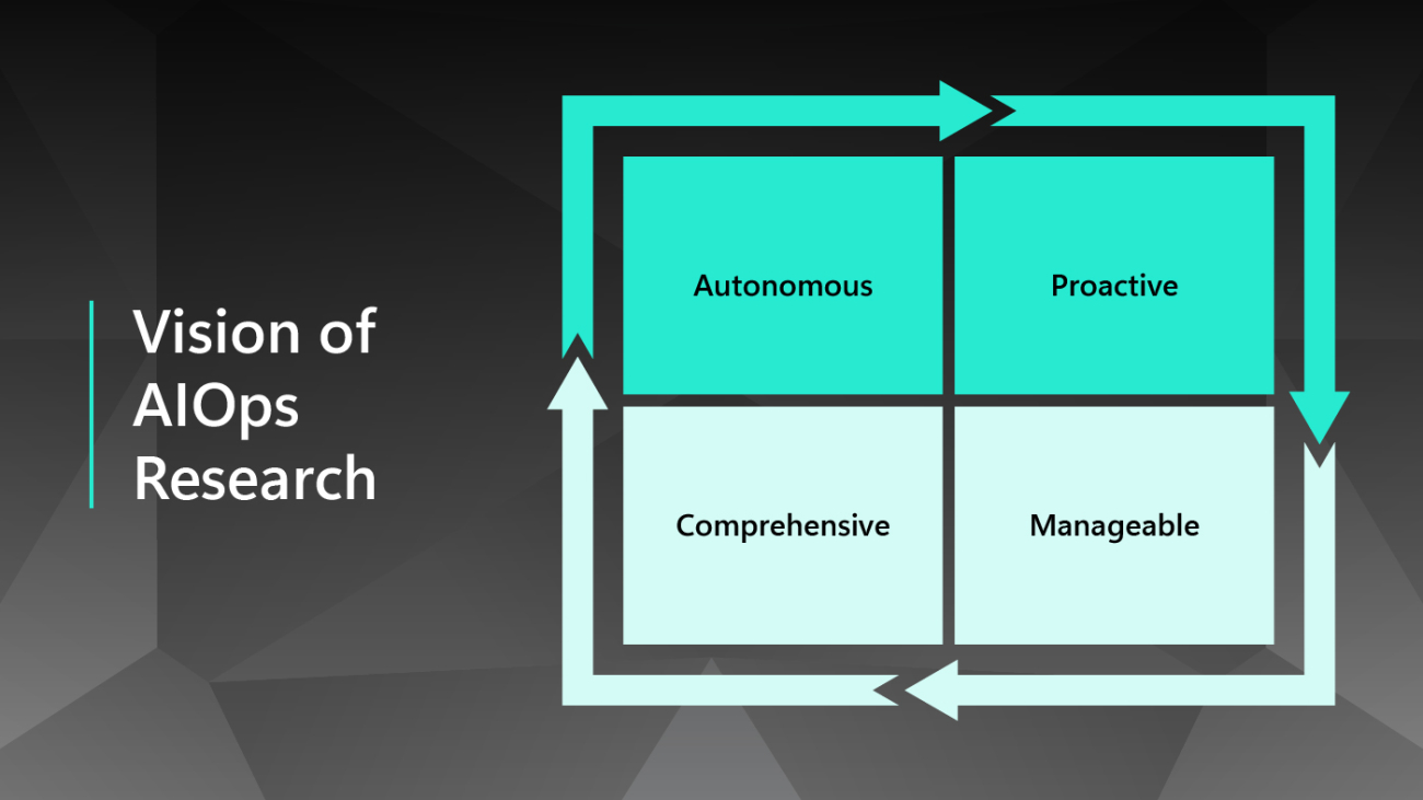
Vision of AIOps Research
| Autonomous | Proactive | Manageable | Comprehensive |
| Fully automate the operation of cloud systems to minimize system downtime and reduce manual efforts. | Predict future cloud status, support proactive decision-making, and prevent bad things from happening. | Introduce the notion of tiered autonomy for infusing autonomous routine operations and deep human expertise. | Span AIOps to the full cloud stack for global optimization/management and extend to multi-cloud environments. |
Starting with this blog post, we will take a deeper dive into Microsoft’s vision for AIOps research and the ongoing efforts to realize that vision. This blog post will focus on how our researchers leveraged state-of-the-art AIOps research to help make cloud technologies more autonomous and proactive. We will discuss our work to make the cloud more manageable and comprehensive in future blog posts.
Autonomous cloud
Motivation
Cloud platforms require numerous actions and decisions every second to ensure that computing resources are properly managed and failures are promptly addressed. In practice, those actions and decisions are either generated by rule-based systems constructed upon expert knowledge or made manually by experienced engineers. Still, as cloud platforms continue to grow in both scale and complexity, it is apparent that such solutions will be insufficient for the future cloud system. On one hand, rigid rule-based systems, while being knowledge empowered, often involve huge numbers of rules and require frequent maintenance for better coverage and adaptability. Still, in practice, it is often unrealistic to keep such systems up to date as cloud systems expand in both size and complexity, and even more difficult to guarantee consistency and avoid conflicts between all the rules. On the other hand, engineering efforts are very time-consuming, prone to errors, and difficult to scale.
Spotlight: Microsoft Research Podcast
AI Frontiers: The Physics of AI with Sébastien Bubeck
What is intelligence? How does it emerge and how do we measure it? Ashley Llorens and machine learning theorist Sébastian Bubeck discuss accelerating progress in large-scale AI and early experiments with GPT-4.
To break the constraints on the coverage and scalability of the existing solutions and improve the adaptability and manageability of the decision-making systems, cloud platforms must shift toward a more autonomous management paradigm. Instead of relying solely on expert knowledge, we need suitable AI/ML models to fuse operational data and expert knowledge together to enable efficient, reliable, and autonomous management decisions. Still, it will take many research and engineering efforts to overcome various barriers for developing and deploying autonomous solutions to cloud platforms.
Toward an autonomous cloud
In the journey towards an autonomous cloud, there are two major challenges. The first challenge lies in the heterogeneity of cloud data. In practice, cloud platforms deploy a huge number of monitors to collect data in various formats, including telemetry signals, machine-generated log files, and human input from engineers and users. And the patterns and distributions of those data generally exhibit a high degree of diversity and are subjected to changes over time. To ensure that the adopted AIOps solutions can function autonomously in such an environment, it is essential to empower the management system with robust and extendable AI/ML models capable of learning useful information from heterogeneous data sources and drawing right conclusions in various scenarios.
The complex interaction between different components and services presents another major challenge in deploying autonomous solutions. While it can be easy to implement autonomous features for one or a few components/services, how to construct end-to-end systems capable of automatically navigating the complex dependencies in cloud systems presents the true challenge for both researchers and engineers. To address this challenge, it is important to leverage both domain knowledge and data to optimize the automation paths in application scenarios. Researchers and engineers should also implement reliable decision-making algorithms in every decision stage to improve the efficiency and stability of the whole end-to-end decision-making process.
Over the past few years, Microsoft research groups have developed many new models and methods for overcoming those challenges and improving the level of automation in various cloud application scenarios across the AIOps problem spaces. Notable examples include:
- Detection: Gandalf and ATAD for the early detection of problematic deployments; HALO for hierarchical faulty localization; and Onion for detecting incident-indicating logs.
- Diagnosis: SPINE and UniParser for log parsing; Logic and Warden for regression and incident diagnosis; and CONAN for batch failure diagnosis.
- Prediction: TTMPred for predicting time to mitigate incidents; LCS for predicting the low-capacity status in cloud servers; and Eviction Prediction for predicting the eviction of spot virtual machines.
- Optimization: MLPS for optimizing the reallocation of containers; and RESIN for the management of memory leak in cloud infrastructure.
These solutions not only improve service efficiency and reduce management time with more automatous design, but also result in higher performance and reliability with fewer human errors. As an illustration of our work toward a more autonomous cloud, we will discuss our exploration for supporting automatic safe deployment services below.
Exemplary scenario: Automatic safe deployment
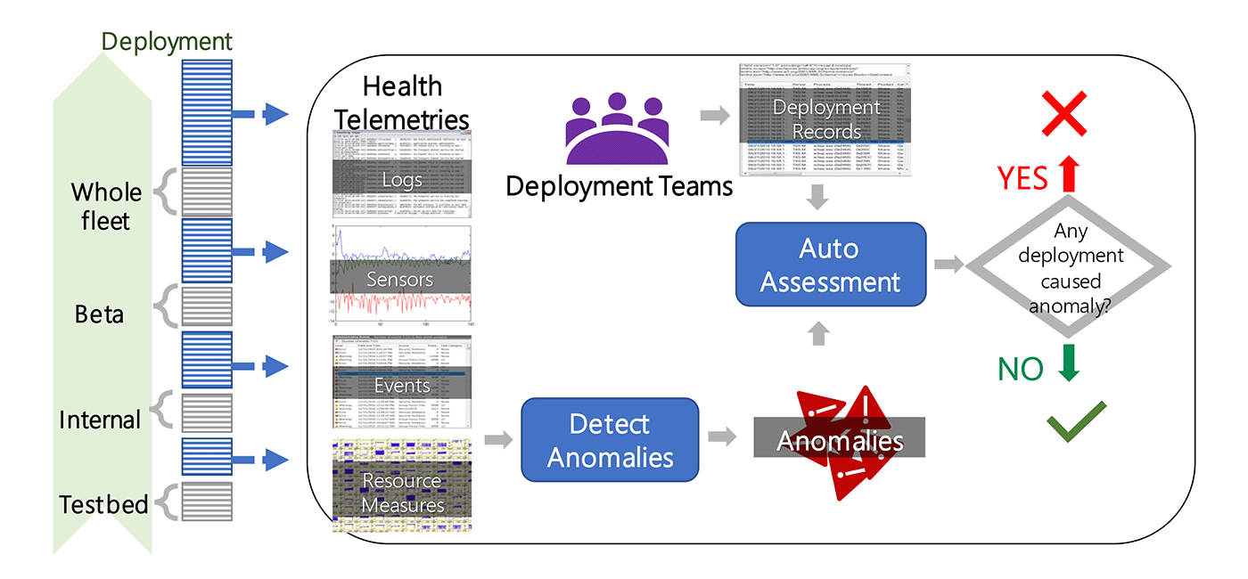
In online services, the continuous integration and continuous deployment (CI/CD) of new patches and builds are critical for the timely delivery of bug fixes and feature updates. Because new deployments with undetected bugs or incompatible issues can cause severe service outages and create significant customer impact, cloud platforms enforce strict safe-deployment procedures before releasing each new deployment to the production environments. Such procedures typically involve multi-stage testing and verification in a sequence of canary environments with increasing scopes. When a deployment-related anomaly is identified in one of these stages, the responsible deployment is rolled back for further diagnosis and fixing. Owing to the challenges of identifying deployment-related anomalies with heterogeneous patterns and managing a huge number of deployments, safe-deployment systems administrated manually can be extremely costly and error prone.
To support automatic and reliable anomaly detection in safe deployment, we proposed a general methodology named ATAD for the effective detection of deployment-related anomalies in time-series signals. This method addresses the challenges of capturing changes with various patterns in time-series signals and the lack of labeled anomaly samples due to the heavy cost of labeling. Specifically, this method combines ideas from both transfer learning and active learning to make good use of the temporal information in the input signal and reduce the number of labeled samples required for model training. Our experiments have shown that ATAD can outperform other state-of-the-art anomaly detection approaches, even with only 1%-5% of labeled data.
At the same time, we collaborated with product teams in Azure to develop and deploy Gandalf, an end-to-end automatic safe deployment system that reduces deployment time and increases the accuracy of detecting bad deployment in Azure. As a data-driven system, Gandalf monitors a large array of information, including performance metrics, failure signals and deployment records. It also detects anomalies in various patterns throughout the entire safe-deployment process. After detecting anomalies, Gandalf applies a vote-veto mechanism to reliably determine whether each detected anomaly is caused by a specific new deployment. Gandalf then automatically decides whether the relevant new deployment should be stopped for a fix or if it’s safe enough to proceed to the next stage. After rolling out in Azure, Gandalf has been effective at helping to capture bad deployments, achieving more than 90% precision and near 100% recall in production over a period of 18 months.
Proactive cloud
Motivation
Traditional decision-making in the cloud focuses on optimizing immediate resource usage and addressing emerging issues. While this reactive design is not unreasonable in a relatively static system, it can lead to short-sighted decisions in a dynamic environment. In cloud platforms, both the demand and utilization of computing resources are undergoing constant changes, including regular periodical patterns, unexpected spikes, and gradual shifts in both temporal and spatial dimensions. To improve the long-term efficiency and reliability of cloud platforms, it is critical to adopt a proactive design that takes the future status of the system into account in the decision-making process.
A proactive design leverages data-driven models to predict the future status of cloud platforms and enable downstream proactive decision-making. Conceptually, a typical proactive decision-making system consists of two modules: a prediction module and a decision-making module, as displayed in the following diagram.
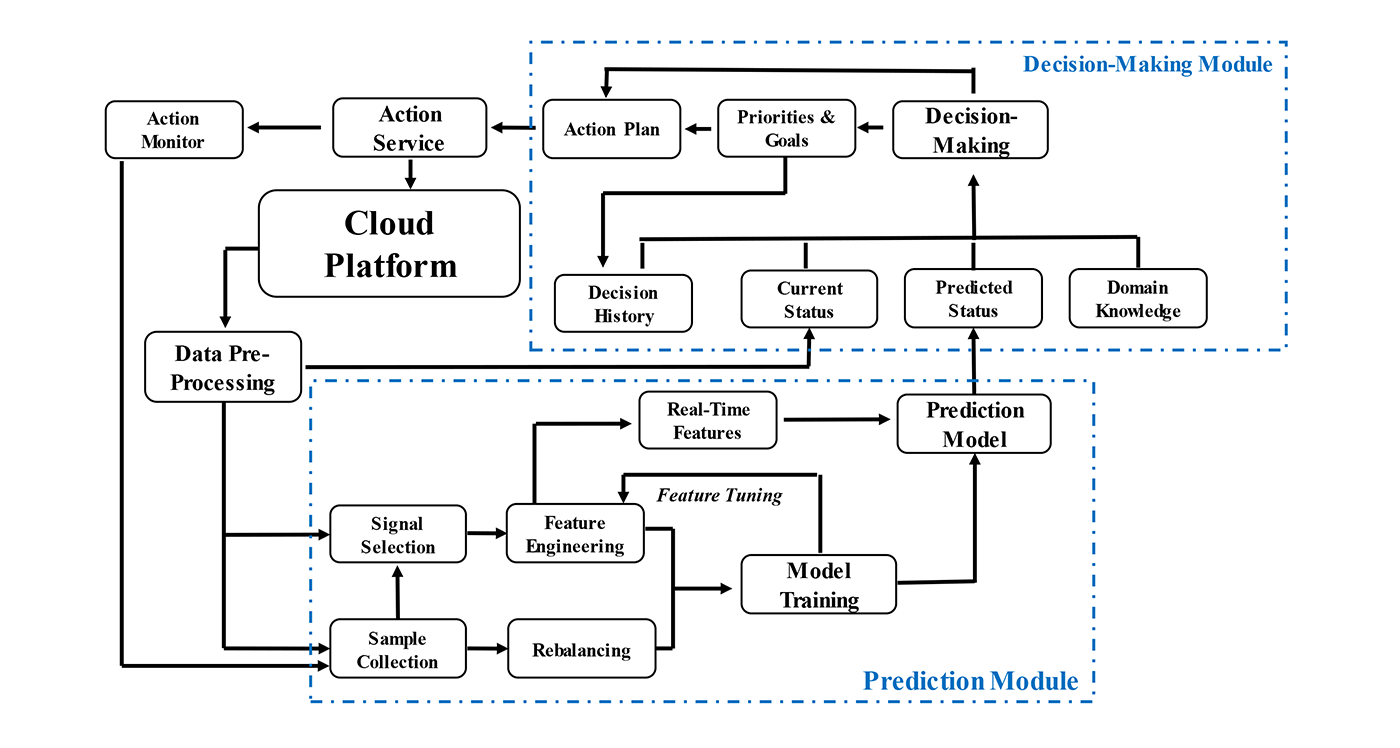
In the prediction module, historical data are collected and processed for training and fine-tuning the prediction model for deployment. The deployed prediction model takes in the online data stream and generates prediction results in real time. In the decision-making module, both the current system status and the predicted system status, along with other information such as domain knowledge and past decision history, is considered for making decisions that balance both present and future benefits.
Toward proactive design
Proactive design, while creating new opportunities for improving the long-term efficiency and reliability of cloud systems, does expose the decision-making process to additional risks. On one hand, thanks to the inherent randomness in the daily operation of cloud platforms, proactive decisions are always subjected to the uncertainty risk from the stochastic elements in both running systems and the environments. On the other hand, the reliability of prediction models adds another layer of risks in making proactive decisions. Therefore, to guarantee the performance of proactive design, engineers must put mechanisms in place to address those risks.
To manage uncertainty risk, engineers need to reformulate the decision-making in proactive design to account for the uncertainty elements. They can often use methodological frameworks, such as prediction+optimization and optimization under chance-constraints, to incorporate uncertainties into the target functions of optimization problems. Well-designed ML/AL models can also learn uncertainty from data for improving proactive decisions against uncertainty elements. As for risks associated with the prediction model, modules for improving data quality, including quality-aware feature engineering, robust data imputation, and data rebalancing, should be applied to reduce prediction errors. Engineers should also make continuous efforts to improve and update the robustness of prediction models. Moreover, safeguarding mechanisms are essential to prevent decisions that may cause harm to the cloud system.
Microsoft’s AIOps research has pioneered the transition from reactive decision-making to proactive decision-making, especially in problem spaces of prediction and optimization. Our efforts not only lead to significant improvement in many application scenarios traditionally supported by reactive decision-making, but also create many new opportunities. Notable proactive design solutions include Narya and Nenya for hardware failure mitigation, UAHS and CAHS for the intelligent virtual machine provisioning, CUC for the predictive scheduling of workloads, and UCaC for bin packing optimization under chance constraints. In the discussion below, we will use hardware failure mitigation as an example to illustrate how proactive design can be applied in cloud scenarios.
Exemplary scenario: Proactive hardware failure mitigation
A key threat to cloud platforms is hardware failure, which can cause interruptions to the hosted services and significantly impact the customer experience. Traditionally, hardware failures are only resolved reactively after the failure occurs, which typically involves temporal interruptions of hosted virtual machines and the repair or replacement of impacted hardware. Such a solution provides limited help in reducing negative customer experiences.
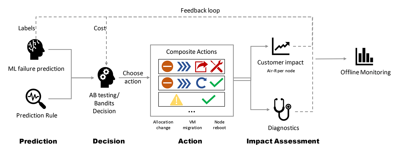
Narya is a proactive disk-failure mitigation service capable of taking mitigation actions before failures occur. Specifically, Narya leverages ML models to predict potential disk failures, and then make decisions accordingly. To control risks associated with uncertainty, Narya evaluates candidate mitigation actions based on the estimated impacts to customers and chooses actions with minimum impact. A feedback loop also exists for collecting follow-up assessments to improve prediction and decision modules.
Hardware failures in cloud systems are often highly interdependent. Therefore, to reduce the impact of predictions errors, Narya introduces a novel dependency-aware model to encode the dependency relationship between nodes to improve the failure prediction model. Narya also implements an adaptive approach that uses A/B testing and bandit modeling to improve the ability to estimate the impacts of actions. Several safeguarding mechanisms in different stages of Narya are also in place to eliminate the chance of making unsafe mitigation actions. Implementation of Narya in Azure’s production environment has reduced the node hardware interruption rate for virtual machines by more than 26%.
Our recent work, Nenya, is another example for proactive failure mitigation. Under a reinforcement learning framework, Nenya fuses prediction and decision-making modules into an end-to-end proactive decision-making system. It can weigh both mitigation costs and failure rates to better prioritize cost-effective mitigation actions against uncertainty. Moreover, the traditional failure mitigation method usually suffers from data imbalance issues; cases of failure form only a very small portion of all cases, which have mostly healthy situations. Such data imbalance would introduce bias to both the prediction and decision-making process. To address this problem, Nenya adopts a cascading framework to ensure that mitigation decisions are not made with heavy costs. Experiments with Microsoft 365 data sets on database failure have proved that Nenya can reduce both mitigation costs and database failure rates compared with existing methods.
Future work
As management systems become more automated and proactive, it is important to pay special attention to both the safety of cloud systems and the responsibility to cloud customers. The autonomous and proactive decision system will depend heavily on advanced AI/ML models with little manual effort. How to ensure that the decisions made by those approaches are both safe and responsible is an essential question that future work should answer.
The autonomous and proactive cloud relies on the effective data usage and feedback loop across all stages in the management and operation of cloud platforms. On one hand, high-quality data on the status of cloud systems are needed to enable downstream autonomous and proactive decision-making systems. On the other hand, it is important to monitor and analyze the impact of each decision on the entire cloud platform in order to improve the management system. Such feedback loops can exist simultaneously for many related application scenarios. Therefore, to better support an autonomous and proactive cloud, a unified data plane responsible for the processing and feedback loop can take a central role in the whole system design and should be a key area of investment.
As such, the future of cloud relies not only on adopting more autonomous and proactive solutions, but also on improving the manageability of cloud systems and the comprehensive infusion of AIOps technologies over all stacks of cloud systems. In future blog posts, we will discuss how to work toward a more manageable and comprehensive cloud.
Stay tuned!
The post Building toward more autonomous and proactive cloud technologies with AI appeared first on Microsoft Research.

Building toward more autonomous and proactive cloud technologies with AI
Cloud Intelligence/AIOps blog series
In the first blog post in this series, Cloud Intelligence/AIOps – Infusing AI into Cloud Computing Systems, we presented a brief overview of Microsoft’s research on Cloud Intelligence/AIOps (AIOps), which innovates AI and machine learning (ML) technologies to help design, build, and operate complex cloud platforms and services effectively and efficiently at scale. As cloud computing platforms have continued to emerge as one of the most fundamental infrastructures of our world, both their scale and complexity have grown considerably. In our previous blog post, we discussed the three major pillars of AIOps research: AI for Systems, AI for Customers, and AI for DevOps, as well as the four major research areas that constitute the AIOps problem space: detection, diagnosis, prediction, and optimization. We also envisioned the AIOps research roadmap as building toward creating more autonomous, proactive, manageable, and comprehensive cloud platforms.
Vision of AIOps Research
| Autonomous | Proactive | Manageable | Comprehensive |
| Fully automate the operation of cloud systems to minimize system downtime and reduce manual efforts. | Predict future cloud status, support proactive decision-making, and prevent bad things from happening. | Introduce the notion of tiered autonomy for infusing autonomous routine operations and deep human expertise. | Span AIOps to the full cloud stack for global optimization/management and extend to multi-cloud environments. |
Starting with this blog post, we will take a deeper dive into Microsoft’s vision for AIOps research and the ongoing efforts to realize that vision. This blog post will focus on how our researchers leveraged state-of-the-art AIOps research to help make cloud technologies more autonomous and proactive. We will discuss our work to make the cloud more manageable and comprehensive in future blog posts.
Autonomous cloud
Motivation
Cloud platforms require numerous actions and decisions every second to ensure that computing resources are properly managed and failures are promptly addressed. In practice, those actions and decisions are either generated by rule-based systems constructed upon expert knowledge or made manually by experienced engineers. Still, as cloud platforms continue to grow in both scale and complexity, it is apparent that such solutions will be insufficient for the future cloud system. On one hand, rigid rule-based systems, while being knowledge empowered, often involve huge numbers of rules and require frequent maintenance for better coverage and adaptability. Still, in practice, it is often unrealistic to keep such systems up to date as cloud systems expand in both size and complexity, and even more difficult to guarantee consistency and avoid conflicts between all the rules. On the other hand, engineering efforts are very time-consuming, prone to errors, and difficult to scale.
Spotlight: Microsoft Research Podcast
AI Frontiers: The Physics of AI with Sébastien Bubeck
What is intelligence? How does it emerge and how do we measure it? Ashley Llorens and machine learning theorist Sébastian Bubeck discuss accelerating progress in large-scale AI and early experiments with GPT-4.
To break the constraints on the coverage and scalability of the existing solutions and improve the adaptability and manageability of the decision-making systems, cloud platforms must shift toward a more autonomous management paradigm. Instead of relying solely on expert knowledge, we need suitable AI/ML models to fuse operational data and expert knowledge together to enable efficient, reliable, and autonomous management decisions. Still, it will take many research and engineering efforts to overcome various barriers for developing and deploying autonomous solutions to cloud platforms.
Toward an autonomous cloud
In the journey towards an autonomous cloud, there are two major challenges. The first challenge lies in the heterogeneity of cloud data. In practice, cloud platforms deploy a huge number of monitors to collect data in various formats, including telemetry signals, machine-generated log files, and human input from engineers and users. And the patterns and distributions of those data generally exhibit a high degree of diversity and are subjected to changes over time. To ensure that the adopted AIOps solutions can function autonomously in such an environment, it is essential to empower the management system with robust and extendable AI/ML models capable of learning useful information from heterogeneous data sources and drawing right conclusions in various scenarios.
The complex interaction between different components and services presents another major challenge in deploying autonomous solutions. While it can be easy to implement autonomous features for one or a few components/services, how to construct end-to-end systems capable of automatically navigating the complex dependencies in cloud systems presents the true challenge for both researchers and engineers. To address this challenge, it is important to leverage both domain knowledge and data to optimize the automation paths in application scenarios. Researchers and engineers should also implement reliable decision-making algorithms in every decision stage to improve the efficiency and stability of the whole end-to-end decision-making process.
Over the past few years, Microsoft research groups have developed many new models and methods for overcoming those challenges and improving the level of automation in various cloud application scenarios across the AIOps problem spaces. Notable examples include:
- Detection: Gandalf and ATAD for the early detection of problematic deployments; HALO for hierarchical faulty localization; and Onion for detecting incident-indicating logs.
- Diagnosis: SPINE and UniParser for log parsing; Logic and Warden for regression and incident diagnosis; and CONAN for batch failure diagnosis.
- Prediction: TTMPred for predicting time to mitigate incidents; LCS for predicting the low-capacity status in cloud servers; and Eviction Prediction for predicting the eviction of spot virtual machines.
- Optimization: MLPS for optimizing the reallocation of containers; and RESIN for the management of memory leak in cloud infrastructure.
These solutions not only improve service efficiency and reduce management time with more automatous design, but also result in higher performance and reliability with fewer human errors. As an illustration of our work toward a more autonomous cloud, we will discuss our exploration for supporting automatic safe deployment services below.
Exemplary scenario: Automatic safe deployment
In online services, the continuous integration and continuous deployment (CI/CD) of new patches and builds are critical for the timely delivery of bug fixes and feature updates. Because new deployments with undetected bugs or incompatible issues can cause severe service outages and create significant customer impact, cloud platforms enforce strict safe-deployment procedures before releasing each new deployment to the production environments. Such procedures typically involve multi-stage testing and verification in a sequence of canary environments with increasing scopes. When a deployment-related anomaly is identified in one of these stages, the responsible deployment is rolled back for further diagnosis and fixing. Owing to the challenges of identifying deployment-related anomalies with heterogeneous patterns and managing a huge number of deployments, safe-deployment systems administrated manually can be extremely costly and error prone.
To support automatic and reliable anomaly detection in safe deployment, we proposed a general methodology named ATAD for the effective detection of deployment-related anomalies in time-series signals. This method addresses the challenges of capturing changes with various patterns in time-series signals and the lack of labeled anomaly samples due to the heavy cost of labeling. Specifically, this method combines ideas from both transfer learning and active learning to make good use of the temporal information in the input signal and reduce the number of labeled samples required for model training. Our experiments have shown that ATAD can outperform other state-of-the-art anomaly detection approaches, even with only 1%-5% of labeled data.
At the same time, we collaborated with product teams in Azure to develop and deploy Gandalf, an end-to-end automatic safe deployment system that reduces deployment time and increases the accuracy of detecting bad deployment in Azure. As a data-driven system, Gandalf monitors a large array of information, including performance metrics, failure signals and deployment records. It also detects anomalies in various patterns throughout the entire safe-deployment process. After detecting anomalies, Gandalf applies a vote-veto mechanism to reliably determine whether each detected anomaly is caused by a specific new deployment. Gandalf then automatically decides whether the relevant new deployment should be stopped for a fix or if it’s safe enough to proceed to the next stage. After rolling out in Azure, Gandalf has been effective at helping to capture bad deployments, achieving more than 90% precision and near 100% recall in production over a period of 18 months.
Proactive cloud
Motivation
Traditional decision-making in the cloud focuses on optimizing immediate resource usage and addressing emerging issues. While this reactive design is not unreasonable in a relatively static system, it can lead to short-sighted decisions in a dynamic environment. In cloud platforms, both the demand and utilization of computing resources are undergoing constant changes, including regular periodical patterns, unexpected spikes, and gradual shifts in both temporal and spatial dimensions. To improve the long-term efficiency and reliability of cloud platforms, it is critical to adopt a proactive design that takes the future status of the system into account in the decision-making process.
A proactive design leverages data-driven models to predict the future status of cloud platforms and enable downstream proactive decision-making. Conceptually, a typical proactive decision-making system consists of two modules: a prediction module and a decision-making module, as displayed in the following diagram.
In the prediction module, historical data are collected and processed for training and fine-tuning the prediction model for deployment. The deployed prediction model takes in the online data stream and generates prediction results in real time. In the decision-making module, both the current system status and the predicted system status, along with other information such as domain knowledge and past decision history, is considered for making decisions that balance both present and future benefits.
Toward proactive design
Proactive design, while creating new opportunities for improving the long-term efficiency and reliability of cloud systems, does expose the decision-making process to additional risks. On one hand, thanks to the inherent randomness in the daily operation of cloud platforms, proactive decisions are always subjected to the uncertainty risk from the stochastic elements in both running systems and the environments. On the other hand, the reliability of prediction models adds another layer of risks in making proactive decisions. Therefore, to guarantee the performance of proactive design, engineers must put mechanisms in place to address those risks.
To manage uncertainty risk, engineers need to reformulate the decision-making in proactive design to account for the uncertainty elements. They can often use methodological frameworks, such as prediction+optimization and optimization under chance-constraints, to incorporate uncertainties into the target functions of optimization problems. Well-designed ML/AL models can also learn uncertainty from data for improving proactive decisions against uncertainty elements. As for risks associated with the prediction model, modules for improving data quality, including quality-aware feature engineering, robust data imputation, and data rebalancing, should be applied to reduce prediction errors. Engineers should also make continuous efforts to improve and update the robustness of prediction models. Moreover, safeguarding mechanisms are essential to prevent decisions that may cause harm to the cloud system.
Microsoft’s AIOps research has pioneered the transition from reactive decision-making to proactive decision-making, especially in problem spaces of prediction and optimization. Our efforts not only lead to significant improvement in many application scenarios traditionally supported by reactive decision-making, but also create many new opportunities. Notable proactive design solutions include Narya and Nenya for hardware failure mitigation, UAHS and CAHS for the intelligent virtual machine provisioning, CUC for the predictive scheduling of workloads, and UCaC for bin packing optimization under chance constraints. In the discussion below, we will use hardware failure mitigation as an example to illustrate how proactive design can be applied in cloud scenarios.
Exemplary scenario: Proactive hardware failure mitigation
A key threat to cloud platforms is hardware failure, which can cause interruptions to the hosted services and significantly impact the customer experience. Traditionally, hardware failures are only resolved reactively after the failure occurs, which typically involves temporal interruptions of hosted virtual machines and the repair or replacement of impacted hardware. Such a solution provides limited help in reducing negative customer experiences.
Narya is a proactive disk-failure mitigation service capable of taking mitigation actions before failures occur. Specifically, Narya leverages ML models to predict potential disk failures, and then make decisions accordingly. To control risks associated with uncertainty, Narya evaluates candidate mitigation actions based on the estimated impacts to customers and chooses actions with minimum impact. A feedback loop also exists for collecting follow-up assessments to improve prediction and decision modules.
Hardware failures in cloud systems are often highly interdependent. Therefore, to reduce the impact of predictions errors, Narya introduces a novel dependency-aware model to encode the dependency relationship between nodes to improve the failure prediction model. Narya also implements an adaptive approach that uses A/B testing and bandit modeling to improve the ability to estimate the impacts of actions. Several safeguarding mechanisms in different stages of Narya are also in place to eliminate the chance of making unsafe mitigation actions. Implementation of Narya in Azure’s production environment has reduced the node hardware interruption rate for virtual machines by more than 26%.
Our recent work, Nenya, is another example for proactive failure mitigation. Under a reinforcement learning framework, Nenya fuses prediction and decision-making modules into an end-to-end proactive decision-making system. It can weigh both mitigation costs and failure rates to better prioritize cost-effective mitigation actions against uncertainty. Moreover, the traditional failure mitigation method usually suffers from data imbalance issues; cases of failure form only a very small portion of all cases, which have mostly healthy situations. Such data imbalance would introduce bias to both the prediction and decision-making process. To address this problem, Nenya adopts a cascading framework to ensure that mitigation decisions are not made with heavy costs. Experiments with Microsoft 365 data sets on database failure have proved that Nenya can reduce both mitigation costs and database failure rates compared with existing methods.
Future work
As management systems become more automated and proactive, it is important to pay special attention to both the safety of cloud systems and the responsibility to cloud customers. The autonomous and proactive decision system will depend heavily on advanced AI/ML models with little manual effort. How to ensure that the decisions made by those approaches are both safe and responsible is an essential question that future work should answer.
The autonomous and proactive cloud relies on the effective data usage and feedback loop across all stages in the management and operation of cloud platforms. On one hand, high-quality data on the status of cloud systems are needed to enable downstream autonomous and proactive decision-making systems. On the other hand, it is important to monitor and analyze the impact of each decision on the entire cloud platform in order to improve the management system. Such feedback loops can exist simultaneously for many related application scenarios. Therefore, to better support an autonomous and proactive cloud, a unified data plane responsible for the processing and feedback loop can take a central role in the whole system design and should be a key area of investment.
As such, the future of cloud relies not only on adopting more autonomous and proactive solutions, but also on improving the manageability of cloud systems and the comprehensive infusion of AIOps technologies over all stacks of cloud systems. In future blog posts, we will discuss how to work toward a more manageable and comprehensive cloud.
Stay tuned!
The post Building toward more autonomous and proactive cloud technologies with AI appeared first on Microsoft Research.
CHI 2023
Apple Machine Learning Research

Towards ML-enabled cleaning robots
Over the past several years, the capabilities of robotic systems have improved dramatically. As the technology continues to improve and robotic agents are more routinely deployed in real-world environments, their capacity to assist in day-to-day activities will take on increasing importance. Repetitive tasks like wiping surfaces, folding clothes, and cleaning a room seem well-suited for robots, but remain challenging for robotic systems designed for structured environments like factories. Performing these types of tasks in more complex environments, like offices or homes, requires dealing with greater levels of environmental variability captured by high-dimensional sensory inputs, from images plus depth and force sensors.
For example, consider the task of wiping a table to clean a spill or brush away crumbs. While this task may seem simple, in practice, it encompasses many interesting challenges that are omnipresent in robotics. Indeed, at a high-level, deciding how to best wipe a spill from an image observation requires solving a challenging planning problem with stochastic dynamics: How should the robot wipe to avoid dispersing the spill perceived by a camera? But at a low-level, successfully executing a wiping motion also requires the robot to position itself to reach the problem area while avoiding nearby obstacles, such as chairs, and then to coordinate its motions to wipe clean the surface while maintaining contact with the table. Solving this table wiping problem would help researchers address a broader range of robotics tasks, such as cleaning windows and opening doors, which require both high-level planning from visual observations and precise contact-rich control.
 |
 |
Learning-based techniques such as reinforcement learning (RL) offer the promise of solving these complex visuo-motor tasks from high-dimensional observations. However, applying end-to-end learning methods to mobile manipulation tasks remains challenging due to the increased dimensionality and the need for precise low-level control. Additionally, on-robot deployment either requires collecting large amounts of data, using accurate but computationally expensive models, or on-hardware fine-tuning.
In “Robotic Table Wiping via Reinforcement Learning and Whole-body Trajectory Optimization”, we present a novel approach to enable a robot to reliably wipe tables. By carefully decomposing the task, our approach combines the strengths of RL — the capacity to plan in high-dimensional observation spaces with complex stochastic dynamics — and the ability to optimize trajectories, effectively finding whole-body robot commands that ensure the satisfaction of constraints, such as physical limits and collision avoidance. Given visual observations of a surface to be cleaned, the RL policy selects wiping actions that are then executed using trajectory optimization. By leveraging a new stochastic differential equation (SDE) simulator of the wiping task to train the RL policy for high-level planning, the proposed end-to-end approach avoids the need for task-specific training data and is able to transfer zero-shot to hardware.
Combining the strengths of RL and of optimal control
We propose an end-to-end approach for table wiping that consists of four components: (1) sensing the environment, (2) planning high-level wiping waypoints with RL, (3) computing trajectories for the whole-body system (i.e., for each joint) with optimal control methods, and (4) executing the planned wiping trajectories with a low-level controller.
 |
| System Architecture |
The novel component of this approach is an RL policy that effectively plans high-level wiping waypoints given image observations of spills and crumbs. To train the RL policy, we completely bypass the problem of collecting large amounts of data on the robotic system and avoid using an accurate but computationally expensive physics simulator. Our proposed approach relies on a stochastic differential equation (SDE) to model latent dynamics of crumbs and spills, which yields an SDE simulator with four key features:
- It can describe both dry objects pushed by the wiper and liquids absorbed during wiping.
- It can simultaneously capture multiple isolated spills.
- It models the uncertainty of the changes to the distribution of spills and crumbs as the robot interacts with them.
- It is faster than real-time: simulating a wipe only takes a few milliseconds.
<!–
 |
 |
| The SDE simulator allows simulating dry crumbs (left), which are pushed during each wipe, and spills (right), which are absorbed while wiping. The simulator allows modeling particles with different properties, such as with different absorption and adhesion coefficients and different uncertainty levels. |
–>
 |
 |
| The SDE simulator allows simulating dry crumbs (left), which are pushed during each wipe, and spills (right), which are absorbed while wiping. The simulator allows modeling particles with different properties, such as with different absorption and adhesion coefficients and different uncertainty levels. |
This SDE simulator is able to rapidly generate large amounts of data for RL training. We validate the SDE simulator using observations from the robot by predicting the evolution of perceived particles for a given wipe. By comparing the result with perceived particles after executing the wipe, we observe that the model correctly predicts the general trend of the particle dynamics. A policy trained with this SDE model should be able to perform well in the real world.
 |
Using this SDE model, we formulate a high-level wiping planning problem and train a vision-based wiping policy using RL. We train entirely in simulation without collecting a dataset using the robot. We simply randomize the initial state of the SDE to cover a wide range of particle dynamics and spill shapes that we may see in the real world.
In deployment, we first convert the robot’s image observations into black and white to better isolate the spills and crumb particles. We then use these “thresholded” images as the input to the RL policy. With this approach we do not require a visually-realistic simulator, which would be complex and potentially difficult to develop, and we are able to minimize the sim-to-real gap.
 |
| The RL policy’s inputs are thresholded image observations of the cleanliness state of the table. Its outputs are the desired wiping actions. The policy uses a ResNet50 neural network architecture followed by two fully-connected (FC) layers. |
The desired wiping motions from the RL policy are executed with a whole-body trajectory optimizer that efficiently computes base and arm joint trajectories. This approach allows satisfying constraints, such as avoiding collisions, and enables zero-shot sim-to-real deployment.
 |
 |
Experimental results
We extensively validate our approach in simulation and on hardware. In simulation, our RL policies outperform heuristics-based baselines, requiring significantly fewer wipes to clean spills and crumbs. We also test our policies on problems that were not observed at training time, such as multiple isolated spill areas on the table, and find that the RL policies generalize well to these novel problems.
 |
 |
 |
| Example of wiping actions selected by the RL policy (left) and wiping performance compared with a baseline (middle, right). The baseline wipes to the center of the table, rotating after each wipe. We report the total dirty surface of the table (middle) and the spread of crumbs particles (right) after each additional wipe. |
Our approach enables the robot to reliably wipe spills and crumbs (without accidentally pushing debris from the table) while avoiding collisions with obstacles like chairs.
 |
For further results, please check out the video below:
Conclusion
The results from this work demonstrate that complex visuo-motor tasks such as table wiping can be reliably accomplished without expensive end-to-end training and on-robot data collection. The key consists of decomposing the task and combining the strengths of RL, trained using an SDE model of spill and crumb dynamics, with the strengths of trajectory optimization. We see this work as an important step towards general-purpose home-assistive robots. For more details, please check out the original paper.
Acknowledgements
We’d like to thank our coauthors Sumeet Singh, Mario Prats, Jeffrey Bingham, Jonathan Weisz, Benjie Holson, Xiaohan Zhang, Vikas Sindhwani, Yao Lu, Fei Xia, Peng Xu, Tingnan Zhang, and Jie Tan. We’d also like to thank Benjie Holson, Jake Lee, April Zitkovich, and Linda Luu for their help and support in various aspects of the project. We’re particularly grateful to the entire team at Everyday Robots for their partnership on this work, and for developing the platform on which these experiments were conducted.
Deploy pre-trained models on AWS Wavelength with 5G edge using Amazon SageMaker JumpStart
With the advent of high-speed 5G mobile networks, enterprises are more easily positioned than ever with the opportunity to harness the convergence of telecommunications networks and the cloud. As one of the most prominent use cases to date, machine learning (ML) at the edge has allowed enterprises to deploy ML models closer to their end-customers to reduce latency and increase responsiveness of their applications. As an example, smart venue solutions can use near-real-time computer vision for crowd analytics over 5G networks, all while minimizing investment in on-premises hardware networking equipment. Retailers can deliver more frictionless experiences on the go with natural language processing (NLP), real-time recommendation systems, and fraud detection. Even ground and aerial robotics can use ML to unlock safer, more autonomous operations.
To reduce the barrier to entry of ML at the edge, we wanted to demonstrate an example of deploying a pre-trained model from Amazon SageMaker to AWS Wavelength, all in less than 100 lines of code. In this post, we demonstrate how to deploy a SageMaker model to AWS Wavelength to reduce model inference latency for 5G network-based applications.
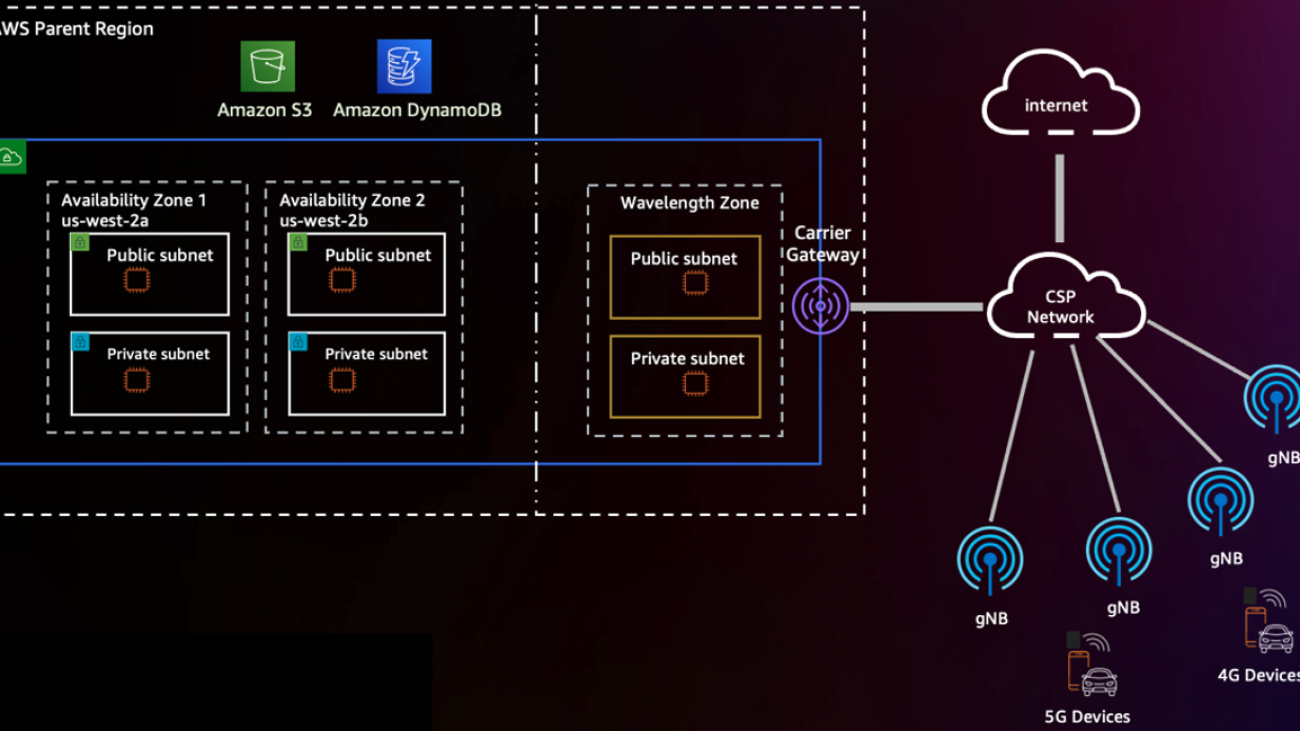
Solution overview
Across AWS’s rapidly expanding global infrastructure, AWS Wavelength brings the power of cloud compute and storage to the edge of 5G networks, unlocking more performant mobile experiences. With AWS Wavelength, you can extend your virtual private cloud (VPC) to Wavelength Zones corresponding to the telecommunications carrier’s network edge in 29 cities across the globe. The following diagram shows an example of this architecture.

You can opt in to the Wavelength Zones within a given Region via the AWS Management Console or the AWS Command Line Interface (AWS CLI). To learn more about deploying geo-distributed applications on AWS Wavelength, refer to Deploy geo-distributed Amazon EKS clusters on AWS Wavelength.
Building on the fundamentals discussed in this post, we look to ML at the edge as a sample workload with which to deploy to AWS Wavelength. As our sample workload, we deploy a pre-trained model from Amazon SageMaker JumpStart.
SageMaker is a fully managed ML service that allows developers to easily deploy ML models into their AWS environments. Although AWS offers a number of options for model training—from AWS Marketplace models and SageMaker built-in algorithms—there are a number of techniques to deploy open-source ML models.
JumpStart provides access to hundreds of built-in algorithms with pre-trained models that can be seamlessly deployed to SageMaker endpoints. From predictive maintenance and computer vision to autonomous driving and fraud detection, JumpStart supports a variety of popular use cases with one-click deployment on the console.
Because SageMaker is not natively supported in Wavelength Zones, we demonstrate how to extract the model artifacts from the Region and re-deploy to the edge. To do so, you use Amazon Elastic Kubernetes Service (Amazon EKS) clusters and node groups in Wavelength Zones, followed by creating a deployment manifest with the container image generated by JumpStart. The following diagram illustrates this architecture.

Prerequisites
To make this as easy as possible, ensure that your AWS account has Wavelength Zones enabled. Note that this integration is only available in us-east-1 and us-west-2, and you will be using us-east-1 for the duration of the demo.
To opt in to AWS Wavelength, complete the following steps:
- On the Amazon VPC console, choose Zones under Settings and choose US East (Verizon) / us-east-1-wl1.
- Choose Manage.
- Select Opted in.
- Choose Update zones.
Create AWS Wavelength infrastructure
Before we convert the local SageMaker model inference endpoint to a Kubernetes deployment, you can create an EKS cluster in a Wavelength Zone. To do so, deploy an Amazon EKS cluster with an AWS Wavelength node group. To learn more, you can visit this guide on the AWS Containers Blog or Verizon’s 5GEdgeTutorials repository for one such example.
Next, using an AWS Cloud9 environment or interactive development environment (IDE) of choice, download the requisite SageMaker packages and Docker Compose, a key dependency of JumpStart.
Create model artifacts using JumpStart
First, make sure that you have an AWS Identity and Access Management (IAM) execution role for SageMaker. To learn more, visit SageMaker Roles.
- Using this example, create a file called train_model.py that uses the SageMaker Software Development Kit (SDK) to retrieve a pre-built model (replace <your-sagemaker-execution-role> with the Amazon Resource Name (ARN) of your SageMaker execution role). In this file, you deploy a model locally using the
instance_typeattribute in themodel.deploy()function, which starts a Docker container within your IDE using all requisite model artifacts you defined:
- Next, set
infer_model_idto the ID of the SageMaker model that you would like to use.
For a complete list, refer to Built-in Algorithms with pre-trained Model Table. In our example, we use the Bidirectional Encoder Representations from Transformers (BERT) model, commonly used for natural language processing.
- Run the
train_model.pyscript to retrieve the JumpStart model artifacts and deploy the pre-trained model to your local machine:
Should this step succeed, your output may resemble the following:
In the output, you will see three artifacts in order: the base image for TensorFlow inference, the inference script that serves the model, and the artifacts containing the trained model. Although you could create a custom Docker image with these artifacts, another approach is to let SageMaker local mode create the Docker image for you. In the subsequent steps, we extract the container image running locally and deploy to Amazon Elastic Container Registry (Amazon ECR) as well as push the model artifact separately to Amazon Simple Storage Service (Amazon S3).
Convert local mode artifacts to remote Kubernetes deployment
Now that you have confirmed that SageMaker is working locally, let’s extract the deployment manifest from the running container. Complete the following steps:
Identify the location of the SageMaker local mode deployment manifest: To do so, search our root directory for any files named docker-compose.yaml.
docker_manifest=$( find /tmp/tmp* -name "docker-compose.yaml" -printf '%T+ %pn' | sort | tail -n 1 | cut -d' ' -f2-)
echo $docker_manifest
Identify the location of the SageMaker local mode model artifacts: Next, find the underlying volume mounted to the local SageMaker inference container, which will be used in each EKS worker node after we upload the artifact to Amazon s3.
model_local_volume = $(grep -A1 -w "volumes:" $docker_manifest | tail -n 1 | tr -d ' ' | awk -F: '{print $1}' | cut -c 2-)
# Returns something like: /tmp/tmpcr4bu_a7</p>
Create local copy of running SageMaker inference container: Next, we’ll find the currently running container image running our machine learning inference model and make a copy of the container locally. This will ensure we have our own copy of the container image to pull from Amazon ECR.
# Find container ID of running SageMaker Local container
mkdir sagemaker-container
container_id=$(docker ps --format "{{.ID}} {{.Image}}" | grep "tensorflow" | awk '{print $1}')
# Retrieve the files of the container locally
docker cp $my_container_id:/ sagemaker-container/
Before acting on the model_local_volume, which we’ll push to Amazon S3, push a copy of the running Docker image, now in the sagemaker-container directory, to Amazon Elastic Container Registry. Be sure to replace region, aws_account_id, docker_image_id and my-repository:tag or follow the Amazon ECR user guide. Also, be sure to take note of the final ECR Image URL (aws_account_id.dkr.ecr.region.amazonaws.com/my-repository:tag), which we will use in our EKS deployment.
Now that we have an ECR image corresponding to the inference endpoint, create a new Amazon S3 bucket and copy the SageMaker Local artifacts (model_local_volume) to this bucket. In parallel, create an Identity Access Management (IAM) that provides Amazon EC2 instances access to read objects within the bucket. Be sure to replace <unique-bucket-name> with a globally unique name for your Amazon S3 bucket.
Next, to ensure that each EC2 instance pulls a copy of the model artifact on launch, edit the user data for your EKS worker nodes. In your user data script, ensure that each node retrieves the model artifacts using the the S3 API at launch. Be sure to replace <unique-bucket-name> with a globally unique name for your Amazon S3 bucket. Given that the node’s user data will also include the EKS bootstrap script, the complete user data may look something like this.
Now, you can inspect the existing docker manifest it and translate it to Kubernetes-friendly manifest files using Kompose, a well-known conversion tool. Note: if you get a version compatibility error, change the version attribute in line 27 of docker-compose.yml to “2”.
After running Kompose, you’ll see four new files: a Deployment object, Service object, PersistentVolumeClaim object, and NetworkPolicy object. You now have everything you need to begin your foray into Kubernetes at the edge!
Deploy SageMaker model artifacts
Make sure you have kubectl and aws-iam-authenticator downloaded to your AWS Cloud9 IDE. If not, follow the installation guides:
Now, complete the following steps:
Modify the service/algo-1-ow3nv object to switch the service type from ClusterIP to NodePort. In our example, we have selected port 30,007 as our NodePort:
Next, you must allow the NodePort in the security group for your node. To do so, retrieve the security groupID and allow-list the NodePort:
Next, modify the algo-1-ow3nv-deployment.yaml manifest to mount the /tmp/model hostPath directory to the container. Replace <your-ecr-image> with the ECR image you created earlier:
With the manifest files you created from Kompose, use kubectl to apply the configs to your cluster:
Connect to the 5G edge model
To connect to your model, complete the following steps:
On the Amazon EC2 console, retrieve the carrier IP of the EKS worker node or use the AWS CLI to query the carrier IP address directly:
Now, with the carrier IP address extracted, you can connect to the model directly using the NodePort. Create a file called invoke.py to invoke the BERT model directly by providing a text-based input that will be run against a sentiment-analyzer to determine whether the tone was positive or negative:
Your output should resemble the following:
Clean up
To destroy all application resources created, delete the AWS Wavelength worker nodes, the EKS control plane, and all the resources created within the VPC. Additionally, delete the ECR repo used to host the container image, the S3 buckets used to host the SageMaker model artifacts and the sagemaker-demo-app-s3 IAM policy.
Conclusion
In this post, we demonstrated a novel approach to deploying SageMaker models to the network edge using Amazon EKS and AWS Wavelength. To learn about Amazon EKS best practices on AWS Wavelength, refer to Deploy geo-distributed Amazon EKS clusters on AWS Wavelength. Additionally, to learn more about Jumpstart, visit the Amazon SageMaker JumpStart Developer Guide or the JumpStart Available Model Table.
About the Authors
 Robert Belson is a Developer Advocate in the AWS Worldwide Telecom Business Unit, specializing in AWS Edge Computing. He focuses on working with the developer community and large enterprise customers to solve their business challenges using automation, hybrid networking and the edge cloud.
 Mohammed Al-Mehdar is a Senior Solutions Architect in the Worldwide Telecom Business Unit at AWS. His main focus is to help enable customers to build and deploy Telco and Enterprise IT workloads on AWS. Prior to joining AWS, Mohammed has been working in the Telco industry for over 13 years and brings a wealth of experience in the areas of LTE Packet Core, 5G, IMS and WebRTC. Mohammed holds a bachelor’s degree in Telecommunications Engineering from Concordia University.
 Evan Kravitz is a software engineer at Amazon Web Services, working on SageMaker JumpStart. He enjoys cooking and going on runs in New York City.
 Justin St. Arnauld is an Associate Director – Solution Architects at Verizon for the Public Sector with over 15 years of experience in the IT industry. He is a passionate advocate for the power of edge computing and 5G networks and is an expert in developing innovative technology solutions that leverage these technologies. Justin is particularly enthusiastic about the capabilities offered by Amazon Web Services (AWS) in delivering cutting-edge solutions for his clients. In his free time, Justin enjoys keeping up-to-date with the latest technology trends and sharing his knowledge and insights with others in the industry.

Directing ML toward natural hazard mitigation through collaboration
Floods are the most common type of natural disaster, affecting more than 250 million people globally each year. As part of Google’s Crisis Response and our efforts to address the climate crisis, we are using machine learning (ML) models for Flood Forecasting to alert people in areas that are impacted before disaster strikes.
Collaboration between researchers in the industry and academia is essential for accelerating progress towards mutual goals in ML-related research. Indeed, Google’s current ML-based flood forecasting approach was developed in collaboration with researchers (1, 2) at the Johannes Kepler University in Vienna, Austria, the University of Alabama, and the Hebrew University of Jerusalem, among others.
Today we discuss our recent Machine Learning Meets Flood Forecasting Workshop, which highlights efforts to bring together researchers from Google and other universities and organizations to advance our understanding of flood behavior and prediction, and build more robust solutions for early detection and warning. We also discuss the Caravan project, which is helping to create an open-source repository for global streamflow data, and is itself an example of a collaboration that developed from the previous Flood Forecasting Meets Machine Learning Workshop.
2023 Machine Learning Meets Flood Forecasting Workshop
The fourth annual Google Machine Learning Meets Flood Forecasting Workshop was held in January. This 2-day virtual workshop hosted over 100 participants from 32 universities, 20 governmental and non-governmental agencies, and 11 private companies. This forum provided an opportunity for hydrologists, computer scientists, and aid workers to discuss challenges and efforts toward improving global flood forecasts, to keep up with state-of-the-art technology advances, and to integrate domain knowledge into ML-based forecasting approaches.
The event included talks from six invited speakers, a series of small-group discussion sessions focused on hydrological modeling, inundation mapping, and hazard alerting–related topics, as well as a presentation by Google on the FloodHub, which provides free, public access to Google’s flood forecasts, up to 7 days in advance.
 |
Invited speakers at the workshop included:
- Chaopeng Shen (Associate Professor at Pennsylvania State University) talked about recent research related to integrating physically-based hydrology models with ML.
- Beth Tellman (Assistant Professor at the University of Arizona & Chief Science Officer at Floodbase) gave an overview of recent efforts to map inundation in the United States using ML with input from NOAA’s US National Water Model.
- Frederik Kratzert (Research Scientist at Google) provided an overview of the Caravan project (below).
- Maulik Jagnani (Assistant Professor at the University of Colorado Denver) discussed a series of studies that measured how communities in India received and acted on perceived flood alerts from Google’s flood forecasting system.
- Shruti Verma (UX Researcher with the Flood Forecasting team at Google) discussed how UX research plays a role in understanding the people and populations who live in flood-prone regions around the world.
- Justin Sheffield (Professor and Head of the School of Geography and Environmental Science at the University of Southampton) talked about an operational forecasting system called the African Flood and Drought Monitor (AFDM).
The presentations can be viewed on YouTube:
2023 Flood Forecasting Meets Machine Learning Talks Day 1
2023 Flood Forecasting Meets Machine Learning Talks Day 2
Some of the top challenges highlighted during the workshop were related to the integration of physical and hydrological science with ML to help build trust and reliability; filling gaps in observations of inundated areas with models and satellite data; measuring the skill and reliability of flood warning systems; and improving the communication of flood warnings to diverse, global populations. In addition, participants stressed that addressing these and other challenges will require collaboration between a number of different organizations and scientific disciplines.
The Caravan project
One of the main challenges in conducting successful ML research and creating advanced tools for flood forecasting is the need for large amounts of data for computationally expensive training and evaluation. Today, many countries and organizations collect streamflow data (typically either water levels or flow rates), but it is not standardized or held in a central repository, which makes it difficult for researchers to access.
During the 2019 Machine Learning Meets Flood Forecasting Workshop, a group of researchers identified the need for an open source, global streamflow data repository, and developed ideas around leveraging free computational resources from Google Earth Engine to address the flood forecasting community’s challenge of data collection and accessibility. Following two years of collaborative work between researchers from Google, the school of Geography at the University of Exeter, the Institute for Machine Learning at Johannes Kepler University, and the Institute for Atmospheric and Climate Science at ETH Zurich, the Caravan project was created.
In “Caravan – A global community dataset for large-sample hydrology”, published in Nature Scientific Data, we describe the project in more detail. Based on a global dataset for the development and training of hydrological models (see figure below), Caravan provides open-source Python scripts that leverage essential weather and geographical data that was previously made public on Google Earth Engine to match streamflow data that users upload to the repository. This repository originally contained data from more than 13,000 watersheds in Central Europe, Brazil, Chile, Australia, the United States, Canada, and Mexico. It has further benefited from community contributions from the Geological Survey of Denmark and Greenland that includes streamflow data from most of the watersheds in Denmark. The goal is to continue to develop and grow this repository to enable researchers to access most of the world’s streamflow data. For more information regarding contributing to the Caravan dataset, reach out to caravan@google.com.
 |
 |
| Locations of the 13,000 streamflow gauges in the Caravan dataset and the distribution of those gauges in GEnS global climate zones. |
The path forward
Google plans to continue to host these workshops to help broaden and deepen collaboration between industry and academia in the development of environmental AI models. We are looking forward to seeing what advances might come out of the most recent workshop. Hydrologists and researchers interested in participating in future workshops are encouraged to contact flood-forecasting-meets-ml@google.com.
Celebrate PyTorch* 2.0 with New Performance Features for AI Developers
Congratulations to the PyTorch Foundation for its release of PyTorch* 2.0! In this blog, I discuss the four features for which Intel made significant contributions to PyTorch 2.0:
- TorchInductor
- GNN
- INT8 Inference Optimization
- oneDNN Graph API
We at Intel are delighted to be part of the PyTorch community and appreciate the collaboration with and feedback from our colleagues at Meta as we co-developed these features.
Let’s get started.
1. TorchInductor CPU FP32 Inference Optimized
As part of the PyTorch 2.0 compilation stack, TorchInductor CPU backend optimization brings notable performance improvements via graph compilation over the PyTorch eager mode.
The TorchInductor CPU backend is sped up by leveraging the technologies from the Intel® Extension for PyTorch for Conv/GEMM ops with post-op fusion and weight prepacking, and PyTorch ATen CPU kernels for memory-bound ops with explicit vectorization on top of OpenMP*-based thread parallelization.
With these optimizations on top of the powerful loop fusions in TorchInductor codegen, we achieved up to a 1.7x FP32 inference performance boost over three representative deep learning benchmarks: TorchBench, HuggingFace, and timm1. Training and low-precision support are under development.
See the Improvements
The performance improvements on various backends are tracked on this TouchInductor CPU Performance Dashboard.
Improve Graph Neural Network (GNN) in PyG for Inference and Training Performance on CPU
GNN is a powerful tool to analyze graph structure data. This feature is designed to improve GNN inference and training performance on Intel® CPUs, including the new 4th Gen Intel® Xeon® Scalable processors.
PyTorch Geometric (PyG) is a very popular library built upon PyTorch to perform GNN workflows. Currently on CPU, GNN models of PyG run slowly due to the lack of GNN-related sparse matrix multiplication operations (i.e., SpMM_reduce) and the lack of several critical kernel-level optimizations (scatter/gather, etc.) tuned for GNN compute.
To address this, optimizations are provided for message passing between adjacent neural network nodes:
- scatter_reduce: performance hotspot in message-passing when the edge index is stored in coordinate format (COO).
- gather: backward computation of scatter_reduce, specially tuned for the GNN compute when the index is an expanded tensor.
- torch.sparse.mm with reduce flag: performance hotspot in message-passing when the edge index is stored in compressed sparse row (CSR). Supported reduce flag for: sum, mean, amax, amin.
End-to-end performance benchmark results for both inference and training on 3rd Gen Intel® Xeon® Scalable processors 8380 platform and on 4th Gen 8480+ platform are discussed in Accelerating PyG on Intel CPUs.
Optimize int8 Inference with Unified Quantization Backend for x86 CPU Platforms
The new X86 quantization backend is a combination of FBGEMM (Facebook General Matrix-Matrix Multiplication) and oneAPI Deep Neural Network Library (oneDNN) backends and replaces FBGEMM as the default quantization backend for x86 platforms. The result: better end-to-end int8 inference performance than FBGEMM.
Users access the x86 quantization backend by default for x86 platforms, and the selection between different kernels is automatically done behind the scenes. The rules of selection are based on prior performance testing data done by Intel during feature development. Thus, the x86 backend replaces FBGEMM and may offer better performance, depending on the use case.
The selection rules are:
- On platforms without VNNI (e.g., Intel® Core™ i7 processors), FBGEMM is always used.
- On platforms with VNNI (e.g., 2nd-4th Gen Intel® Xeon® Scalable processors and future platforms):
- For linear, FBGEMM is always used.
- For convolution layers, FBGEMM is used for depth-wise convolution whose layers > 100; otherwise, oneDNN is used.
Note that as the kernels continue to evolve.
The selection rules above are subject to change to achieve better performance. Performance metrics for through-put speed-up ratios of unified x86 backend vs. pure FBGEMM are discussed in [RFC] Unified quantization backend for x86 CPU platforms #83888.
Leverage oneDNN Graph API to Accelerate Inference on CPU
oneDNN Graph API extends oneDNN with a flexible graph API to maximize the optimization opportunity for generating efficient code on Intel® AI hardware. It automatically identifies the graph partitions to be accelerated via fusion. The fusion patterns focus on fusing compute-intensive operations such as convolution, matmul, and their neighbor operations for both inference and training use cases.
Currently, BFloat16 and Float32 datatypes are supported and only inference workloads can be optimized. BF16 is only optimized on machines with Intel® Advanced Vector Extensions 512 (Intel® AVX-512) BF16 support.
Few or no modifications are needed in PyTorch to support newer oneDNN Graph fusions/optimized kernels. To use oneDNN Graph, users can:
- Either use the API torch.jit.enable_onednn_fusion(True) before JIT tracing a model, OR …
- Use its context manager, viz. with torch.jit.fuser(“fuser3”).
- For accelerating BFloat16 inference, we rely on eager-mode AMP (Automatic Mixed Precision) support in PyTorch and disable JIT mode’s AMP.
See the PyTorch performance tuning guide.
Next Steps
Get the Software
Try out PyTorch 2.0 and realize the performance benefits for yourself from these Intel-contributed features.
We encourage you to check out Intel’s other AI Tools and Framework optimizations and learn about the open, standards-based oneAPI multiarchitecture, multivendor programming model that forms the foundation of Intel’s AI software portfolio.
For more details about 4th Gen Intel Xeon Scalable processor, visit AI Platform where you can learn about how Intel is empowering developers to run high-performance, efficient end-to-end AI pipelines.