DeepMind and the Brain team from Google Research will join forces to accelerate progress towards a world in which AI helps solve the biggest challenges facing humanity.Read More

DeepMind and the Brain team from Google Research will join forces to accelerate progress towards a world in which AI helps solve the biggest challenges facing humanity.Read More

DeepMind and the Brain team from Google Research will join forces to accelerate progress towards a world in which AI helps solve the biggest challenges facing humanity.Read More
DeepMind and the Brain team from Google Research will join forces to accelerate progress towards a world in which AI helps solve the biggest challenges facing humanity.Read More

DeepMind and the Brain team from Google Research will join forces to accelerate progress towards a world in which AI helps solve the biggest challenges facing humanity.Read More
The ability to effectively handle and process enormous amounts of documents has become essential for enterprises in the modern world. Due to the continuous influx of information that all enterprises deal with, manually classifying documents is no longer a viable option. Document classification models can automate the procedure and help organizations save time and resources. Traditional categorization techniques, such as manual processing and keyword-based searches, become less efficient and more time-consuming as the volume of documents increases. This inefficiency causes lower productivity and higher operating expenses. Additionally, it can prevent crucial information from being accessible when needed, which could lead to a poor customer experience and impact decision-making. At AWS re:Invent 2022, Amazon Comprehend, a natural language processing (NLP) service that uses machine learning (ML) to discover insights from text, launched support for native document types. This new feature gave you the ability to classify documents in native formats (PDF, TIFF, JPG, PNG, DOCX) using Amazon Comprehend.
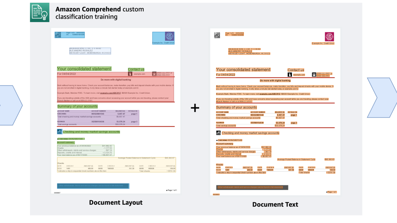
Today, we are excited to announce that Amazon Comprehend now supports custom classification model training with documents like PDF, Word, and image formats. You can now train bespoke document classification models on native documents that support layout in addition to text, increasing the accuracy of the results.
In this post, we provide an overview of how you can get started with training an Amazon Comprehend custom document classification model.
The capacity to understand the relative placements of objects within a defined space is referred to as layout awareness. In this case, it aids the model in understanding how headers, subheadings, tables, and graphics relate to one another inside a document. The model can more effectively categorize a document based on its content when it’s aware of the structure and layout of the text.
In this post, we walk through the data preparation steps involved, demonstrate the model training process, and discuss the benefits of using the new custom document classification model in Amazon Comprehend. As a best practice, you should consider the following points before you begin training the custom document classification model.
Identify the various types of documents they you may need to classify, along with the different classes or categories to support your use case. Determine the suitable classification structure or taxonomy after evaluating the amount and types of documents that need to be categorized. Document types may vary from PDF, Word, images, and so on. Ensure you have authorized access to a diverse set of labeled documents either via a document management system or other storage mechanisms.
Ensure that the document files you intend to use for model training aren’t encrypted or locked—for example, make sure that your PDF files aren’t encrypted and locked with a password. You must decrypt such files before you can use them for training purposes. Label a sample of your documents with the appropriate categories or labels (classes). Determine whether single-label classification (multi-class mode) or multi-label classification is appropriate for your use case. Multi-class mode associates only a single class with each document, whereas multi-label mode associates one or more class with a document.
Use the labeled dataset to train the model so it can learn to classify new documents accurately and evaluate how the newly trained model version performs by understanding the model metrics. To understand the metrics provided by Amazon Comprehend post-model training, refer to Custom classifier metrics. After the training process is complete, you can begin classifying documents asynchronously or in real time. We walk through how to train a custom classification model in the following sections.
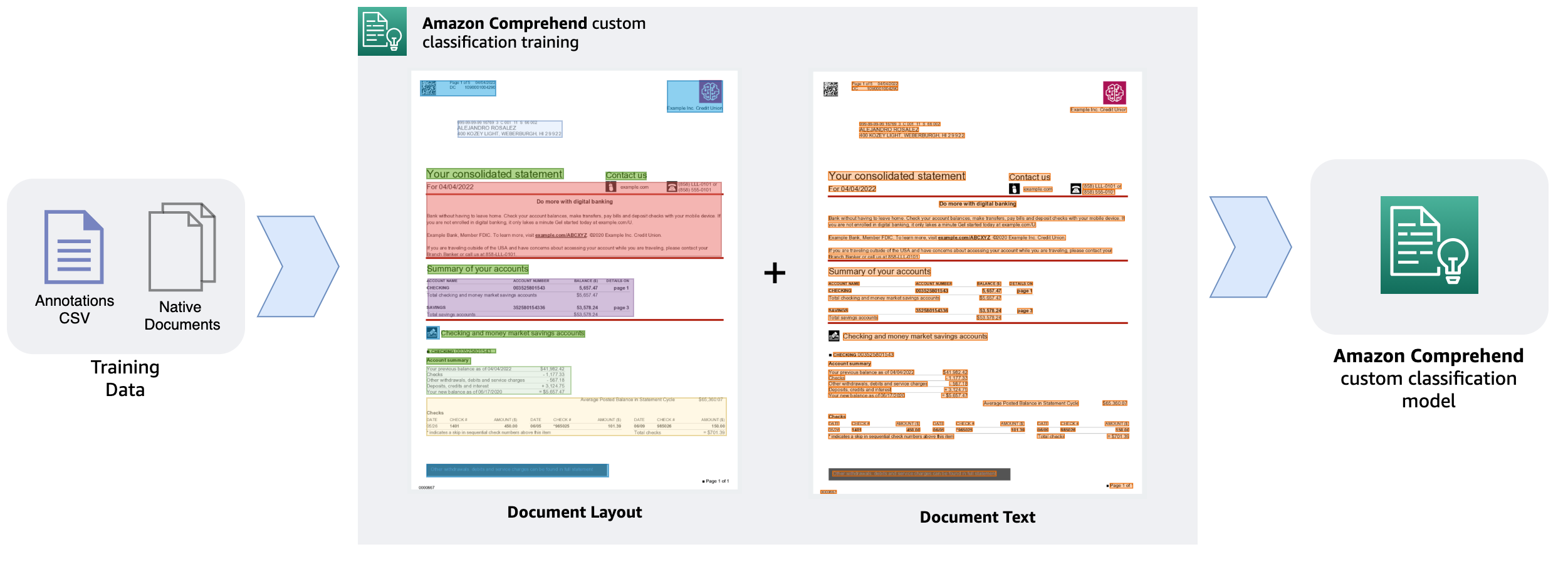
Before we train our custom classification model, we need to prepare the training data. Training data is comprised of a set of labeled documents, which can be pre-identified documents from a document repository that you already have access to. For our example, we trained a custom classification model with a few different document types that are typically found in a health insurance claim adjudication process: patient discharge summary, invoices, receipts, and so on. We also need to prepare an annotations file in CSV format. Following is an example of an annotations file CSV data required for the training:
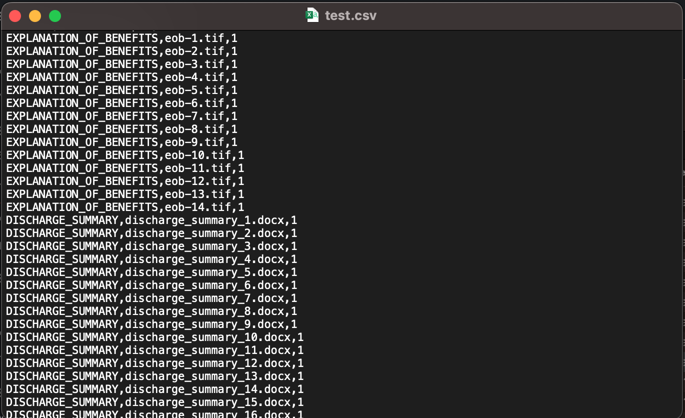
The annotations CSV file must contain three columns. The first column contains the desired class (label) for the document, the second column is the document name (file name), and the last column is the page number of the document that you want to include in the training dataset. Because the training process supports native multi-page PDF and DOCX files, you must specify the page number in case the document is a multi-page document. If you want to include all pages of a multi-page document in the training dataset, you must specify each page as a separate line in the CSV annotations file. For example, in the preceding annotations file, invoice-1.pdf is a two-page document, and we want to include both pages in the classification dataset. Because files like PDF, PNG, and TIFF are image formats, the page number (third column) value must always be 1. If your dataset contains multi-frame (multi-page) TIF files, you must split them into separate TIF files in order to use them in the training process.
We prepared an annotations file called test.csv with the appropriate data to train a custom classification model. For each sample document, the CSV file contains the class that document belongs to, the location of the document in Amazon Simple Storage Service (Amazon S3), such as path/to/prefix/document.pdf, and the page number (if applicable). Because most of our documents are either single-page DOCX, PDF files, or TIF, JPG, or PNG files, the page number assigned is 1. Because our annotations CSV and sample documents are all under the same Amazon S3 prefix, we don’t need to explicitly specify the prefix in the second column. We also prepare at least 10 document samples or more for each class, and we used a mix of JPG, PNG, DOCX, PDF, and TIF files for training the model. Note that it’s usually recommended to have a diverse set of sample documents for model training to avoid overfitting of the model, which impacts its ability to recognize new documents. It’s also recommended that the number of samples per class is balanced, although it’s not required to have an exact same number of samples per class. Next, we upload the test.csv annotations file and all the documents into Amazon S3. The following image shows part of our annotations CSV file.
Now that we have the annotations file and all our sample documents ready, we set up a custom classification model and train it. Before you begin setting up custom classification model training, make sure that the annotations CSV and sample documents exist in an Amazon S3 location.


This tells Amazon Comprehend that you intend to use native document types to train the model instead of serialized text.
This mode tells the classifier that we intend to classify documents into a single class. If you need to train a model with multi-label mode, meaning a document may belong to one or more than one class, you must set up the annotations file appropriately by specifying the classes of the document separated by a special character in the annotations CSV file. In that case, you would select the Using multi-label mode option.

This is optional, but it’s a good practice to provide an output location because Amazon Comprehend will generate the post-model training evaluation metrics in this location. This data is useful to evaluate model performance, iterate, and improve the accuracy of your model.

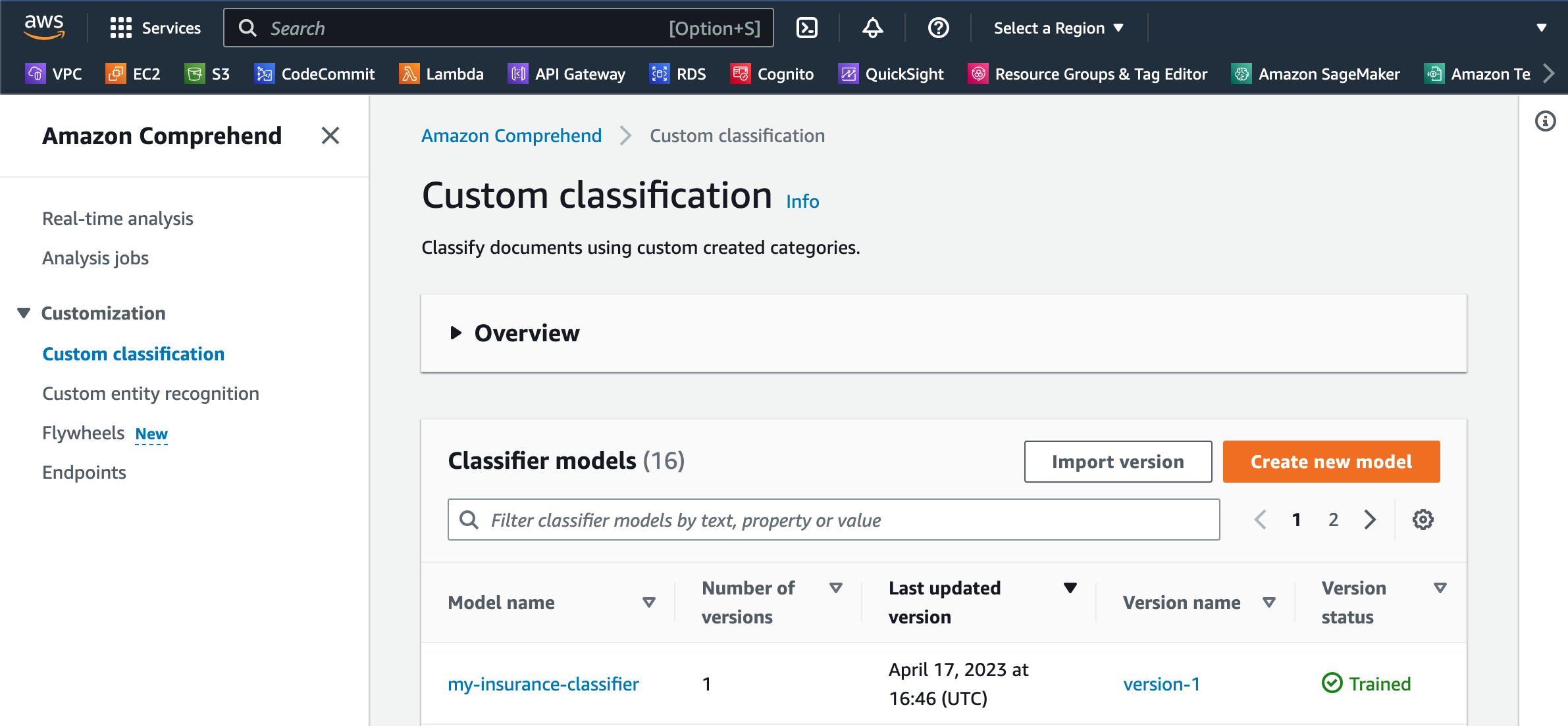
The model may take several minutes to train, depending on the number of classes and the dataset size. You can review the training status on the Custom classification page. The training process will display a Submitted status right after the training process starts and will change to Training status when the training process begins. After your model is trained, the Version status will change to Trained. If Amazon Comprehend finds inconsistencies in your training data, the status will show In error along with an alert that shows the appropriate error message so that you can take corrective action and restart the training process with the corrected data.
In this post, we demonstrated the steps to train a custom classifier model using the Amazon Comprehend console. You can also use the AWS SDK in any language (for example, Boto3 for Python) or the AWS Command Line Interface (AWS CLI) to initiate a custom classification model training. With either the SDK or AWS CLI, you can use the CreateDocumentClassifier API to initiate the model training, and subsequently use the DescribeDocumentClassifier API to check the status of the model.
After the model is trained, you can perform either real-time analysis or asynchronous (batch) analysis jobs on new documents. To perform real-time classification on documents, you must deploy an Amazon Comprehend real-time endpoint with the trained custom classification model. Real-time endpoints are best suited for use cases that require low-latency, real-time inference results, whereas for classifying a large set of documents, an asynchronous analysis job is more appropriate. To learn how you can perform asynchronous inference on new documents using a trained classification model, refer to Introducing one-step classification and entity recognition with Amazon Comprehend for intelligent document processing.
The new classifier model offers a number of improvements. It’s not only easier to train the new model, but you can also train a new model with just a few samples for each class. Additionally, you no longer have to extract serialized plain text out of scanned or digital documents such as images or PDFs to prepare the training dataset. The following are some additional noteworthy improvements that you can expect from the new classification model:
The new Amazon Comprehend document classification model, which incorporates layout awareness, is a game-changer for businesses dealing with large volumes of documents. By understanding the structure and layout of documents, this model offers improved classification accuracy and efficiency. Implementing a robust and accurate document classification solution using a layout-aware model can help your business save time, reduce operational costs, and enhance decision-making processes.
As a next step, we encourage you to try the new Amazon Comprehend custom classification model via the Amazon Comprehend console. We also recommend revisiting our custom classification model improvement announcements from last year and visit the GitHub repository for code samples.
 Anjan Biswas is a Senior AI Services Solutions Architect with a focus on AI/ML and Data Analytics. Anjan is part of the world-wide AI services team and works with customers to help them understand and develop solutions to business problems with AI and ML. Anjan has over 14 years of experience working with global supply chain, manufacturing, and retail organizations, and is actively helping customers get started and scale on AWS AI services.
 Godwin Sahayaraj Vincent is an Enterprise Solutions Architect at AWS who is passionate about Machine Learning and providing guidance to customers to design, deploy and manage their AWS workloads and architectures. In his spare time, he loves to play cricket with his friends and tennis with his three kids.
 Wrick Talukdar is a Senior Architect with the Amazon Comprehend Service team. He works with AWS customers to help them adopt machine learning on a large scale. Outside of work, he enjoys reading and photography.

Google sees AI as a foundational and transformational technology, with recent advances in generative AI technologies, such as LaMDA, PaLM, Imagen, Parti, MusicLM, and similar machine learning (ML) models, some of which are now being incorporated into our products. This transformative potential requires us to be responsible not only in how we advance our technology, but also in how we envision which technologies to build, and how we assess the social impact AI and ML-enabled technologies have on the world. This endeavor necessitates fundamental and applied research with an interdisciplinary lens that engages with — and accounts for — the social, cultural, economic, and other contextual dimensions that shape the development and deployment of AI systems. We must also understand the range of possible impacts that ongoing use of such technologies may have on vulnerable communities and broader social systems.
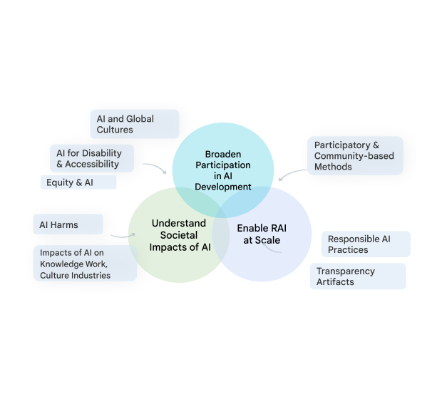
Our team, Technology, AI, Society, and Culture (TASC), is addressing this critical need. Research on the societal impacts of AI is complex and multi-faceted; no one disciplinary or methodological perspective can alone provide the diverse insights needed to grapple with the social and cultural implications of ML technologies. TASC thus leverages the strengths of an interdisciplinary team, with backgrounds ranging from computer science to social science, digital media and urban science. We use a multi-method approach with qualitative, quantitative, and mixed methods to critically examine and shape the social and technical processes that underpin and surround AI technologies. We focus on participatory, culturally-inclusive, and intersectional equity-oriented research that brings to the foreground impacted communities. Our work advances Responsible AI (RAI) in areas such as computer vision, natural language processing, health, and general purpose ML models and applications. Below, we share examples of our approach to Responsible AI and where we are headed in 2023.
 |
| A visual diagram of the various social, technical, and equity-oriented research areas that TASC studies to progress Responsible AI in a way that respects the complex relationships between AI and society. |
One of our key areas of research is the advancement of methods to make generative AI technologies more inclusive of and valuable to people globally, through community-engaged, and culturally-inclusive approaches. Toward this aim, we see communities as experts in their context, recognizing their deep knowledge of how technologies can and should impact their own lives. Our research champions the importance of embedding cross-cultural considerations throughout the ML development pipeline. Community engagement enables us to shift how we incorporate knowledge of what’s most important throughout this pipeline, from dataset curation to evaluation. This also enables us to understand and account for the ways in which technologies fail and how specific communities might experience harm. Based on this understanding we have created responsible AI evaluation strategies that are effective in recognizing and mitigating biases along multiple dimensions.
Our work in this area is vital to ensuring that Google’s technologies are safe for, work for, and are useful to a diverse set of stakeholders around the world. For example, our research on user attitudes towards AI, responsible interaction design, and fairness evaluations with a focus on the global south demonstrated the cross-cultural differences in the impact of AI and contributed resources that enable culturally-situated evaluations. We are also building cross-disciplinary research communities to examine the relationship between AI, culture, and society, through our recent and upcoming workshops on Cultures in AI/AI in Culture, Ethical Considerations in Creative Applications of Computer Vision, and Cross-Cultural Considerations in NLP.
Our recent research has also sought out perspectives of particular communities who are known to be less represented in ML development and applications. For example, we have investigated gender bias, both in natural language and in contexts such as gender-inclusive health, drawing on our research to develop more accurate evaluations of bias so that anyone developing these technologies can identify and mitigate harms for people with queer and non-binary identities.
We work to enable RAI at scale, by establishing industry-wide best practices for RAI across the development pipeline, and ensuring our technologies verifiably incorporate that best practice by default. This applied research includes responsible data production and analysis for ML development, and systematically advancing tools and practices that support practitioners in meeting key RAI goals like transparency, fairness, and accountability. Extending earlier work on Data Cards, Model Cards and the Model Card Toolkit, we released the Data Cards Playbook, providing developers with methods and tools to document appropriate uses and essential facts related to a dataset. Because ML models are often trained and evaluated on human-annotated data, we also advance human-centric research on data annotation. We have developed frameworks to document annotation processes and methods to account for rater disagreement and rater diversity. These methods enable ML practitioners to better ensure diversity in annotation of datasets used to train models, by identifying current barriers and re-envisioning data work practices.
We are now working to further broaden participation in ML model development, through approaches that embed a diversity of cultural contexts and voices into technology design, development, and impact assessment to ensure that AI achieves societal goals. We are also redefining responsible practices that can handle the scale at which ML technologies operate in today’s world. For example, we are developing frameworks and structures that can enable community engagement within industry AI research and development, including community-centered evaluation frameworks, benchmarks, and dataset curation and sharing.
In particular, we are furthering our prior work on understanding how NLP language models may perpetuate bias against people with disabilities, extending this research to address other marginalized communities and cultures and including image, video, and other multimodal models. Such models may contain tropes and stereotypes about particular groups or may erase the experiences of specific individuals or communities. Our efforts to identify sources of bias within ML models will lead to better detection of these representational harms and will support the creation of more fair and inclusive systems.
TASC is about studying all the touchpoints between AI and people — from individuals and communities, to cultures and society. For AI to be culturally-inclusive, equitable, accessible, and reflective of the needs of impacted communities, we must take on these challenges with inter- and multidisciplinary research that centers the needs of impacted communities. Our research studies will continue to explore the interactions between society and AI, furthering the discovery of new ways to develop and evaluate AI in order for us to develop more robust and culturally-situated AI technologies.
We would like to thank everyone on the team that contributed to this blog post. In alphabetical order by last name: Cynthia Bennett, Eric Corbett, Aida Mostafazadeh Davani, Emily Denton, Sunipa Dev, Fernando Diaz, Mark Díaz, Shaun Kane, Shivani Kapania, Michael Madaio, Vinodkumar Prabhakaran, Rida Qadri, Renee Shelby, Ding Wang, and Andrew Zaldivar. Also, we would like to thank Toju Duke and Marian Croak for their valuable feedback and suggestions.
Businesses are increasingly using machine learning (ML) to make near-real-time decisions, such as placing an ad, assigning a driver, recommending a product, or even dynamically pricing products and services. ML models make predictions given a set of input data known as features, and data scientists easily spend more than 60% of their time designing and building these features. Furthermore, highly accurate predictions depend on timely access to feature values that change quickly over time, adding even more complexity to the job of building a highly available and accurate solution. For example, a model for a ride-sharing app can choose the best price for a ride from the airport, but only if it knows the number of ride requests received in the past 10 minutes and the number of passengers projected to land in the next 10 minutes. A routing model in a call center app can pick the best available agent for an incoming call, but it’s only effective if it knows the customer’s latest web session clicks.
Although the business value of near-real-time ML predictions is enormous, the architecture required to deliver them reliably, securely, and with good performance is complicated. Solutions need high-throughput updates and low-latency retrieval of the most recent feature values in milliseconds, something most data scientists aren’t prepared to deliver. As a result, some enterprises have spent millions of dollars inventing their own proprietary infrastructure for feature management. Other firms have limited their ML applications to simpler patterns like batch scoring until ML vendors provide more comprehensive off-the-shelf solutions for online feature stores.
To address these challenges, Amazon SageMaker Feature Store provides a fully managed central repository for ML features, making it easy to securely store and retrieve features without having to build and maintain your own infrastructure. Feature Store lets you define groups of features, use batch ingestion and streaming ingestion, retrieve the latest feature values with single-digit millisecond latency for highly accurate online predictions, and extract point-in-time correct datasets for training. Instead of building and maintaining these infrastructure capabilities, you get a fully managed service that scales as your data grows, enables sharing features across teams, and lets your data scientists focus on building great ML models aimed at game-changing business use cases. Teams can now deliver robust features once and reuse them many times in a variety of models that may be built by different teams.
This post walks through a complete example of how you can couple streaming feature engineering with Feature Store to make ML-backed decisions in near-real time. We show a credit card fraud detection use case that updates aggregate features from a live stream of transactions and uses low-latency feature retrievals to help detect fraudulent transactions. Try it out for yourself by visiting our GitHub repo.
Stolen credit card numbers can be bought in bulk on the dark web from previous leaks or hacks of organizations that store this sensitive data. Fraudsters buy these card lists and attempt to make as many transactions as possible with the stolen numbers until the card is blocked. These fraud attacks typically happen in a short time frame, and this can be easily spotted in historical transactions because the velocity of transactions during the attack differs significantly from the cardholder’s usual spending pattern.
The following table shows a sequence of transactions from one credit card where the cardholder first has a genuine spending pattern, and then experiences a fraud attack starting on November 4.
| cc_num | trans_time | amount | fraud_label |
| …1248 | Nov-01 14:50:01 | 10.15 | 0 |
| … 1248 | Nov-02 12:14:31 | 32.45 | 0 |
| … 1248 | Nov-02 16:23:12 | 3.12 | 0 |
| … 1248 | Nov-04 02:12:10 | 1.01 | 1 |
| … 1248 | Nov-04 02:13:34 | 22.55 | 1 |
| … 1248 | Nov-04 02:14:05 | 90.55 | 1 |
| … 1248 | Nov-04 02:15:10 | 60.75 | 1 |
| … 1248 | Nov-04 13:30:55 | 12.75 | 0 |
For this post, we train an ML model to spot this kind of behavior by engineering features that describe an individual card’s spending pattern, such as the number of transactions or the average transaction amount from that card in a certain time window. This model protects cardholders from fraud at the point of sale by detecting and blocking suspicious transactions before the payment can complete. The model makes predictions in a low-latency, real-time context and relies on receiving up-to-the-minute feature calculations so it can respond to an ongoing fraud attack. In a real-world scenario, features related to cardholder spending patterns would only form part of the model’s feature set, and we can include information about the merchant, the cardholder, the device used to make the payment, and any other data that may be relevant to detecting fraud.
Because our use case relies on profiling an individual card’s spending patterns, it’s crucial that we can identify credit cards in a transaction stream. Most publicly available fraud detection datasets don’t provide this information, so we use the Python Faker library to generate a set of transactions covering a 5-month period. This dataset contains 5.4 million transactions spread across 10,000 unique (and fake) credit card numbers, and is intentionally imbalanced to match the reality of credit card fraud (only 0.25% of the transactions are fraudulent). We vary the number of transactions per day per card, as well as the transaction amounts. See our GitHub repo for more details.
We want our fraud detection model to classify credit card transactions by noticing a burst of recent transactions that differs significantly from the cardholder’s usual spending pattern. Sounds simple enough, but how do we build it?
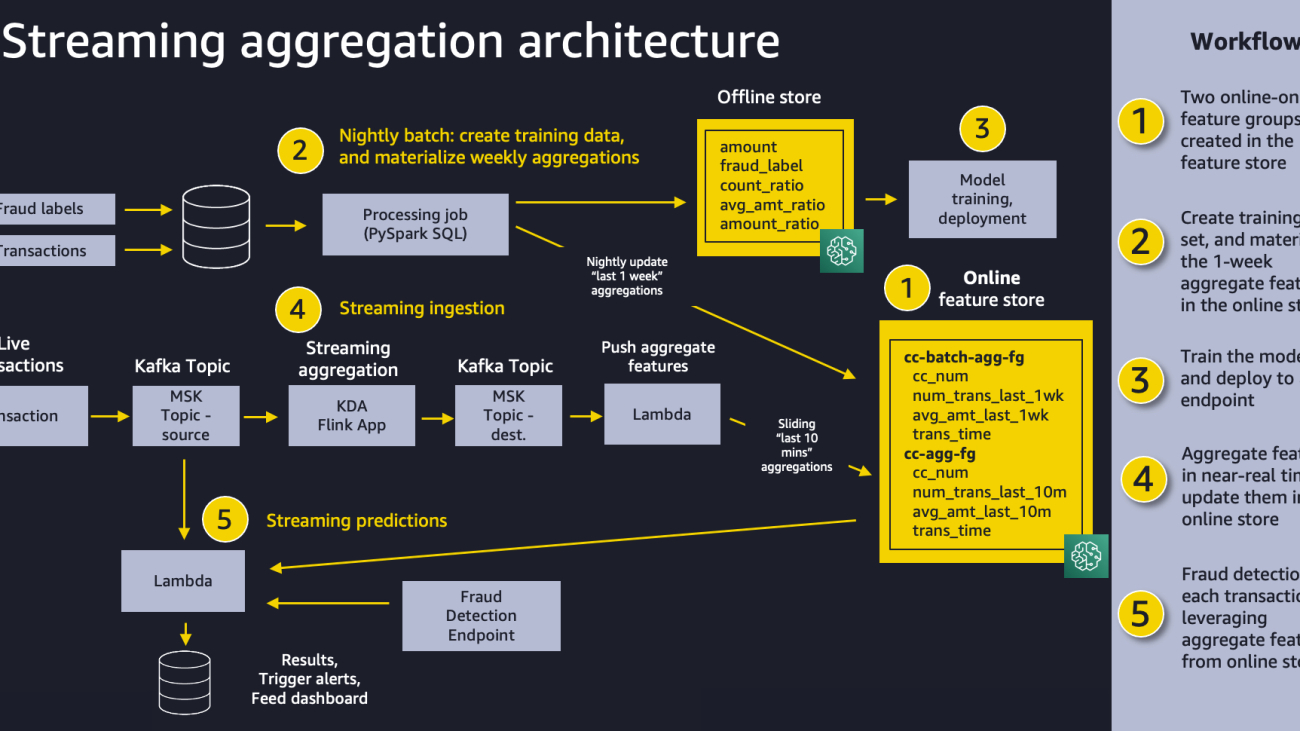
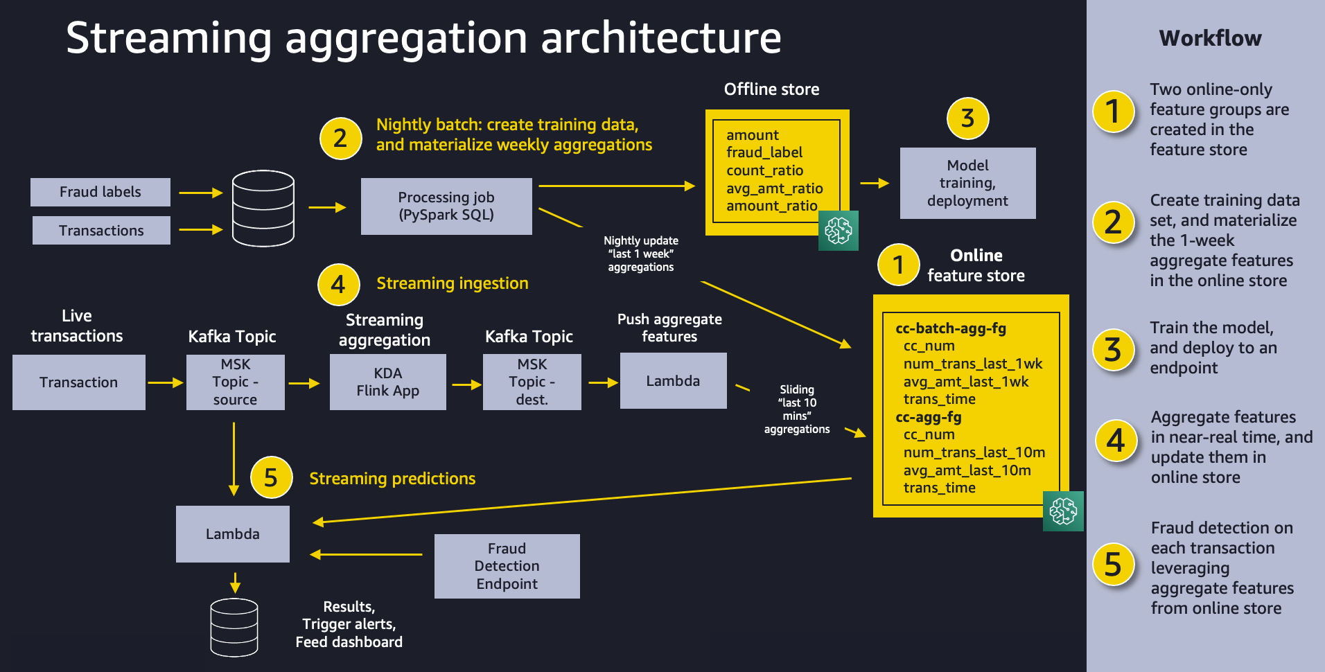
The following diagram shows our overall solution architecture. We feel that this same pattern will work well for a variety of streaming aggregation use cases. At a high level, the pattern involves the following five pieces:
We provide an AWS CloudFormation template to create the prerequisite resources for this solution. The following table lists the stacks available for different Regions.
| AWS Region | Link |
| us-east-1 | |
| us-east-2 | |
| us-west-1 | |
| eu-west-1 | |
| ap-northeast-1 |
In the following sections, we explore each component of our solution in more detail.
ML models rely on well-engineered features coming from a variety of data sources, with transformations as simple as calculations or as complicated as a multi-step pipeline that takes hours of compute time and complex coding. Feature Store enables the reuse of these features across teams and models, which improves data scientist productivity, speeds up time to market, and ensures consistency of model input.
Each feature inside Feature Store is organized into a logical grouping called a feature group. You decide which feature groups you need for your models. Each one can have dozens, hundreds, or even thousands of features. Feature groups are managed and scaled independently, but they’re all available for search and discovery across teams of data scientists responsible for many independent ML models and use cases.
ML models often require features from multiple feature groups. A key aspect of a feature group is how often its feature values need to be updated or materialized for downstream training or inference. You refresh some features hourly, nightly, or weekly, and a subset of features must be streamed to the feature store in near-real time. Streaming all feature updates would lead to unnecessary complexity, and could even lower the quality of data distributions by not giving you the chance to remove outliers.
In our use case, we create a feature group called cc-agg-batch-fg for aggregated credit card features updated in batch, and one called cc-agg-fg for streaming features.
The cc-agg-batch-fg feature group is updated nightly, and provides aggregate features looking back over a 1-week time window. Recalculating 1-week aggregations on streaming transactions don’t offer meaningful signals, and would be a waste of resources.
Conversely, our cc-agg-fg feature group must be updated in a streaming fashion, because it offers the latest transaction counts and average transaction amounts looking back over a 10-minute time window. Without streaming aggregation, we couldn’t spot the typical fraud attack pattern of a rapid sequence of purchases.
By isolating features that are recalculated nightly, we can improve ingestion throughput for our streaming features. Separation lets us optimize the ingestion for each group independently. When designing for your use cases, keep in mind that models requiring features from a large number of feature groups may want to make multiple retrievals from the feature store in parallel to avoid adding excessive latency to a real-time prediction workflow.
The feature groups for our use case are shown in the following table.
| cc-agg-fg | cc-agg-batch-fg |
| cc_num (record id) | cc_num (record id) |
| trans_time | trans_time |
| num_trans_last_10m | num_trans_last_1w |
| avg_amt_last_10m | avg_amt_last_1w |
Each feature group must have one feature used as a record identifier (for this post, the credit card number). The record identifier acts as a primary key for the feature group, enabling fast lookups as well as joins across feature groups. An event time feature is also required, which enables the feature store to track the history of feature values over time. This becomes important when looking back at the state of features at a specific point in time.
In each feature group, we track the number of transactions per unique credit card and its average transaction amount. The only difference between our two groups is the time window used for aggregation. We use a 10-minute window for streaming aggregation, and a 1-week window for batch aggregation.
With Feature Store, you have the flexibility to create feature groups that are offline only, online only, or both online and offline. An online store provides high-throughput writes and low-latency retrievals of feature values, which is ideal for online inference. An offline store is provided using Amazon Simple Storage Service (Amazon S3), giving firms a highly scalable repository, with a full history of feature values, partitioned by feature group. The offline store is ideal for training and batch scoring use cases.
When you enable a feature group to provide both online and offline stores, SageMaker automatically synchronizes feature values to an offline store, continuously appending the latest values to give you a full history of values over time. Another benefit of feature groups that are both online and offline is that they help avoid the problem of training and inference skew. SageMaker lets you feed both training and inference with the same transformed feature values, ensuring consistency to drive more accurate predictions. The focus in our post is to demonstrate online feature streaming, so we implemented online-only feature groups.
To materialize our batch features, we create a feature pipeline that runs as a SageMaker Processing job on a nightly basis. The job has two responsibilities: producing the dataset for training our model, and populating the batch feature group with the most up-to-date values for aggregate 1-week features, as shown in the following diagram.

Each historical transaction used in the training set is enriched with aggregated features for the specific credit card involved in the transaction. We look back over two separate sliding time windows: 1 week back, and the preceding 10 minutes. The actual features used to train the model include the following ratios of these aggregated values:
avg_amt_last_10m / avg_amt_last_1wtransaction_amount / avg_amt_last_1wnum_trans_last_10m / num_trans_last_1wFor example, count_ratio is the transaction count from the prior 10 minutes divided by the transaction count from the last week.
Our ML model can learn patterns of normal activity vs. fraudulent activity from these ratios, rather than relying on raw counts and transaction amounts. Spending patterns on different cards vary greatly, so normalized ratios provide a better signal to the model than the aggregated amounts themselves.
You may be wondering why our batch job is computing features with a 10-minute lookback. Isn’t that only relevant for online inference? We need the 10-minute window on historical transactions to create an accurate training dataset. This is critical for ensuring consistency with the 10-minute streaming window that will be used in near-real time to support online inference.
The resulting training dataset from the processing job can be saved directly as a CSV for model training, or it can be bulk ingested into an offline feature group that can be used for other models and by other data science teams to address a wide variety of other use cases. For example, we can create and populate a feature group called cc-transactions-fg. Our training job can then pull a specific training dataset based on the needs for our specific model, selecting specific date ranges and a subset of features of interest. This approach enables multiple teams to reuse feature groups and maintain fewer feature pipelines, leading to significant cost savings and productivity improvements over time. This example notebook demonstrates the pattern of using Feature Store as a central repository from which data scientists can extract training datasets.
In addition to creating a training dataset, we use the PutRecord API to put the 1-week feature aggregations into the online feature store nightly. The following code demonstrates putting a record into an online feature group given specific feature values, including a record identifier and an event time:
ML engineers often build a separate version of feature engineering code for online features based on the original code written by data scientists for model training. This can deliver the desired performance, but is an extra development step, and introduces more chance for training and inference skew. In our use case, we show how using SQL for aggregations can enable a data scientist to provide the same code for both batch and streaming.
Feature Store delivers single-digit millisecond retrieval of pre-calculated features, and it can also play an effective role in solutions requiring streaming ingestion. Our use case demonstrates both. Weekly lookback is handled as a pre-calculated feature group, materialized nightly as shown earlier. Now let’s dive into how we calculate features aggregated on the fly over a 10-minute window and ingest them into the feature store for later online inference.
In our use case, we ingest live credit card transactions to a source MSK topic, and use a Kinesis Data Analytics for Apache Flink application to create aggregate features in a destination MSK topic. The application is written using Apache Flink SQL. Flink SQL makes it simple to develop streaming applications using standard SQL. It’s easy to learn Flink if you have ever worked with a database or SQL-like system by remaining ANSI-SQL 2011 compliant. Apart from SQL, we can build Java and Scala applications in Amazon Kinesis Data Analytics using open-source libraries based on Apache Flink. We then use a Lambda function to read the destination MSK topic and ingest the aggregate features into a SageMaker feature group for inference. Creating the Apache Flink application using Flink’s SQL API is straightforward. We use Flink SQL to aggregate the streaming data in the source MSK topic and store it in a destination MSK topic.
To produce aggregate counts and average amounts looking back over a 10-minute window, we use the following Flink SQL query on the input topic and pipe the results to the destination topic:
| cc_num | amount | datetime | num_trans_last_10m | avg_amt_last_10m |
| …1248 | 50.00 | Nov-01,22:01:00 | 1 | 74.99 |
| …9843 | 99.50 | Nov-01,22:02:30 | 1 | 99.50 |
| …7403 | 100.00 | Nov-01,22:03:48 | 1 | 100.00 |
| …1248 | 200.00 | Nov-01,22:03:59 | 2 | 125.00 |
| …0732 | 26.99 | Nov01, 22:04:15 | 1 | 26.99 |
| …1248 | 50.00 | Nov-01,22:04:28 | 3 | 100.00 |
| …1248 | 500.00 | Nov-01,22:05:05 | 4 | 200.00 |
In this example, notice that the final row has a count of four transactions in the last 10 minutes from the credit card ending with 1248, and a corresponding average transaction amount of $200.00. The SQL query is consistent with the one used to drive creation of our training dataset, helping to avoid training and inference skew.
As transactions stream into the Kinesis Data Analytics for Apache Flink aggregation app, the app sends the aggregate results to our Lambda function, as shown in the following diagram. The Lambda function takes these features and populates the cc-agg-fg feature group.

We send the latest feature values to the feature store from Lambda using a simple call to the PutRecord API. The following is the core piece of Python code for storing the aggregate features:
We prepare the record as a list of named value pairs, including the current time as the event time. The Feature Store API ensures that this new record follows the schema that we identified when we created the feature group. If a record for this primary key already existed, it is now overwritten in the online store.
Now that we have streaming ingestion keeping the feature store up to date with the latest feature values, let’s look at how we make fraud predictions.
We create a second Lambda function that uses the source MSK topic as a trigger. For each new transaction event, the Lambda function first retrieves the batch and streaming features from Feature Store. To detect anomalies in credit card behavior, our model looks for spikes in recent purchase amounts or purchase frequency. The Lambda function computes simple ratios between the 1-week aggregations and the 10-minute aggregations. It then invokes the SageMaker model endpoint using those ratios to make the fraud prediction, as shown in the following diagram.

We use the following code to retrieve feature values on demand from the feature store before calling the SageMaker model endpoint:
SageMaker also supports retrieving multiple feature records with a single call, even if they are from different feature groups.
Finally, with the model input feature vector assembled, we call the model endpoint to predict if a specific credit card transaction is fraudulent. SageMaker also supports retrieving multiple feature records with a single call, even if they are from different feature groups.
sagemaker_runtime =
    boto3.client(service_name='runtime.sagemaker')
request_body = ','.join(features)
response = sagemaker_runtime.invoke_endpoint(
    EndpointName=ENDPOINT_NAME,
    ContentType='text/csv',
    Body=request_body)
probability = json.loads(response['Body'].read().decode('utf-8'))
In this example, the model came back with a probability of 98% that the specific transaction was fraudulent, and it was able to use near-real-time aggregated input features based on the most recent 10 minutes of transactions on that credit card.
To demonstrate the full end-to-end workflow of our solution, we simply send credit card transactions into our MSK source topic. Our automated Kinesis Data Analytics for Apache Flink aggregation takes over from there, maintaining a near-real-time view of transaction counts and amounts in Feature Store, with a sliding 10-minute lookback window. These features are combined with the 1-week aggregate features that were already ingested to the feature store in batch, letting us make fraud predictions on each transaction.
We send a single transaction from three different credit cards. We then simulate a fraud attack on a fourth credit card by sending many back-to-back transactions in seconds. The output from our Lambda function is shown in the following screenshot. As expected, the first three one-off transactions are predicted as NOT FRAUD. Of the 10 fraudulent transactions, the first is predicted as NOT FRAUD, and the rest are all correctly identified as FRAUD. Notice how the aggregate features are kept current, helping drive more accurate predictions.

We have shown how Feature Store can play a key role in the solution architecture for critical operational workflows that need streaming aggregation and low-latency inference. With an enterprise-ready feature store in place, you can use both batch ingestion and streaming ingestion to feed feature groups, and access feature values on demand to perform online predictions for significant business value. ML features can now be shared at scale across many teams of data scientists and thousands of ML models, improving data consistency, model accuracy, and data scientist productivity. Feature Store is available now, and you can try out this entire example. Let us know what you think.
Special thanks to everyone who contributed to the previous blog post with a similar architecture: Paul Hargis, James Leoni and Arunprasath Shankar.
 Mark Roy is a Principal Machine Learning Architect for AWS, helping customers design and build AI/ML solutions. Mark’s work covers a wide range of ML use cases, with a primary interest in feature stores, computer vision, deep learning, and scaling ML across the enterprise. He has helped companies in many industries, including insurance, financial services, media and entertainment, healthcare, utilities, and manufacturing. Mark holds six AWS certifications, including the ML Specialty Certification. Prior to joining AWS, Mark was an architect, developer, and technology leader for over 25 years, including 19 years in financial services.
 Raj Ramasubbu is a Senior Analytics Specialist Solutions Architect focused on big data and analytics and AI/ML with Amazon Web Services. He helps customers architect and build highly scalable, performant, and secure cloud-based solutions on AWS. Raj provided technical expertise and leadership in building data engineering, big data analytics, business intelligence, and data science solutions for over 18 years prior to joining AWS. He helped customers in various industry verticals like healthcare, medical devices, life science, retail, asset management, car insurance, residential REIT, agriculture, title insurance, supply chain, document management, and real estate.
 Prabhakar Chandrasekaran is a Senior Technical Account Manager with AWS Enterprise Support. Prabhakar enjoys helping customers build cutting-edge AI/ML solutions on the cloud. He also works with enterprise customers providing proactive guidance and operational assistance, helping them improve the value of their solutions when using AWS. Prabhakar holds six AWS and six other professional certifications. With over 20 years of professional experience, Prabhakar was a data engineer and a program leader in the financial services space prior to joining AWS.

This is a guest post co-written with Fred Wu from Sportradar.
Sportradar is the world’s leading sports technology company, at the intersection between sports, media, and betting. More than 1,700 sports federations, media outlets, betting operators, and consumer platforms across 120 countries rely on Sportradar knowhow and technology to boost their business.
Sportradar uses data and technology to:
This post demonstrates how Sportradar used Amazon’s Deep Java Library (DJL) on AWS alongside Amazon Elastic Kubernetes Service (Amazon EKS) and Amazon Simple Storage Service (Amazon S3) to build a production-ready machine learning (ML) inference solution that preserves essential tooling in Java, optimizes operational efficiency, and increases the team’s productivity by providing better performance and accessibility to logs and system metrics.
The DJL is a deep learning framework built from the ground up to support users of Java and JVM languages like Scala, Kotlin, and Clojure. Right now, most deep learning frameworks are built for Python, but this neglects the large number of Java developers and developers who have existing Java code bases they want to integrate the increasingly powerful capabilities of deep learning into. With the DJL, integrating this deep learning is simple.
In this post, the Sportradar team discusses the challenges they encountered and the solutions they created to build their model inference platform using the DJL.
We are the US squad of the Sportradar AI department. Since 2018, our team has been developing a variety of ML models to enable betting products for NFL and NCAA football. We recently developed four more new models.
The fourth down decision models for the NFL and NCAA predict the probabilities of the outcome of a fourth down play. A play outcome could be a field goal attempt, play, or punt.
The drive outcome models for the NFL and NCAA predict the probabilities of the outcome of the current drive. A drive outcome could be an end of half, field goal attempt, touchdown, turnover, turnover on downs, or punt.

Our models are the building blocks of other models where we generate a list of live betting markets, include spread, total, win probability, next score type, next team to score, and more.
The business requirements for our models are as follows:
The main challenge we have is how to bridge the gap between model training in Python and model inference in Java. Our data scientists train the model in Python using tools like PyTorch and save the model as PyTorch scripts. Our original plan was to also host the models in Python and utilize gRPC to communicate with another service, which will use the Java gRPC client to send the request.
However, a few issues came with this solution. Mainly, we saw the network overhead between two different services running in separate run environments or pods, which resulted in higher latency. But the maintenance overhead was the main reason we abandoned this solution. We had to build both the gRPC server and the client program separately and keep the protocol buffer files consistent and up to date. Then we needed to Dockerize the application, write a deployment YAML file, deploy the gRPC server to our Kubernetes cluster, and make sure it’s reliable and auto scalable.
Another problem was whenever an error occurred on the gRPC server side, the application client only got a vague error message instead of a detailed error traceback. The client had to reach out to the gRPC server maintainer to learn exactly which part of the code caused the error.
Ideally, we instead want to load the model PyTorch scripts, extract the features from model input, and run model inference entirely in Java. Then we can build and publish it as a Maven library, hosted on our internal registry, which our service team could import into their own Java projects. When we did our research online, the Deep Java Library showed up on the top. After reading a few blog posts and DJL’s official documentation, we were sure DJL would provide the best solution to our problem.
The following diagram compares the previous and updated architecture.

The following diagram outlines the workflow of the DJL solution.

The steps are as follows:
We have seen a stable inferencing runtime and reliable prediction results. The DJL solution offers several advantages over gRPC-based solutions:
The DJL is a full deep learning framework that supports the deep learning lifecycle from building a model, training it on a dataset, to deploying it in production. It has intuitive helpers and utilities for modalities like computer vision, natural language processing, audio, time series, and tabular data. DJL also features an easy model zoo of hundreds of pre-trained models that can be used out of the box and integrated into existing systems.
It is also a fully Apache-2 licensed open-source project and can be found on GitHub. The DJL was created at Amazon and open-sourced in 2019. Today, DJL’s open-source community is led by Amazon and has grown to include many countries, companies, and educational institutions. The DJL continues to grow in its ability to support different hardware, models, and engines. It also includes support for new hardware like ARM (both in servers like AWS Graviton and laptops with Apple M1) and AWS Inferentia.
The architecture of DJL is engine agnostic. It aims to be an interface describing what deep learning could look like in the Java language, but leaves room for multiple different implementations that could provide different capabilities or hardware support. Most popular frameworks today such as PyTorch and TensorFlow are built using a Python front end that connects to a high-performance C++ native backend. The DJL can use this to connect to these same native backends to take advantage of their work on hardware support and performance.
For this reason, many DJL users also use it for inference only. That is, they will train a model using Python and then load it using the DJL for deployment as part of their existing Java production system. Because the DJL utilizes the same engine that powers Python, it’s able to run without any decrease in performance or loss in accuracy. This is exactly the strategy that we found to support the new models.
The following diagram illustrates the workflow under the hood.

When the DJL loads, it finds all the engine implementations available in the class path using Java’s ServiceLoader. In this case, it detects the DJL PyTorch engine implementation, which will act as the bridge between the DJL API and the PyTorch Native.
The engine then works to load the PyTorch Native. By default, it downloads the appropriate native binary based on your OS, CPU architecture, and CUDA version, making it almost effortless to use. You can also provide the binary using one of the many available native JAR files, which are more reliable for production environments that often have limited network access for security.
Once loaded, the DJL uses the Java Native Interface to translate all the easy high-level functionalities in DJL into the equivalent low-level native calls. Every operation in the DJL API is hand-crafted to best fit the Java conventions and make it easily accessible. This also includes dealing with native memory, which is not supported by the Java Garbage Collector.
Although all these details are within the library, calling it from a user standpoint couldn’t be easier. In the following section, we walk through this process.
Because we train our models using PyTorch, we use the DJL’s PyTorch engine for the model inference.
Loading the model is incredibly easy. All it takes is to build a criteria describing the model to load and where it is from. Then, we load it and use the model to create a new predictor session. See the following code:

For our model, we also have a custom translator, which we call MyTranslator. We use the translator to encapsulate the preprocessing code that converts from a convenient Java type into the input expected by the model and the postprocessing code that converts from the model output into a convenient output. In our case, we chose to use a float[] as the input type and the built-in DJL classifications as the output type. The following is a snippet of our translator code:

It’s pretty amazing that with just a few lines of code, the DJL loads the PyTorch scripts and our custom translator, and then the predictor is ready to make the predictions.
Sportradar’s product built on the DJL solution went live before the 2022–23 NFL regular season started, and it has been running smoothly since then. In the future, Sportradar plans to re-platform existing models hosted on gRPC servers to the DJL solution.
The DJL continues to grow in many different ways. The most recent release, v0.21.0, has many improvements, including updated engine support, improvements on Spark, Hugging Face batch tokenizers, an NDScope for easier memory management, and enhancements to the time series API. It also has the first major release of DJL Zero, a new API aiming to allow support for both using pre-trained models and training your own custom deep learning models even with zero knowledge of deep learning.
The DJL also features a model server called DJL Serving. It makes it simple to host a model on an HTTP server from any of the 10 supported engines, including the Python engine to support Python code. With v0.21.0 of DJL Serving, it includes faster transformer support, Amazon SageMaker multi-model endpoint support, updates for Stable Diffusion, improvements for DeepSpeed, and updates to the management console. You can now use it to deploy large models with model parallel inference using DeepSpeed and SageMaker.
There is also much upcoming with the DJL. The largest area under development is large language model support for models like ChatGPT or Stable Diffusion. There is also work to support streaming inference requests in DJL Serving. Thirdly, there are improvements to demos and the extension for Spark. Of course, there is also standard continuing work including features, fixes, engine updates, and more.
For more information on the DJL and its other features, see Deep Java Library.
Follow our GitHub repo, demo repository, Slack channel, and Twitter for more documentation and examples of the DJL!
 Fred Wu is a Senior Data Engineer at Sportradar, where he leads infrastructure, DevOps, and data engineering efforts for various NBA and NFL products. With extensive experience in the field, Fred is dedicated to building robust and efficient data pipelines and systems to support cutting-edge sports analytics.
 Zach Kimberg is a Software Developer in the Amazon AI org. He works to enable the development, training, and production inference of deep learning. There, he helped found and continues to develop the DeepJavaLibrary project.
 Kanwaljit Khurmi is a Principal Solutions Architect at Amazon Web Services. He works with the AWS customers to provide guidance and technical assistance helping them improve the value of their solutions when using AWS. Kanwaljit specializes in helping customers with containerized and machine learning applications.

Shanghai is once again showing why it’s called the “Magic City” as more than 1,000 exhibitors from 20 countries dazzle the automotive world this week at the highly anticipated International Automobile Industry Exhibition.
With nearly 1,500 vehicles on display, the 20th edition of Auto Shanghai is showcasing the newest AI-powered cars and mobility solutions using the NVIDIA DRIVE Hyperion compute platform built on the DRIVE Orin system-on-chip (SoC).
SAIC Motor’s Rising Auto brand unveiled the recently launched mid-to-large luxury pure electric sedan F7 and mid-to-large luxury pure electric SUV R7 at the show, both of which feature an advanced intelligent-driving system built on NVIDIA DRIVE Orin. Equipped with a swappable battery pack, the F7 is built to go the distance with up to a 413-mile range.

New energy vehicle (NEV) maker GAC AION showcased its flagship model Hyper GT, which is available for pre-sale. Equipped with the high-performance NVIDIA DRIVE Orin SoC, the car is designed to support advanced level 2+ driving capabilities in high-speed environments. Featuring an array of aerodynamic features that minimize drag, the Hyper GT has a wind resistance coefficient of just 0.19 Cd, the lowest of any production car in the world, GAC Aion claims.

At the show, EV maker XPENG showcased its full range of models including the all-new P7i ultra-smart coupe and XPENG G9, a super-fast-charging, intelligent SUV, built on the high-performance DRIVE Orin centralized compute architecture to deliver AI capabilities that are continuously upgradable through over-the-air updates.
XPENG also debuted the first model under its SEPA 2.0 Soaring architecture — the XPENG G6 — also powered by NVIDIA DRIVE Orin. As an intelligent driving coupe SUV, the XPENG G6 is based on a high-voltage 800V silicon carbide platform that XPENG launched globally, and is also equipped with its proprietary XNGP intelligent assisted driving system.

Elsewhere on the show floor, IM Motors, a joint venture among China’s SAIC Motor, Alibaba and Shanghai’s Zhangjiang Group, exhibited its flagship LS7 SUV and the L7 sedan powered by NVIDIA DRIVE Orin. IM Motors reports that it has launched its capability for highway navigation on autopilot — users will be able to experience it on the L7 and LS7 soon.
NEV maker Human Horizons officially took the wraps off its HiPhi Y SUV, the latest addition to its lineup of intelligent vehicles. The vehicle’s marquee features include a wing-door design, a China light-duty vehicle test cycle (CLTC) range of more than 497 miles on a single charge, and an autonomous-driving system powered by DRIVE Orin.
This is the second model stemming from HiPhi’s cooperation with NVIDIA. The NEV company last summer launched HiPhi Z, the digital grand tourer equipped with the HiPhi Pilot intelligent driver-assistance system. The system features NVIDIA DRIVE Orin and a 30+ sensor suite to support functions such as assisted driving.
As China NEV makers look to expand their global footprint, HiPhi also announced it will bring its vehicles to select countries in Western Europe and Scandinavia. This includes HiPhi X, HiPhi Z and HiPhi Y.

Premium smart electric vehicle company NIO revealed the ES6 SUV during Auto Shanghai. NIO’s family of smart vehicles are being showcased at the NIO booth, including an updated version of its ET7, along with the ES8, EC7, ES7, ES6 and ET5. All these vehicles run on its proprietary Adam supercomputer, which is powered by four NVIDIA DRIVE Orin SoCs. This quad configuration delivers 1,016 TOPS of performance to enable advanced driver-assistance systems and a point-to-point autonomous driving experience.
NIO also recently announced it’s equipping its third-generation powerswap station with two laser radars and two NVIDIA DRIVE Orin SoCs, with a total computing power of 508 TOPS, which enables the Automatic Summon and Swap feature, which enables the station to communicate with the vehicle and automatically navigate the vehicle for a battery swap.

Li Auto displayed three of its flagship models, including the L9, L8 Max and L7 Max. These models feature dual NVIDIA DRIVE Orin SoCs to power its intelligent-driving system, the Ideal AD Max, delivering 508 TOPS of computing power to help the vehicle efficiently process data from high-definition cameras, lidars, millimeter-wave radars and ultrasonic sensors in real time.
Li Auto also released an 800V supercharged pure electric solution, which can travel 248 miles after charging for 10 minutes. The automaker demonstrated AD Max 3.0, which is also powered by NVIDIA DRIVE Orin. The company’s urban NOA navigation assisted-driving system will be released in the second quarter of this year. And by the end of the year, this all-scenario navigation-assisted driving system will cover 100 cities in China.
Swedish premium automaker Volvo Cars debuted its all-electric EX90 in China. Revealed in November last year, the state-of-the-art, software-defined SUV features a new powertrain and cutting-edge technology to deliver the ultimate in safety and intelligence with the AI compute of NVIDIA DRIVE Orin and Xavier platforms.
During its Volvo Cars Tech Day held earlier this week, the automaker also unveiled its EX90 Excellence, the top-of-the-line and limited edition of the EX90. The four-seater SUV features a two-tone exterior, outstanding comfort inside and an intelligent technology base powered by NVIDIA DRIVE.

Lotus brought its three champion products to the Auto Shanghai, including the first electric Hyper-SUV Lotus Eletre, the first pure electric hypercar Evija and Emira, the last internal combustion engine sports car from Lotus. The Lotus Eletre is equipped with the cockpit-forward design inspired by Evija and embodies the essence of aesthetics. It features an immersive digital cockpit, long battery range of the Eletre S+ version up to 403 miles and autonomous-driving capabilities powered by the NVIDIA DRIVE Orin.
Tier-1 suppliers for the auto industry and emerging self-driving companies also presented their latest offerings at Auto Shanghai.
Desay SV is pushing the boundaries of autonomous-driving performance with its latest solutions for smart cockpit, intelligent driving and connected services. The mobility company demonstrated its DRIVE Orin-based smart cockpit solution, which is part of the ICPAurora Intelligent Centralized Computing Platform, for powering new forms of in-vehicle infotainment, including 3D gaming and Android-based systems.
Desay SV’s integration of cabin and autonomous driving showcases centralizing all intelligent vehicle functions on a single NVIDIA DRIVE computer. Announced last September, the NVIDIA DRIVE Thor SoC is the successor to DRIVE Orin, delivering 2,000 teraflops of performance and designed to centralized automated driving and AI cockpit functions on a single platform. DRIVE Thor is targeting automakers’ 2025 models.
Baidu Apollo showcased its level-2 driver-assisted product Apollo City Driving Max intelligent driving computing unit, featuring a Baidu-developed intelligent-driving domain controller and powered by two NVIDIA DRIVE Orin SoCs to process camera and lidar sensor data for enhanced safety behind the wheel. The company reports the Apollo City Driving Max will be available in volume production to automakers globally in 2023.
Momenta launched Mpilot Pro, its new advanced driver-assistance solution. The solution adopts the energy-efficient DRIVE Orin to meet the computing performance requirements of mainstream mid-range models. In addition, DRIVE Orin’s compatible architecture scales from level 2+ ADAS to level 5 autonomous driving.
The NVIDIA DRIVE ecosystem can be found throughout this year’s Auto Shanghai — showcasing how NVIDIA is leading the charge toward a future of intelligent vehicles that deliver higher levels of safety, convenience and enjoyment on the road.

 Posted by Thushan Ganegedara (GDE), Haidong Rong (Nvidia), Wei Wei (Google)

Modern recommenders heavily leverage embeddings to create vector representations of each user and candidate item. These embedding can then be used to calculate the similarity between users and items, so that users are recommended candidate items that are more interesting and relevant. But when working with data at scale, particularly in an online machine learning setting, embedding tables can grow in size dramatically, accumulating millions (and sometimes billions) of items. At this scale, it becomes impossible to store these embedding tables in memory. Furthermore, a large portion of the items might be rarely seen, so it does not make sense to keep dedicated embeddings for such rarely occurring items. A better solution would be to represent those items with one common embedding. This can dramatically reduce the size of the embedding table at a very small fraction of the performance cost. This is the main motivation behind dynamic embedding tables.
TensorFlow’s built-in tf.keras.layers.Embedding layer has a fixed size at creation time, so we need another approach. Fortunately, there is a TensorFlow SIG project exactly for this purpose: TensorFlow Recommenders Addons (TFRA). You can learn more from its repository, but at a high level TFRA leverages dynamic embedding technology to dynamically change embedding size and achieve better recommendation results than static embeddings. TFRA is fully TF2.0-compatible and works smoothly with the familiar Keras API interfaces, so it can be easily integrated with other TensorFlow products, such as TensorFlow Recommenders (TFRS).
In this tutorial we will build a movie recommender model by leveraging both TFRS and TFRA. We will use the MovieLens dataset, which contains anonymized data showing ratings given to movies by users. Our primary focus is to show how the dynamic embeddings provided in the TensorFlow Recommenders Addons library can be used to dynamically grow and shrink the size of the embedding tables in the recommendation setting. You can find the full implementation here and a walkthrough here.
Let’s first build a baseline model with TensorFlow Recommenders. We will follow the pattern of this TFRS retrieval tutorial to build a two-tower retrieval model. The user tower will take the user ID as the input, but the item tower will use the tokenized movie title as the input.
To handle the movie titles, we define a helper function that converts the movie titles to lowercase, removes any punctuation in a given movie title, and splits using spaces to generate a list of tokens. Finally we take only the up to max_token_length tokens (from the start) from the movie title. If a movie title has fewer tokens, all the tokens will be taken. This number is chosen based on some analysis and represents the 90th percentile in the title lengths in the dataset.
max_token_length = 6 |
We also pad the tokenized movie titles to a fixed length and split the dataset using the same random seed so that we get consistent validation results across training epochs. You can find detailed code in the ‘Processing datasets’ section of the notebook.
Our user tower is pretty much the same as in the TFRS retrieval tutorial (except it’s deeper), but for the movie tower there is a GlobalAveragePooling1D layer after the embedding lookup, which averages the embedding of movie title tokens to a single embedding.
def get_movie_title_lookup_layer(dataset: tf.data.Dataset) -> tf.keras.layers.Layer: |
Next we are going to train the model.
Training the model is simply calling fit() on the model with the required arguments. We will be using our validation dataset validation_ds to measure the performance of our model.
history = model.fit(datasets.training_datasets.train_ds, epochs=3, validation_data=datasets.training_datasets.validation_ds) |
At the end, the output looks like below:
Epoch 3/3 |
We have achieved a top 100 categorical accuracy of 13.38% on the validation dataset.
We will now learn how we can use the dynamic embedding in the TensorFlow Recommenders Addons (TFRA) library, rather than a static embedding table. As the name suggests, as opposed to creating embeddings for all the items in the vocabulary up front, dynamic embedding would only grow the size of the embedding table on demand. This behavior really shines when dealing with millions and billions of items and users as some companies do. For these companies, it’s not surprising to find static embedding tables that would not fit in memory. Static embedding tables can grow up to hundreds of Gigabytes or even Terabytes, incapacitating even the highest memory instances available in cloud environments.
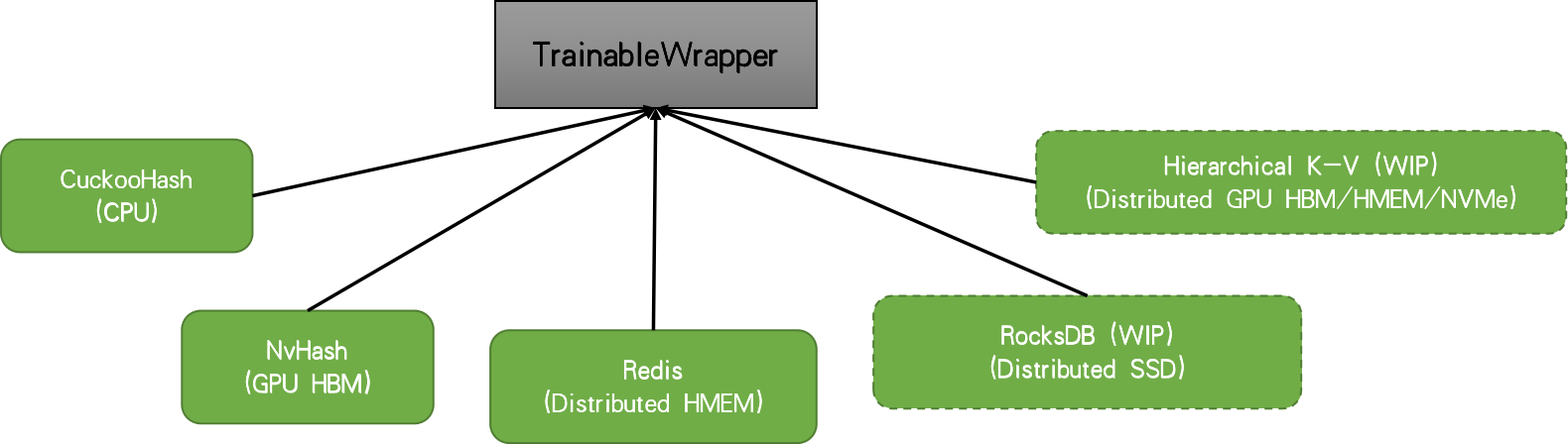
When you have an embedding table with large cardinality, the accessing weights will be quite sparse. Therefore, a hash-table based data structure is used to hold the weights and required weights for each iteration are retrieved from the underlying table structure. Here, to focus on the core functionality of the library, we will focus on a non-distributed setting. In this case, TFRA will choose cuckoo hashtable by default. But there are other solutions such as Redis, nvhash available.
 |
When using the dynamic embedding, we initialize the table with some initial capacity and the table will grow in size on demand as it sees more IDs during model training. For more information about motivation and inner mechanics, please refer to the RFC.
Currently in the TFRA dynamic_embedding module, there are three types of embedding available:
n_slots as an argument and IDs are mapped to a slot within the layer. The layer would return a tensor of size [batch_size, n_slots, embedding_dim]. We will be using the Embedding to represent the user IDs and SquashedEmbedding to represent token IDs. Remember that each movie title has multiple tokens, therefore, we need a way to reduce the resulting token embeddings to a single representative embedding.
Note: The behavior of Embedding has changed from version 0.5 to 0.6. Please make sure to use version 0.6 for this tutorial.
With that, we can define the two towers as we did in the standard model. However, this time we’ll be using the dynamic embedding layers instead of static embedding layers.
def build_de_user_model(user_id_lookup_layer: tf.keras.layers.StringLookup) -> tf.keras.layers.Layer: |
With the user tower and movie tower models defined, we can define the retrieval model as usual.
As a final step in model building, we’ll create the model and compile it.
def create_de_two_tower_model(dataset: tf.data.Dataset, candidate_dataset: tf.data.Dataset) -> tf.keras.Model:
|
Note the usage of the DynamicEmbeddingOptimizer wrapper around the standard TensorFlow optimizer. It is mandatory to wrap the standard optimizer in a DynamicEmbeddingOpitmizer as it will provide specialized functionality needed to train the weights stored in a hashtable. We can now train our model.
Training the model is quite straightforward, but will involve a bit more extra effort as we’d like to log some extra information. We will perform the logging through a tf.keras.callbacks.Callback object. We’ll name this DynamicEmbeddingCallback.
epochs = 3 |
We have taken the loop that goes through the epochs out of the fit() function. Then in every epoch we re-create the dataset, as that will provide a different shuffling of the training dataset. We will train the model for a single epoch within the loop. Finally we accumulate the logged embedding sizes in history_de_size (this is provided by our custom callback) and performance metrics in history_de.
The callback is implemented as follows.
class DynamicEmbeddingCallback(tf.keras.callbacks.Callback):
|
The callback does two things:
steps_per_logging iterationsrestrict=True(This is set to False by default)Let’s understand what reducing the size means and why it is important.
An important topic we still haven’t discussed is how to reduce the size of the embedding table, should it grow over some predefined threshold. This is a powerful functionality as it allows us to define a threshold over which the embedding table should not grow. This will allow us to work with large vocabularies while keeping the memory requirement under the memory limitations we may have. We achieve this by calling restrict() on the underlying variables of the embedding layer as shown in the DynamicEmbeddingCallback. restrict() takes two arguments in: num_reserved (the size after the reduction) and trigger (size at which the reduction should be triggered). The policy that governs how the reduction is performed is defined using the restrict_policy argument in the layer construct. You can see that we are using the FrequencyRestrictPolicy. This means the least frequent items will be removed from the embedding table. The callback enables a user to set how frequently the reduction should get triggered by setting the steps_per_restrict and restrict arguments in the DynamicEmbeddingCallback.
Reducing the size of the embedding table makes more sense when you have streaming data. Think about an online learning setting, where you are training the model every day (or even every hour) on some incoming data. You can think of the outer for loop (i.e. epochs) representing days. Each day you receive a dataset (containing user interactions from the previous day for example) and you train the model from the previous checkpoint. In this case, you can use the DynamicEmbeddingCallback to trigger a restrict if the embedding table grows over the size defined in the trigger argument.
Here we analyze the performance of three variants.
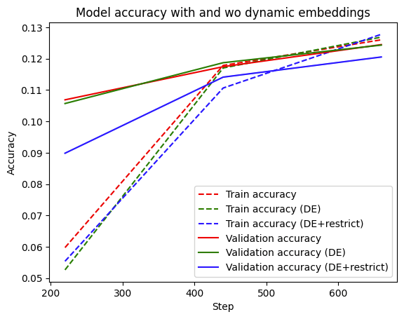 |
You can see that the model using dynamic embeddings (solid green line) has comparative validation performance to the baseline (solid red line). You can see a similar trend in the training accuracy as well. In practice, dynamic embeddings can often be seen to improve accuracy in a large-scale online learning setup.
Finally, we can see that restrict has a somewhat detrimental effect on the validation accuracy, which is understandable. Since we’re working with a relatively small dataset with a small number of items, the reduction could be getting rid of embeddings that are best kept in the table. For example, you can increase the num_reserved argument (e.g. set it to int(self.model.lookup_vocab_sizes[k]*0.95)) in the restrict function which would yield performance that improves towards the performance of without restrict.
Next we look at how dynamic the embedding tables really are over time.
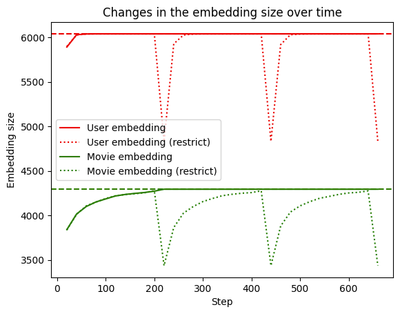 |
We can see that when restrict is not used, the embedding table grows to the full size of the vocabulary (dashed line) and stays there. However when restrict is triggered (dotted line), the size drops and grows in size again as it encounters new IDs.
It is also important to note that constructing a proper validation is not a trivial task. There are considerations such as out-of-sample validation, out-of-time validation, stratification, etc. that needs to be taken into account carefully. However for this exercise, we have not focused on such factors and created a validation set by sampling randomly from the existing dataset.
Using dynamic embedding tables is a powerful way to perform representation learning when working with large sets of items containing millions or billions of entities. In this tutorial, we learnt how to use the dynamic_embedding module provided in the TensorFlow Recommender Addons library to achieve this. We first explored the data and constructed tf.data.Dataset objects by extracting the features we’ll be using for our model training and evaluation. Next we defined a model that uses static embedding tables to use as an evaluation baseline. We then created a model that uses dynamic embedding and trained it on the data. We saw that using dynamic embeddings, the embedding tables grow only on demand and still achieve comparable performance with the baseline. We also discussed how the restrict functionality can be used to shrink the embedding table if it grows past a pre-defined threshold.
We hope this tutorial gives you a good conceptual introduction to TFRA and dynamic embeddings, and helps you think about how you can leverage it to enhance your own recommenders. If you would like to have a more in-depth discussion, please visit the TFRA repository.