Drawing from philosophy to identify fair principles for ethical AI…Read More

Drawing from philosophy to identify fair principles for ethical AI…Read More
Drawing from philosophy to identify fair principles for ethical AI…Read More

As artificial intelligence (AI) becomes more powerful and more deeply integrated into our lives, the questions of how it is used and deployed are all the more important. What values guide AI? Whose values are they? And how are they selected?Read More

From climate modeling to endangered species conservation, developers, researchers and companies are keeping an AI on the environment with the help of NVIDIA technology.
They’re using NVIDIA GPUs and software to track endangered African black rhinos, forecast the availability of solar energy in the U.K., build detailed climate models and monitor environmental disasters from satellite imagery.
This Earth Day, discover five key ways AI and accelerated computing are advancing sustainability, climate science and energy efficiency.
To protect endangered species, camera-enabled edge AI devices embedded in the environment or on drones can help scientists observe animals in the wild, monitoring their populations and detecting threats from predators and poachers.
Conservation AI, a U.K.-based nonprofit, has deployed 70+ cameras around the world powered by NVIDIA Jetson modules for edge AI. Together with the NVIDIA Triton Inference Server, the Conservation AI platform can identify species of interest from footage in just four seconds — and help conservationists detect poachers and rapidly intervene. Another research team developed an NVIDIA Jetson-based solution to monitor endangered black rhinos in Namibia using drone-based AI.

And artist Sofia Crespo raised awareness for critically endangered plants and animals through a generative AI art display at Times Square, using generative adversarial networks trained on NVIDIA GPUs to create high-resolution visuals representing relatively unknown species.
In the field of agriculture, Bay Area startup Verdant and smart tractor company Monarch Tractor are developing AI to support sustainable farming practices, including precision spraying to reduce the use of herbicides.
NVIDIA AI and high performance computing are advancing nearly every field of renewable energy research.
Open Climate Fix, a nonprofit product lab and member of the NVIDIA Inception program for startups, is developing AI models that can help predict cloud cover over solar panels — helping electric grid operators determine how much solar energy can be generated that day to help meet customers’ power needs. Startups Utilidata and Anuranet are developing AI-enabled electric meters using NVIDIA Jetson to enable a more energy efficient, resilient grid.
Siemens Gamesa Renewable Energy is working with NVIDIA to create physics-informed digital twins of wind farms using NVIDIA Omniverse and NVIDIA Modulus. U.K. company Zenotech used cloud-based GPUs to accurately simulate the likely energy output of a wind farm’s 140 turbines. And Gigastack, a consortium-led project, is using Omniverse to build a proof of concept for a wind farm that will turn water into hydrogen fuel.
Researchers at Lawrence Livermore National Laboratory achieved a breakthrough in fusion energy using HPC simulations running on Sierra, the world’s sixth-fastest HPC system, which has 17,280 NVIDIA GPUs. And the U.K.’s Atomic Energy Authority is testing the NVIDIA Omniverse simulation platform to design a fusion energy power plant.
Accurately modeling the atmosphere is critical to predicting climate change in the coming decades.
To better predict extreme weather events, NVIDIA created FourCastNet, a physics-ML model that can forecast the precise path of catastrophic atmospheric rivers a full week in advance.
Using Omniverse, NVIDIA and Lockheed Martin are building an AI-powered digital twin for the U.S. National Oceanic and Atmospheric Administration that could significantly reduce the amount of time necessary to generate complex weather visualizations.
An initiative from Northwestern University and Argonne National Laboratory researchers is instead taking a hyper-local approach, using NVIDIA Jetson-powered devices to better understand wildfires, urban heat islands and the effect of climate on crops.
When it’s difficult to gauge a situation from the ground, satellite data provides a powerful vantage point to monitor and manage climate disasters.
NVIDIA is working with the United Nations Satellite Centre to apply AI to the organization’s satellite imagery technology infrastructure, an initiative that will provide humanitarian teams with near-real-time insights about floods, wildfires and other climate-related disasters.
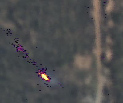
NVIDIA Inception member Masterful AI has developed machine learning tools that can detect climate risks from satellite and drone feeds. The model has been used to identify rusted transformers that could spark a wildfire and improve damage assessments after hurricanes.
San Francisco-based Inception startup Orbital Sidekick operates satellites that collect hyperspectral intelligence — information from across the electromagnetic spectrum. Its NVIDIA Jetson-powered AI solution can detect hydrocarbon or gas leaks from this data, helping reduce the risk of leaks becoming serious crises.
On its own, adopting NVIDIA tech is already a green choice: If every CPU-only server running AI and HPC worldwide switched to a GPU-accelerated system, the world could save around 20 trillion watt-hours of energy a year, equivalent to the electricity requirements of nearly 2 million U.S. homes.

Semiconductor leaders are integrating the NVIDIA cuLitho software library to accelerate the time to market and boost the energy efficiency of computational lithography, the process of designing and manufacturing next-generation chips. And the NVIDIA Grace CPU Superchip — which scored 2x performance gains over comparable x86 processors in tests — can help data centers slash their power bills by up to half.
In the most recent MLPerf inference benchmark for AI performance, the NVIDIA Jetson AGX Orin system-on-module achieved gains of up to 63% in energy efficiency, supplying AI inference at low power levels, including on battery-powered systems.
NVIDIA last year introduced a liquid-cooled NVIDIA A100 Tensor Core GPU, which Equinix evaluated for use in its data centers. Both companies found that a data center using liquid cooling could run the same workloads as an air-cooled facility while using around 30% less energy.
Startup EverestLabs developed RecycleOS, an AI software and robotics solution that helps recycling facilities around the world recover an average of 25-40% more waste, ensuring fewer recyclable materials end up in landfills. The company’s founder and CEO talked about its tech on the NVIDIA AI Podcast:
Learn more about green computing, and about NVIDIA-accelerated applications in climate and energy.

Recent deep learning advances have enabled a plethora of high-performance, real-time multimedia applications based on machine learning (ML), such as human body segmentation for video and teleconferencing, depth estimation for 3D reconstruction, hand and body tracking for interaction, and audio processing for remote communication.
However, developing and iterating on these ML-based multimedia prototypes can be challenging and costly. It usually involves a cross-functional team of ML practitioners who fine-tune the models, evaluate robustness, characterize strengths and weaknesses, inspect performance in the end-use context, and develop the applications. Moreover, models are frequently updated and require repeated integration efforts before evaluation can occur, which makes the workflow ill-suited to design and experiment.
In “Rapsai: Accelerating Machine Learning Prototyping of Multimedia Applications through Visual Programming”, presented at CHI 2023, we describe a visual programming platform for rapid and iterative development of end-to-end ML-based multimedia applications. Visual Blocks for ML, formerly called Rapsai, provides a no-code graph building experience through its node-graph editor. Users can create and connect different components (nodes) to rapidly build an ML pipeline, and see the results in real-time without writing any code. We demonstrate how this platform enables a better model evaluation experience through interactive characterization and visualization of ML model performance and interactive data augmentation and comparison. Sign up to be notified when Visual Blocks for ML is publicly available.
 |
| Visual Blocks uses a node-graph editor that facilitates rapid prototyping of ML-based multimedia applications. |
To better understand the challenges of existing rapid prototyping ML solutions (LIME, VAC-CNN, EnsembleMatrix), we conducted a formative study (i.e., the process of gathering feedback from potential users early in the design process of a technology product or system) using a conceptual mock-up interface. Study participants included seven computer vision researchers, audio ML researchers, and engineers across three ML teams.
 |
| The formative study used a conceptual mock-up interface to gather early insights. |
Through this formative study, we identified six challenges commonly found in existing prototyping solutions:
These identified challenges informed the development of the Visual Blocks system, which included six design goals: (1) develop a visual programming platform for rapidly building ML prototypes, (2) support real-time multimedia user input in-the-wild, (3) provide interactive data augmentation, (4) compare model outputs with side-by-side results, (5) share visualizations with minimum effort, and (6) provide off-the-shelf models and datasets.
Visual Blocks is mainly written in JavaScript and leverages TensorFlow.js and TensorFlow Lite for ML capabilities and three.js for graphics rendering. The interface enables users to rapidly build and interact with ML models using three coordinated views: (1) a Nodes Library that contains over 30 nodes (e.g., Image Processing, Body Segmentation, Image Comparison) and a search bar for filtering, (2) a Node-graph Editor that allows users to build and adjust a multimedia pipeline by dragging and adding nodes from the Nodes Library, and (3) a Preview Panel that visualizes the pipeline’s input and output, alters the input and intermediate results, and visually compares different models.
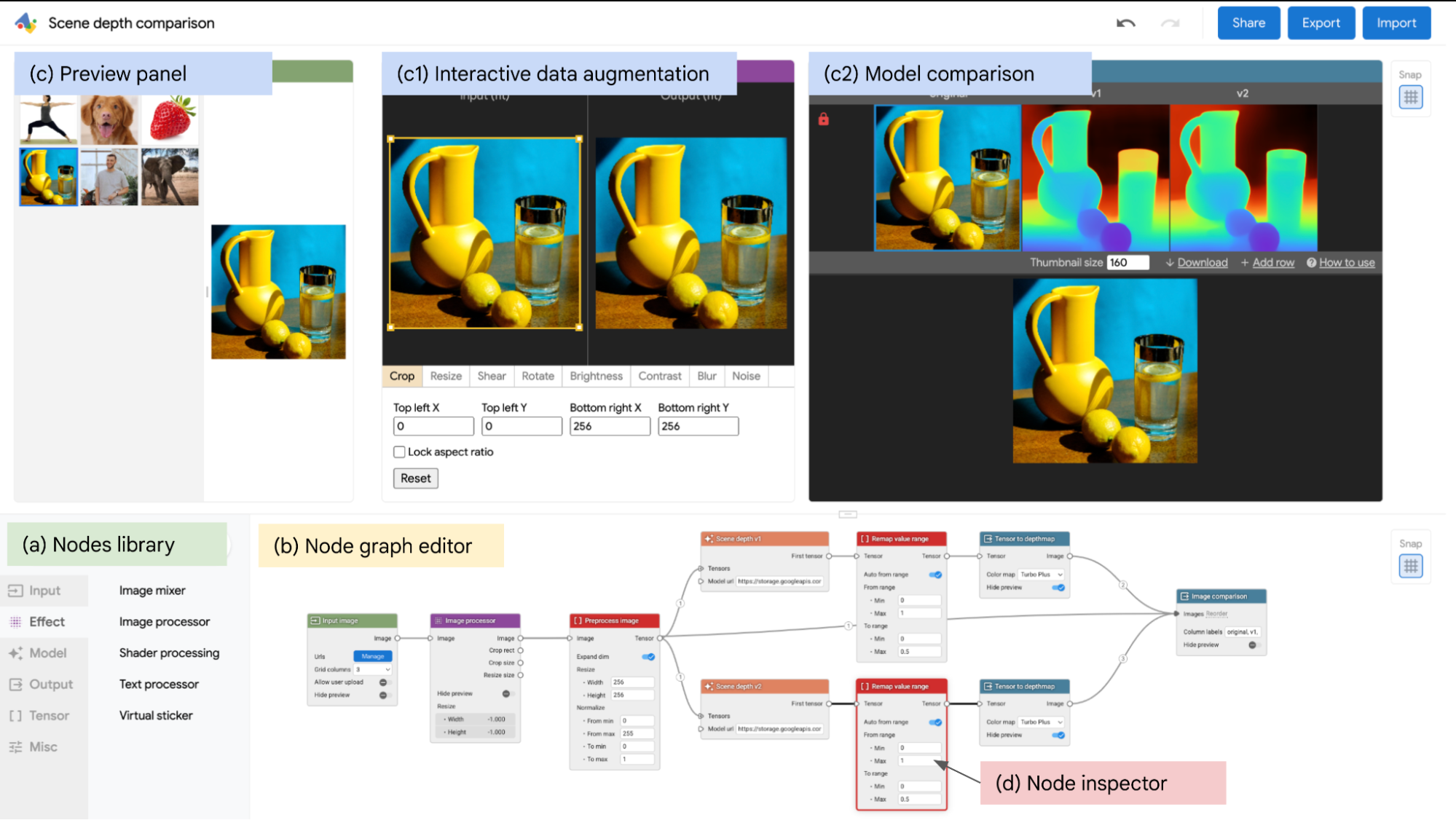 |
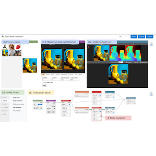
| The visual programming interface allows users to quickly develop and evaluate ML models by composing and previewing node-graphs with real-time results. |
Over the last year, we’ve been iteratively designing and improving the Visual Blocks platform. Weekly feedback sessions with the three ML teams from the formative study showed appreciation for the platform’s unique capabilities and its potential to accelerate ML prototyping through:
To evaluate the usability and effectiveness of Visual Blocks, we conducted four case studies with 15 ML practitioners. They used the platform to prototype different multimedia applications: portrait depth with relighting effects, scene depth with visual effects, alpha matting for virtual conferences, and audio denoising for communication.
 |
| The system streamlining comparison of two Portrait Depth models, including customized visualization and effects. |
With a short introduction and video tutorial, participants were able to quickly identify differences between the models and select a better model for their use case. We found that Visual Blocks helped facilitate rapid and deeper understanding of model benefits and trade-offs:
“It gives me intuition about which data augmentation operations that my model is more sensitive [to], then I can go back to my training pipeline, maybe increase the amount of data augmentation for those specific steps that are making my model more sensitive.” (Participant 13)
“It’s a fair amount of work to add some background noise, I have a script, but then every time I have to find that script and modify it. I’ve always done this in a one-off way. It’s simple but also very time consuming. This is very convenient.” (Participant 15)
 |
| The system allows researchers to compare multiple Portrait Depth models at different noise levels, helping ML practitioners identify the strengths and weaknesses of each. |
In a post-hoc survey using a seven-point Likert scale, participants reported Visual Blocks to be more transparent about how it arrives at its final results than Colab (Visual Blocks 6.13 ± 0.88 vs. Colab 5.0 ± 0.88, 𝑝 < .005) and more collaborative with users to come up with the outputs (Visual Blocks 5.73 ± 1.23 vs. Colab 4.15 ± 1.43, 𝑝 < .005). Although Colab assisted users in thinking through the task and controlling the pipeline more effectively through programming, Users reported that they were able to complete tasks in Visual Blocks in just a few minutes that could normally take up to an hour or more. For example, after watching a 4-minute tutorial video, all participants were able to build a custom pipeline in Visual Blocks from scratch within 15 minutes (10.72 ± 2.14). Participants usually spent less than five minutes (3.98 ± 1.95) getting the initial results, then were trying out different input and output for the pipeline.
 |
| User ratings between Rapsai (initial prototype of Visual Blocks) and Colab across five dimensions. |
More results in our paper showed that Visual Blocks helped participants accelerate their workflow, make more informed decisions about model selection and tuning, analyze strengths and weaknesses of different models, and holistically evaluate model behavior with real-world input.
Visual Blocks lowers development barriers for ML-based multimedia applications. It empowers users to experiment without worrying about coding or technical details. It also facilitates collaboration between designers and developers by providing a common language for describing ML pipelines. In the future, we plan to open this framework up for the community to contribute their own nodes and integrate it into many different platforms. We expect visual programming for machine learning to be a common interface across ML tooling going forward.
This work is a collaboration across multiple teams at Google. Key contributors to the project include Ruofei Du, Na Li, Jing Jin, Michelle Carney, Xiuxiu Yuan, Kristen Wright, Mark Sherwood, Jason Mayes, Lin Chen, Jun Jiang, Scott Miles, Maria Kleiner, Yinda Zhang, Anuva Kulkarni, Xingyu “Bruce” Liu, Ahmed Sabie, Sergio Escolano, Abhishek Kar, Ping Yu, Ram Iyengar, Adarsh Kowdle, and Alex Olwal.
We would like to extend our thanks to Jun Zhang and Satya Amarapalli for a few early-stage prototypes, and Sarah Heimlich for serving as a 20% program manager, Sean Fanello, Danhang Tang, Stephanie Debats, Walter Korman, Anne Menini, Joe Moran, Eric Turner, and Shahram Izadi for providing initial feedback for the manuscript and the blog post. We would also like to thank our CHI 2023 reviewers for their insightful feedback.
Batch inference is a common pattern where prediction requests are batched together on input, a job runs to process those requests against a trained model, and the output includes batch prediction responses that can then be consumed by other applications or business functions. Running batch use cases in production environments requires a repeatable process for model retraining as well as batch inference. That process should also include monitoring that model to measure performance over time.
In this post, we show how to create repeatable pipelines for your batch use cases using Amazon SageMaker Pipelines, Amazon SageMaker model registry, SageMaker batch transform jobs, and Amazon SageMaker Model Monitor. This solution highlights the ability to use the fully managed features within SageMaker MLOps to reduce operational overhead through fully managed and integrated capabilities.
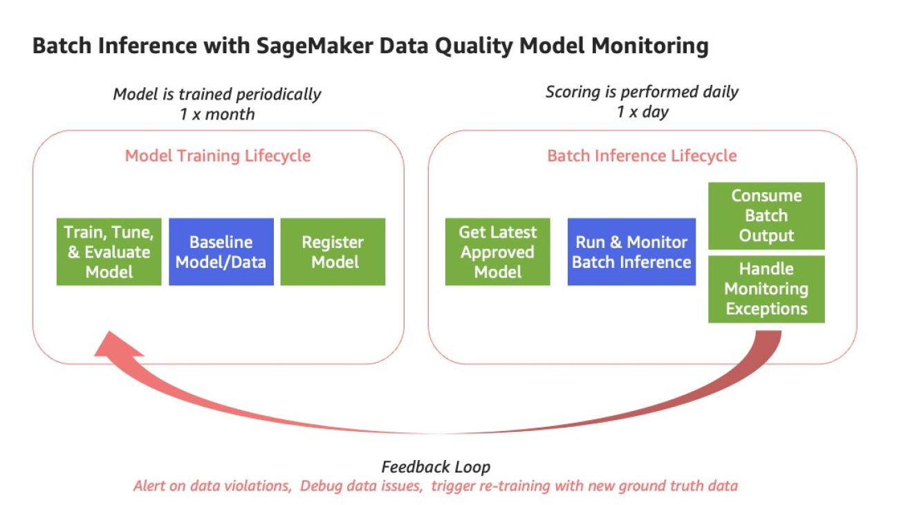
There are multiple scenarios for performing batch inference. In some cases, you may be retraining your model every time you run batch inference. Alternatively, you may be training your model less frequently than you are performing batch inference. In this post, we focus on the second scenario. For this example, let’s assume you have a model that is trained periodically, roughly one time per month. However, batch inference is performed against the latest model version on a daily basis. This is a common scenario, in which the model training lifecycle is different than the batch inference lifecycle.
The architecture supporting the introduced batch scenario contains two separate SageMaker pipelines, as shown in the following diagram.

We use the first pipeline to train the model and baseline the training data. We use the generated baseline for ongoing monitoring in the second pipeline. The first pipeline includes the steps needed to prepare data, train the model, and evaluate the performance of the model. If the model performs acceptably according to the evaluation criteria, the pipeline continues with a step to baseline the data using a built-in SageMaker Pipelines step. For the data drift Model Monitor type, the baselining step uses a SageMaker managed container image to generate statistics and constraints based on your training data. This baseline is then used to monitor for signals of data drift during batch inference. Finally, the first pipeline completes when a new model version is registered into the SageMaker model registry. At this point, the model can be approved automatically, or a secondary manual approval can be required based on a peer review of model performance and any other identified criteria.
In the second pipeline, the first step queries the model registry for the latest approved model version and runs the data monitoring job, which compares the data baseline generated from the first pipeline with the current input data. The final step in the pipeline is performing batch inference against the latest approved model.
The following diagram illustrates the solution architecture for each pipeline.

For our dataset, we use a synthetic dataset from a telecommunications mobile phone carrier. This sample dataset contains 5,000 records, where each record uses 21 attributes to describe the customer profile. The last attribute, Churn, is the attribute that we want the ML model to predict. The target attribute is binary, meaning the model predicts the output as one of two categories (True or False).
The following GitHub repo contains the code for demonstrating the steps performed in each pipeline. It contains three notebooks: to perform the initial setup, to create the model train and baseline pipeline, and create the batch inference and Model Monitor pipeline. The repository also includes additional Python source code with helper functions, used in the setup notebook, to set up required permissions.
The following screenshot lists some permission policies that are required by the SageMaker execution role for the workflow. You can enable these permission policies through AWS Identity and Access Management (IAM) role permissions.

AmazonSageMaker-ExecutionPolicy-<...> is the execution role associated with the SageMaker user and has the necessary Amazon Simple Storage Service (Amazon S3) bucket policies. Custom_IAM_roles_policy and Custom_Lambda_policy are two custom policies created to support the required actions for the AWS Lambda function. To add the two custom policies, go to the appropriate role (associated with your SageMaker user) in IAM, click on Add permissions and then Create inline policy. Then, choose JSON inside Create policy, add the policy code for first custom policy and save the policy. Repeat the same for the second custom policy.
0.Setup.ipynb is a prerequisite notebook required before running notebooks 1 and 2. The code sets up the S3 paths for pipeline inputs, outputs, and model artifacts, and uploads scripts used within the pipeline steps. This notebook also uses one of the provided helper functions, create_lambda_role, to create a Lambda role that is used in notebook 2, 2.SageMakerPipeline-ModelMonitoring-DataQuality-BatchTransform.ipynb. See the following code:
After you’ve successfully completed all of the tasks in the setup notebook, you’re ready to build the first pipeline to train and baseline the model.
In this section, we take a deep dive into the SageMaker pipeline used to train and baseline the model. The necessary steps and code are in the 1.SageMakerPipeline-BaselineData-Train.ipynb notebook. This pipeline takes the raw customer churn data as input, and then performs the steps required to prepare the data, train the model, evaluate the model, baseline the model, and register the model in the model registry.

To build a SageMaker pipeline, you configure the underlying job (such as SageMaker Processing), configure the pipeline steps to run the job, and then configure and run the pipeline. We complete the following steps:
The model build pipeline is a three-step process:

To prepare the data, we configure a data processing step. This step runs a SageMaker Processing job, using the built-in ProcessingStep, to prepare the raw data on input for training and evaluation.
To train the model, we configure a training job step. This step runs a SageMaker Training job, using the built-in TrainingStep. For this use case, we perform binary classification using XGBoost. The output of this step is a model artifact, model.tar.gz, stored in Amazon S3.
The last step is responsible for evaluating model performance using the test holdout dataset. This step uses the built-in ProcessingStep with the provided code, evaluation.py, to evaluate performance metrics (accuracy, area under curve).
To monitor the model and data, a baseline is required.

Monitoring for data drift requires a baseline of training data. The baseline step uses Pipelines’ built-in QualityCheckStep. This step automatically runs a SageMaker Processing job that uses the Model Monitor pre-built container image. We use this same container image for the baselining as well as the model monitoring; however, the parameters used during configuration of this step direct the appropriate behavior. In this case, we are baselining the data, so we need to ensure that the quality_check_config parameter is using DataQualityCheckConfig, which identifies the S3 input and output paths. We’re also setting register_new_baseline and skip_check to true. When these values are both set to true, it tells SageMaker to run this step as a baseline job and create a new baseline. To get a better understanding of the parameters that control the behavior of the SageMaker pre-built container image, refer to Baseline calculation, drift detection and lifecycle with ClarifyCheck and QualityCheck steps in Amazon SageMaker Model Building Pipelines.
See the following code:
This step generates two JSON files as output:
These constraints can also be modified and are used to detect signals of drift during model monitoring.
Next, we configure the steps to package for deployment and register the model in the model registry using two additional pipeline steps.

The package model step packages the model for use with the SageMaker batch transform deployment option. model.create() creates a model entity, which will be included in the custom metadata registered for this model version and later used in the second pipeline for batch inference and model monitoring. See the following code:
The register model step registers the model version and associated metadata to the SageMaker model registry. This includes model performance metrics as well as metadata for the data drift baseline, including the Amazon S3 locations of the statistics and constraints files produced through the baselining step. You’ll also notice the additional custom metadata noted customer_metadata_properties pulling the model entity information that will be used later in the inference pipeline. The ability to provide custom metadata within the model registry is a great way to incorporate additional metadata that should be collected that isn’t explicitly defined in native SageMaker parameters. See the following code:
The conditional step, ConditionStep, compares model accuracy against an identified threshold and checks the quality of the trained model.

It reads the evaluation.json file and checks if the model accuracy, or whatever objective metric you are optimizing for, meets the criteria you’ve defined. In this case, the criteria is defined using one of the built-in conditions, ConditionGreaterThanOrEqualTo. If the condition is satisfied, the pipeline continues to baseline the data and perform subsequent steps in the pipeline. The pipeline stops if the condition is not met. Because the condition explicitly calls out the next steps in the pipeline, we have to ensure those steps are configured prior to configuring our conditional step. See the following code:
At this point, all the steps of the train and baseline pipeline are defined and configured. Now it’s time to define, create, and start the pipeline.

First, we define the pipeline, Pipeline(), providing a pipeline name and a list of steps previously configured to include in the pipeline. Next, we create the pipeline using training_pipeline.upsert(). Finally, we start the pipeline using training_pipeline.start(). See the following code:
When the pipeline starts running, you can visualize its status on Studio. The following diagram shows which steps from the pipeline process relate to the steps of the pipeline directed acyclic graph (DAG). After the train and baseline pipeline run successfully, it registers the trained model as part of the model group in the model registry. The pipeline is currently set up to register the model in a Pending state, which requires a manual approval. Optionally, you can configure the model registration step to automatically approve the model in the model registry. The second pipeline will pull the latest approved model from the registry for inference.

In Studio, you can choose any step to see its key metadata. As an example, the data quality check step (baseline step) within the pipeline DAG shows the S3 output locations of statistics.json and constraints.json in the Reports section. These are key files calculated from raw data used as a baseline.

After the pipeline has run, the baseline (statistics and constraints) for data quality monitoring can be inspected, as shown in the following screenshots.


In this section, we dive into the second pipeline used for monitoring the new batch input data for signals of data drift and running batch inference using SageMaker Pipelines. The necessary steps and code are within 2.SageMakerPipeline-ModelMonitoring-DataQuality-BatchTransform.ipynb. This pipeline includes the following steps:

Before we start the model monitoring and batch transform job, we need to query the model registry to get the latest approved model that we will use for batch inference.

To do this, we use a Lambda step, which allows us to include custom logic within our pipeline. The lambda_getapproved_model.py Lambda function queries the SageMaker model registry for a specific model package group provided on input to identify the latest approved model version and return related metadata. The output includes metadata created from our first pipeline:
The output is then used as input in the next step in the pipeline, which performs batch monitoring and scoring using the latest approved model.
To create and run the Lambda function as part of the SageMaker pipeline, we need to add the function as a LambdaStep in the pipeline:
After we create the Lambda step to get the latest approved model, we can create the MonitorBatchTransformStep. This native step orchestrates and manages two child tasks that are run in succession. The first task includes the Model Monitor job that runs a Processing job using a built-in container image used to monitor the batch input data and compare it against the constraints from the previously generated baseline from Pipeline 1. In addition, this step kicks off the batch transform job, which processes the input data against the latest approved model in the model registry.

This batch deployment and data quality monitoring step takes the S3 URI of the batch prediction input data on input. This is parameterized to allow for each run of the pipeline to include a new input dataset. See the following code:
Next, we need to configure the transformer for the batch transform job that will process the batch prediction requests. In the following code, we pass in the model name that was pulled from the custom metadata of the model registry, along with other required parameters:
The data quality monitor accepts the S3 URI of the baseline statistics and constraints for the latest approved model version from the model registry to run the data quality monitoring job during the pipeline run. This job compares the batch prediction input data with the baseline data to identify any violations signaling potential data drift. See the following code:
Next, we use MonitorBatchTransformStep to run and monitor the transform job. This step runs a batch transform job using the transformer object we configured and monitors the data passed to the transformer before running the job.
Optionally, you can configure the step to fail if a violation to data quality is found by setting the fail_on_violation flag to False.
See the following code:
After we define the LambdaStep and MonitorBatchTransformStep, we can create the SageMaker pipeline.

See the following code:
We can now use the upsert() method, which will create or update the SageMaker pipeline with the configuration we specified:
Although there are multiple ways to start a SageMaker pipeline, when the pipeline has been created, we can run the pipeline using the start() method.
Note that in order for the LambdaStep to successfully retrieve an approved model, the model that was registered as part of Pipeline 1 needs to have an Approved status. This can be done in Studio or using Boto3. Refer to Update the Approval Status of a Model for more information.

To run the SageMaker pipeline on a schedule or based on an event, refer to Schedule a Pipeline with Amazon EventBridge.
Model Monitor uses a SageMaker Processing job that runs the DataQuality check using the baseline statistics and constraints. The DataQuality Processing job emits a violations report to Amazon S3 and also emits log data to Amazon CloudWatch Logs under the log group for the corresponding Processing job. Sample code for querying Amazon CloudWatch logs is provided in the notebook.

We’ve now walked you through how to create the first pipeline for model training and baselining, as well as the second pipeline for performing batch inference and model monitoring. This allows you to automate both pipelines while incorporating the different lifecycles between training and inference.
To further mature this reference pattern, you can identify a strategy for feedback loops, providing awareness and visibility of potential signals of drift across key stakeholders. At a minimum, it’s recommended to automate exception handling by filtering logs and creating alarms. These alarms may need additional analysis by a data scientist, or you can implement additional automation supporting an automatic retraining strategy using new ground truth data by integrating the model training and baselining pipeline with Amazon EventBridge. For more information, refer to Amazon EventBridge Integration.

After you run the baseline and batch monitoring pipelines, make sure to clean up any resources that won’t be utilized, either programmatically via the SageMaker console, or through Studio. In addition, delete the data in Amazon S3, and make sure to stop any Studio notebook instances to not incur any further charges.
In this post, you learned how to create a solution for a batch model that is trained less frequently than batch inference is performed against that trained model using SageMaker MLOps features, including Pipelines, the model registry, and Model Monitor. To expand this solution, you could incorporate this into a custom SageMaker project that also incorporates CI/CD and automated triggers using standardized MLOps templates. To dive deeper into the solution and code shown in this demo, check out the GitHub repo. Also, refer to Amazon SageMaker for MLOps for examples related to implementing MLOps practices with SageMaker.
 Shelbee Eigenbrode is a Principal AI and Machine Learning Specialist Solutions Architect at Amazon Web Services (AWS). She has been in technology for 24 years spanning multiple industries, technologies, and roles. She is currently focusing on combining her DevOps and ML background into the domain of MLOps to help customers deliver and manage ML workloads at scale. With over 35 patents granted across various technology domains, she has a passion for continuous innovation and using data to drive business outcomes. Shelbee is a co-creator and instructor of the Practical Data Science specialization on Coursera. She is also the Co-Director of Women In Big Data (WiBD), Denver chapter. In her spare time, she likes to spend time with her family, friends, and overactive dogs.
 Sovik Kumar Nath is an AI/ML solution architect with AWS. He has experience in designs and solutions for machine learning, business analytics within financial, operational, and marketing analytics; healthcare; supply chain; and IoT. Outside work, Sovik enjoys traveling and watching movies.
 Marc Karp is a ML Architect with the Amazon SageMaker Service team. He focuses on helping customers design, deploy, and manage ML workloads at scale. In his spare time, he enjoys traveling and exploring new places.

Content creators using Epic Games’ open, advanced real-time 3D creation tool, Unreal Engine, are now equipped with more features to bring their work to life with NVIDIA Omniverse, a platform for creating and operating metaverse applications.
The Omniverse Connector for Unreal Engine’s 201.0 update brings significant enhancements to creative workflows using both open platforms.
The Unreal Engine Omniverse Connector 201.0 release delivers improvements in import, export and live workflows, as well as updated software development kits.
New features include:
Artists and game content creators are seeing notable improvements to their workflows thanks to this connector update.
Developer and creator Abdelrazik Maghata, aka MR GFX on YouTube, recently joined an Omniverse livestream to demonstrate his workflow using Unreal Engine and Omniverse. Maghata explained how to animate a character in real time by connecting the Omniverse Audio2Face generative AI-powered application to Epic’s MetaHuman framework in Unreal Engine.
Maghata, who’s been a content creator on YouTube for 15 years, uses his platform to teach others about the benefits of Unreal Engine for their 3D workflows. He’s recently added Omniverse into his repertoire to build connections between his favorite content creation tools.
“Omniverse will transform the world of 3D,” he said.
Omniverse ambassador and short-film phenom Jae Solina often uses the Unreal Engine Connector in his creative process, as well. The connector has greatly improved his workflow efficiency and increased productivity by providing interoperability between his favorite tools, Solina said.
Getting connected is simple. Learn how to accelerate creative workflows with the Unreal Engine Omniverse Connector by watching this video:
At the recent NVIDIA GTC conference, the Omniverse team hosted many sessions spotlighting how creators can enhance their workflows with generative AI, 3D SimReady assets and more. Watch for free on demand.
Plus, join the latest Omniverse community challenge, running through the end of the month. Use the Unreal Engine Omniverse Connector and share your creation — whether it’s fan art, a video-game character or even an original game — on social media using the hashtag #GameArtChallenge for a chance to be featured on channels for NVIDIA Omniverse (Twitter, LinkedIn, Instagram) and NVIDIA Studio (Twitter, Facebook, Instagram).
Are you up for a challenge?
From now until April 30, share your video-game inspired work in our #GameArtChallenge.
@rafianimates is making his very own #AR game and shared some WIPs of the characters #MadeInOmniverse with @VoxEdit & #MagicaVoxel. pic.twitter.com/pppDNarNk4
— NVIDIA Omniverse (@nvidiaomniverse) March 9, 2023
Get started with NVIDIA Omniverse by downloading the standard license free, or learn how Omniverse Enterprise can connect teams. Developers can get started with these Omniverse resources.
To stay up to date on the platform, subscribe to the newsletter and follow NVIDIA Omniverse on Instagram, Medium and Twitter. Check out the Omniverse forums, Discord server, Twitch and YouTube channels.
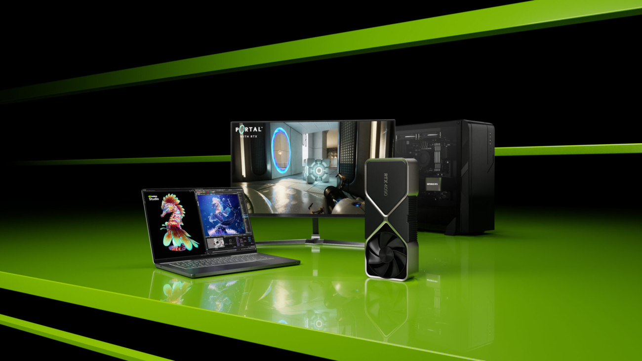
What’s the difference between NVIDIA GeForce RTX 30 and 40 Series GPUs for gamers?
To briefly set aside the technical specifications, the difference lies in the level of performance and capability each series offers.
Both deliver great graphics. Both offer advanced new features driven by NVIDIA’s global AI revolution a decade ago. Either can power glorious high-def gaming experiences.
But the RTX 40 Series takes everything RTX GPUs deliver and turns it up to 11.
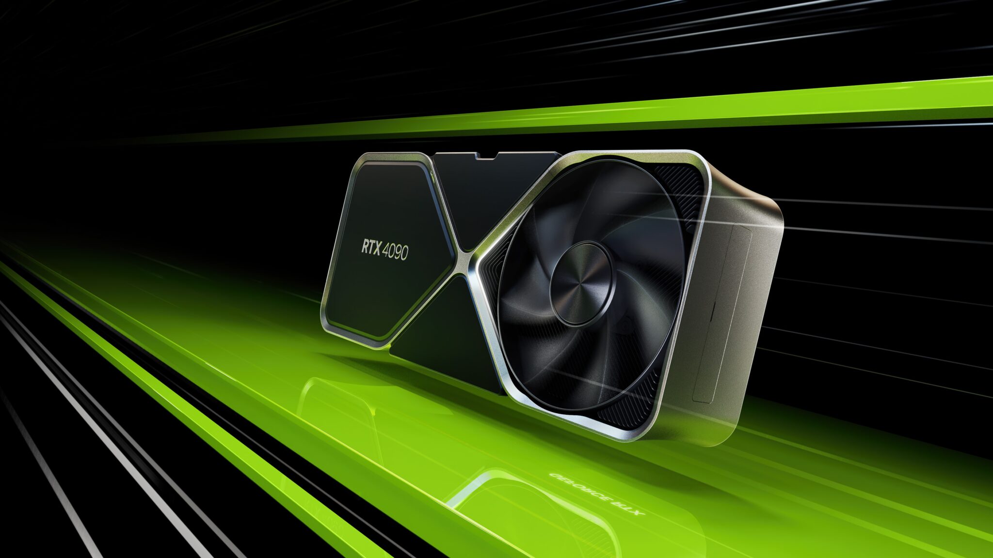
“Think of any current PC gaming workload that includes ‘future-proofed’ overkill settings, then imagine the RTX 4090 making like Grave Digger and crushing those tests like abandoned cars at a monster truck rally,” writes Ars Technica.
That said, the RTX 30 Series and 40 Series GPUs have a lot in common.
Both offer hardware-accelerated ray tracing thanks to specialized RT Cores. They also have AI-enabling Tensor Cores that supercharge graphics. And both come loaded with support for next-generation AI and rendering technologies.
But NVIDIA’s GeForce RTX 40 Series delivers all this in a simply unmatched way.
Unveiled in September 2022, the RTX 40 Series GPUs consist of four variations: the RTX 4090, RTX 4080, RTX 4070 Ti and RTX 4070.
All four are built on NVIDIA’s Ada Lovelace architecture, a significant upgrade over the NVIDIA Ampere architecture used in the RTX 30 Series GPUs.
While both 30 Series and 40 Series GPUs utilize Tensor Cores, Ada’s new fourth-generation Tensor Cores are unbelievably fast, increasing throughput by up to 5x, to 1.4 Tensor-petaflops using the new FP8 Transformer Engine, first introduced in NVIDIA’s Hopper architecture H100 data center GPU.
NVIDIA made real-time ray tracing a reality with the invention of RT Cores, dedicated processing cores on the GPU designed to tackle performance-intensive ray-tracing workloads.
Stay updated on the latest news, features, and tips for gaming, creating, and streaming with NVIDIA GeForce; check out GeForce News – the ultimate destination for GeForce enthusiasts.
Advanced ray tracing requires computing the impact of many rays striking numerous different material types throughout a scene, creating a sequence of divergent, inefficient workloads for the shaders to calculate the appropriate levels of light, darkness and color while rendering a 3D scene.
Ada’s third-generation RT Cores have up to twice the ray-triangle intersection throughput, increasing RT-TFLOP performance by over 2x vs. Ampere’s best.
And Ada’s new Shader Execution Reordering technology dynamically reorganizes these previously inefficient workloads into considerably more efficient ones. SER can improve shader performance for ray-tracing operations by up to 3x and in-game frame rates by up to 25%.
As a result, 40 Series GPUs excel at real-time ray tracing, delivering unmatched gameplay on the most demanding titles, such as Cyberpunk 2077 that support the technology.
Ada also advances NVIDIA DLSS, which brings advanced deep learning techniques to graphics, massively boosting performance.
Powered by the new fourth-gen Tensor Cores and Optical Flow Accelerator on GeForce RTX 40 Series GPUs, DLSS 3 uses AI to create additional high-quality frames.
As a result, RTX 40 Series GPUs deliver buttery-smooth gameplay in the latest and greatest PC games.
NVIDIA GeForce RTX 40 Series graphics cards also feature new eighth-generation NVENC (NVIDIA Encoders) with AV1 encoding, enabling new possibilities for streamers, broadcasters, video callers and creators.
AV1 is 40% more efficient than H.264. This allows users streaming at 1080p to increase their stream resolution to 1440p while running at the same bitrate and quality.
Remote workers will be able to communicate more smoothly with colleagues and clients. For creators, the ability to stream high-quality video with reduced bandwidth requirements can enable smoother collaboration and content delivery, allowing for a more efficient creative process.
RTX 40 Series GPUs are also built at the absolute cutting edge, with a custom TSMC 4N process. The process and Ada architecture are ultra-efficient.
And RTX 40 Series GPUs come loaded with the memory needed to keep its Ada GPUs running at full tilt.
All that said, RTX 30 Series GPUs remain powerful and popular.
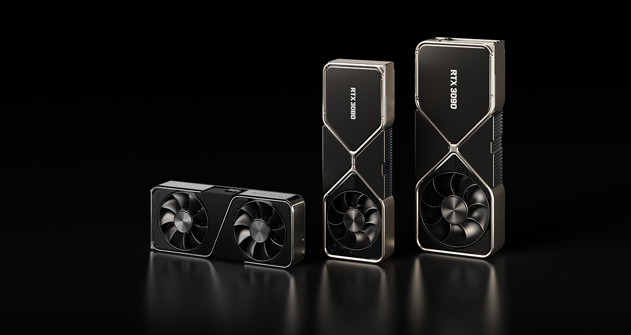
Launched in September 2020, the RTX 30 Series GPUs include a range of different models, from the RTX 3050 to the RTX 3090 Ti.
All deliver the grunt to run the latest games in high definition and at smooth frame rates.
But while the RTX 30 Series GPUs have remained a popular choice for gamers and professionals since their release, the RTX 40 Series GPUs offer significant improvements for gamers and creators alike, particularly those who want to crank up settings with high frames rates, drive big 4K displays, or deliver buttery-smooth streaming to global audiences.
With higher performance, enhanced ray-tracing capabilities, support for DLSS 3 and better power efficiency, the RTX 40 Series GPUs are an attractive option for those who want the latest and greatest technology.

 Bard can now help with programming and software development tasks, across more than 20 programming languages.Read More
Time-series forecasting is an important research area that is critical to several scientific and industrial applications, like retail supply chain optimization, energy and traffic prediction, and weather forecasting. In retail use cases, for example, it has been observed that improving demand forecasting accuracy can meaningfully reduce inventory costs and increase revenue.
Modern time-series applications can involve forecasting hundreds of thousands of correlated time-series (e.g., demands of different products for a retailer) over long horizons (e.g., a quarter or year away at daily granularity). As such, time-series forecasting models need to satisfy the following key criterias:
A number of neural network–based solutions have been able to show good performance on benchmarks and also support the above criterion. However, these methods are typically slow to train and can be expensive for inference, especially for longer horizons.
In “Long-term Forecasting with TiDE: Time-series Dense Encoder”, we present an all multilayer perceptron (MLP) encoder-decoder architecture for time-series forecasting that achieves superior performance on long horizon time-series forecasting benchmarks when compared to transformer-based solutions, while being 5–10x faster. Then in “On the benefits of maximum likelihood estimation for Regression and Forecasting”, we demonstrate that using a carefully designed training loss function based on maximum likelihood estimation (MLE) can be effective in handling different data modalities. These two works are complementary and can be applied as a part of the same model. In fact, they will be available soon in Google Cloud AI’s Vertex AutoML Forecasting.
Deep learning has shown promise in time-series forecasting, outperforming traditional statistical methods, especially for large multivariate datasets. After the success of transformers in natural language processing (NLP), there have been several works evaluating variants of the Transformer architecture for long horizon (the amount of time into the future) forecasting, such as FEDformer and PatchTST. However, other work has suggested that even linear models can outperform these transformer variants on time-series benchmarks. Nonetheless, simple linear models are not expressive enough to handle auxiliary features (e.g., holiday features and promotions for retail demand forecasting) and non-linear dependencies on the past.
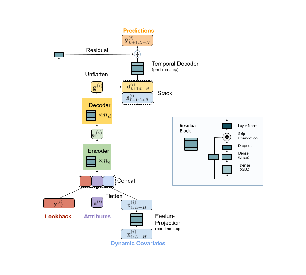
We present a scalable MLP-based encoder-decoder model for fast and accurate multi-step forecasting. Our model encodes the past of a time-series and all available features using an MLP encoder. Subsequently, the encoding is combined with future features using an MLP decoder to yield future predictions. The architecture is illustrated below.
 |
| TiDE model architecture for multi-step forecasting. |
TiDE is more than 10x faster in training compared to transformer-based baselines while being more accurate on benchmarks. Similar gains can be observed in inference as it only scales linearly with the length of the context (the number of time-steps the model looks back) and the prediction horizon. Below on the left, we show that our model can be 10.6% better than the best transformer-based baseline (PatchTST) on a popular traffic forecasting benchmark, in terms of test mean squared error (MSE). On the right, we show that at the same time our model can have much faster inference latency than PatchTST.
 |
| Left: MSE on the test set of a popular traffic forecasting benchmark. Right: inference time of TiDE and PatchTST as a function of the look-back length. |
Our research demonstrates that we can take advantage of MLP’s linear computational scaling with look-back and horizon sizes without sacrificing accuracy, while transformers scale quadratically in this situation.
In most forecasting applications the end user is interested in popular target metrics like the mean absolute percentage error (MAPE), weighted absolute percentage error (WAPE), etc. In such scenarios, the standard approach is to use the same target metric as the loss function while training. In “On the benefits of maximum likelihood estimation for Regression and Forecasting”, accepted at ICLR, we show that this approach might not always be the best. Instead, we advocate using the maximum likelihood loss for a carefully chosen family of distributions (discussed more below) that can capture inductive biases of the dataset during training. In other words, instead of directly outputting point predictions that minimize the target metric, the forecasting neural network predicts the parameters of a distribution in the chosen family that best explains the target data. At inference time, we can predict the statistic from the learned predictive distribution that minimizes the target metric of interest (e.g., the mean minimizes the MSE target metric while the median minimizes the WAPE). Further, we can also easily obtain uncertainty estimates of our forecasts, i.e., we can provide quantile forecasts by estimating the quantiles of the predictive distribution. In several use cases, accurate quantiles are vital, for instance, in demand forecasting a retailer might want to stock for the 90th percentile to guard against worst-case scenarios and avoid lost revenue.
The choice of the distribution family is crucial in such cases. For example, in the context of sparse count data, we might want to have a distribution family that can put more probability on zero, which is commonly known as zero-inflation. We propose a mixture of different distributions with learned mixture weights that can adapt to different data modalities. In the paper, we show that using a mixture of zero and multiple negative binomial distributions works well in a variety of settings as it can adapt to sparsity, multiple modalities, count data, and data with sub-exponential tails.
 |
| A mixture of zero and two negative binomial distributions. The weights of the three components, a1, a2 and a3, can be learned during training. |
We use this loss function for training Vertex AutoML models on the M5 forecasting competition dataset and show that this simple change can lead to a 6% gain and outperform other benchmarks in the competition metric, weighted root mean squared scaled error (WRMSSE).
| M5 Forecasting | WRMSSE |
| Vertex AutoML | 0.639 +/- 0.007 |
| Vertex AutoML with probabilistic loss | 0.581 +/- 0.007 |
| DeepAR | 0.789 +/- 0.025 |
| FEDFormer | 0.804 +/- 0.033 |
We have shown how TiDE, together with probabilistic loss functions, enables fast and accurate forecasting that automatically adapts to different data distributions and modalities and also provides uncertainty estimates for its predictions. It provides state-of-the-art accuracy among neural network–based solutions at a fraction of the cost of previous transformer-based forecasting architectures, for large-scale enterprise forecasting applications. We hope this work will also spur interest in revisiting (both theoretically and empirically) MLP-based deep time-series forecasting models.
This work is the result of a collaboration between several individuals across Google Research and Google Cloud, including (in alphabetical order): Pranjal Awasthi, Dawei Jia, Weihao Kong, Andrew Leach, Shaan Mathur, Petros Mol, Shuxin Nie, Ananda Theertha Suresh, and Rose Yu.
