Monthly Archives: April 2023

In the world of machine learning (ML), the quality of the dataset is of significant importance to model predictability. Although more data is usually better, large datasets with a high number of features can sometimes lead to non-optimal model performance due to the curse of dimensionality. Analysts can spend a significant amount of time transforming data to improve model performance. Additionally, large datasets are costlier and take longer to train. If time is a constraint, model performance may be limited as a result.

Dimension reduction techniques can help reduce the size of your data while maintaining its information, resulting in quicker training times, lower cost, and potentially higher-performing models.

Amazon SageMaker Data Wrangler is a purpose-built data aggregation and preparation tool for ML. Data Wrangler simplifies the process of data preparation and feature engineering like data selection, cleansing, exploration, and visualization from a single visual interface. Data Wrangler has more than 300 preconfigured data transformations that can effectively be used in transforming the data. In addition, you can write custom transformation in PySpark, SQL, and pandas.

Today, we’re excited to add a new transformation technique that is commonly used in the ML world to the list of Data Wrangler pre-built transformations: dimensionality reduction using Principal Component Analysis. With this new feature, you can reduce the high number of dimensions in your datasets to one that can be used with popular ML algorithms with just a few clicks on the Data Wrangler console. This can have significant improvements in your model performance with minimal effort.

In this post, we provide an overview of this new feature and show how to use it in your data transformation. We will show how to use dimensionality reduction on large sparse datasets.

Overview of Principal Component Analysis

Principal Component Analysis (PCA) is a method by which the dimensionality of features can be transformed in a dataset with many numerical features into one with fewer features while still retaining as much information as possible from the original dataset. This is done by finding a new set of features called components, which are composites of the original features that are uncorrelated with one another. Several features in a dataset often have less impact on the final result and may increase the processing time of ML models. It can become difficult for humans to understand and solve such high-dimensional problems. Dimensionality reduction techniques like PCA can help solve this for us.

Solution overview

In this post, we show how you can use the dimensionality reduction transform in Data Wrangler on the MNIST dataset to reduce the number of features by 85% and still achieve similar or better accuracy than the original dataset. The MNIST (Modified National Institute of Standards and Technology) dataset, which is the de facto “hello world” dataset in computer vision, is a dataset of handwritten images. Each row of the dataset corresponds to a single image that is 28 x 28 pixels, for a total of 784 pixels. Each pixel is represented by a single feature in the dataset with a pixel value ranging from 0–255.

To learn more about the new dimensionality reduction feature, refer to Reduce Dimensionality within a Dataset.

Prerequisites

This post assumes that you have an Amazon SageMaker Studio domain set up. For details on how to set it up, refer to Onboard to Amazon SageMaker Domain Using Quick setup.

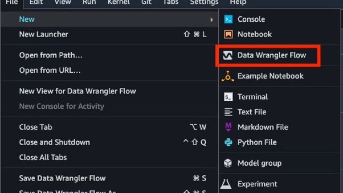
To get started with the new capabilities of Data Wrangler, open Studio after upgrading to the latest release and choose the File menu, New, and Flow, or choose New data flow from the Studio launcher.

Perform a Quick Model analysis

The dataset we use in this post contains 60,000 training examples and labels. Each row consists of 785 values: the first value is the label (a number from 0–9) and the remaining 784 values are the pixel values (a number from 0–255). First, we perform a Quick Model analysis on the raw data to get performance metrics and compare them with the model metrics post-PCA transformations for evaluation. Complete the following steps:

1. Download the MNIST dataset training dataset.
2. Extract the data from the .zip file and upload into an Amazon Simple Storage Service (Amazon S3) bucket.
3. In Studio, choose New and Data Wrangler Flow to create a new Data Wrangler flow.
   
4. Choose Import data to load the data from Amazon S3.
   
5. Choose Amazon S3 as your data source.
   
6. Select the dataset uploaded to your S3 bucket.
7. Leave the default settings and choose Import.
   

After the data is imported, Data Wrangler automatically validates the datasets and detects the data types for all the columns based on its sampling. In the MNIST dataset, because all the columns are long, we leave this step as is and go back to the data flow.

8. Choose Data flow at the top of the Data types page to return to the main data flow.
   

The flow editor now shows two blocks showcasing that the data was imported from a source and the data types recognized. You can also edit the data types if needed.

After confirming that the data quality is acceptable, we go back to the data flow and use Data Wrangler’s Data Quality and Insights Report. This report performs an analysis on the imported dataset and provides information about missing values, outliers, target leakage, imbalanced data, and a Quick Model analysis. Refer to Get Insights On Data and Data Quality for more information.

For this analysis, we only focus on the Quick Model part of the Data Quality report.

9. Choose the plus sign next to Data types, then choose Add analysis.
   
10. For Analysis type¸ choose Data Quality And Insights Report.
11. For Target column, choose label.
12. For Problem type, select Classification (this step is optional).
13. Choose Create.
    

For this post, we use the Data Quality and Insights Report to show how the model performance is mostly preserved using PCA. We recommend that you use a deep learning-based approach for better performance.

The following screenshot shows a summary of the dataset from the report. Fortunately, we don’t have any missing values. The time taken for the report to generate depends on the size of the dataset, number of features, and the instance size used by Data Wrangler.

The following screenshot shows how the model performed on the raw dataset. Here we notice that the model has an accuracy of 93.7% utilizing 784 features.

Use the Data Wrangler dimensionality reduction transform

Now let’s use the Data Wrangler dimensionality reduction transform to reduce the number of features in this dataset.

1. On the data flow page, choose the plus sign next to Data types, then choose Add transform.
   
2. Choose Add step.
   
3. Choose Dimensionality Reduction.
   

If you don’t see the dimensionality reduction option listed, you need to update Data Wrangler. For instructions, refer to Update Data Wrangler.

4. Configure the key variables that go into PCA:
   1. For Transform, choose the dimensionality reduction technique that you want to use. For this post, we choose Principal component analysis.
   2. For Input Columns, choose the columns that you want to include in the PCA analysis. For this example, we choose all the features except the target column label (you can also use the Select all feature to select all features and deselect features not needed). These columns need to be of numeric data type.
   3. For Number of principal components, specify the number of target dimensions.
   4. For Variance threshold percentage, specify the percentage of variation in the data that you want to explain by the principal components. The default value is 95; for this post, we use 80.
   5. Select Center to center the data with the mean before scaling.
   6. Select Scale to scale the data with the unit standard deviation.
      PCA gives more emphasis to variables with high variance. Therefore, if the dimensions are not scaled, we will get inconsistent results. For example, the value for one variable might lie in the range of 50–100, and another variable is 5–10. In this case, PCA will give more weight to the first variable. Such issues can be resolved by scaling the dataset before applying PCA.
   7. For Output Format, specify if you want to output components into separate columns or vectors. For this post, we choose Columns.
   8. For Output column, enter a prefix for column names generated by PCA. For this post, we enter PCA80_.
5. Choose Preview to preview the data, then choose Update.
   

After applying PCA, the number of columns will be reduced from 784 to 115—this is an 85% reduction in the number of features.

We can now use the transformed dataset and generate another Data Quality and Insights Report as shown in the following screenshot to observe the model performance.

We can see in the second analysis that the model performance has improved and accuracy increased to 91.8% compared to the first Quick Model report. PCA reduced the number of features in our dataset by 85% while maintaining the model accuracy at similar levels.

Based on the Quick Model analysis from the report, model performance is at 91.8%. With PCA, we reduced the columns by 85% while still maintaining the model accuracy at similar levels. For better results, you can try deep learning models, which might offer even better performance.

We found the following comparison in training time using Amazon SageMaker Autopilot with and without PCA dimensionality reduction:

• With PCA dimensional reduction – 25 minutes
• Without PCA dimensional reduction – 45 minutes

Operationalizing PCA

As data changes over time, it’s often desirable to retrain our parameters to new unseen data. Data Wrangler offers this capability through the use of refitting parameters. For more information on refitting trained parameters, refer to Refit trained parameters on large datasets using Amazon SageMaker Data Wrangler.

Previously, we applied PCA to a sample of the MNIST dataset containing 50,000 sample rows. Consequently, our flow file contains a model that has been trained on this sample and used for all created jobs unless we specify that we want to relearn those parameters.

To refit your model parameters on the MNIST training dataset, complete the following steps:

1. Create a destination for our flow file in Amazon S3 so we can create a Data Wrangler processing job.
   
2. Create a job and select Refit to learn new training parameters.

The Trained parameters section shows that there are 784 parameters. That is one parameter for each column because we excluded the label column in our PCA reduction.

Note that if we don’t select Refit in this step, the trained parameters learned during interactive mode will be used.

3. Create the job.
   
4. Choose the processing job link to monitor the job and find the location of the resulting flow file on Amazon S3.
   

This flow file contains the model learned on the entire MNIST train dataset.

5. Load this file into Data Wrangler.

Clean up

To clean up the environment so you don’t incur additional charges, delete the datasets and artifacts in Amazon S3. Additionally, delete the data flow file in Studio and shut down the instance it runs on. Refer to Shut Down Data Wrangler for more information.

Conclusion

Dimensionality reduction is a great technique to remove the unwanted variables from a model. It can be used to reduce the model complexity and noise in the data, thereby mitigating the common problem of overfitting in machine learning and deep learning models. In this blog we demonstrated that by reducing the number of features, we were still able to accomplish similar or higher accuracy for our models.

For more information about using PCA, refer to Principal Component Analysis (PCA) Algorithm. To learn more about the dimensionality reduction transform, refer to Reduce Dimensionality within a Dataset.

About the authors

Adeleke Coker is a Global Solutions Architect with AWS. He works with customers globally to provide guidance and technical assistance in deploying production workloads at scale on AWS. In his spare time, he enjoys learning, reading, gaming and watching sport events.

Abigail is a Software Development Engineer at Amazon SageMaker. She is passionate about helping customers prepare their data in DataWrangler and building distributed machine learning systems. In her free time, Abigail enjoys traveling, hiking, skiing, and baking.

Vishaal Kapoor is a Senior Applied Scientist with AWS AI. He is passionate about helping customers understand their data in Data Wrangler. In his spare time, he mountain bikes, snowboards, and spends time with his family.

Raviteja Yelamanchili is an Enterprise Solutions Architect with Amazon Web Services based in New York. He works with large financial services enterprise customers to design and deploy highly secure, scalable, reliable, and cost-effective applications on the cloud. He brings over 11+ years of risk management, technology consulting, data analytics, and machine learning experience. When he is not helping customers, he enjoys traveling and playing PS5.

Read More

According to a PWC report, 32% of retail customers churn after one negative experience, and 73% of customers say that customer experience influences their purchase decisions. In the global retail industry, pre- and post-sales support are both important aspects of customer care. Numerous methods, including email, live chat, bots, and phone calls, are used to provide customer assistance. Since conversational AI has improved in recent years, many businesses have adopted cutting-edge technologies like AI-powered chatbots and AI-powered agent support to improve customer service while increasing productivity and lowering costs.

Amazon Comprehend is a fully managed and continuously trained natural language processing (NLP) service that can extract insight about the content of a document or text. In this post, we explore how AWS customer Pro360 used the Amazon Comprehend custom classification API, which enables you to easily build custom text classification models using your business-specific labels without requiring you to learn machine learning (ML), to improve customer experience and reduce operational costs.

Pro360: Accurately detect customer objections in chatbots

Pro360 is a marketplace that aims to connect specialists with industry-specific talents with potential clients, allowing them to find new opportunities and expand their professional network. It allows customers to communicate directly with experts and negotiate a customized price for their services based on their individual requirements. Pro360 charges clients when successful matches occur between specialists and clients.

Pro360 had to deal with a problem related to unreliable charges that led to consumer complaints and reduced trust with the brand. The problem was that it was difficult to understand the customer’s objective during convoluted conversations filled with multiple aims, courteous denials, and indirect communication. Such conversations were leading to erroneous charges that reduced customer satisfaction. As an example, a customer may start a conversation and stop immediately, or end the conversation by politely declining by saying “I am busy” or “Let me chew on it.” Also, due to cultural differences, some customers might not be used to expressing their intentions clearly, particularly when they want to say “no.” This made it even more challenging.

To solve this problem, Pro360 initially added options and choices for the customer, such as “I would like more information” or “No, I have other options.” Instead of typing their own question or query, the customer simply chooses the options provided. Nonetheless, the problem was still not solved because customers preferred to speak plainly and in their own natural language while interacting with the system. Pro360 identified that the problem was a result of rules-based systems, and that moving to an NLP-based solution would result in a better understanding of customer intent, and lead to better customer satisfaction.

Custom classification is a feature of Amazon Comprehend, which allows you to develop your own classifiers using small datasets. Pro360 utilized this feature to build a model with 99.2% accuracy by training on 800 data points and testing on 300 data points. They followed a three-step approach to build and iterate the model to achieve their desired level of accuracy from 82% to 99.3%. Firstly, Pro360 defined two classes, reject and non-reject, that they wanted to use for classification. Secondly, they removed irrelevant emojis and symbols such as ~ and ... and identified negative emojis to improve the model’s accuracy. Lastly, they defined three additional content classifications to improve the misidentification rate, including small talk, ambiguous response, and reject with a reason, to further iterate the model.

In this post, we share how Pro360 utilized Amazon Comprehend to track down consumer objections during discussions and used a human-in-the-loop (HITL) mechanism to incorporate customer feedback into the model’s improvement and accuracy, demonstrating the ease of use and efficiency of Amazon Comprehend.

“Initially, I believed that implementing AI would be costly. However, the discovery of Amazon Comprehend enables us to efficiently and economically bring an NLP model from concept to implementation in a mere 1.5 months. We’re grateful for the support provided by the AWS account team, solution architecture team, and ML experts from the SSO and service team.”

– LC Lee, founder and CEO of Pro360.

Solution overview

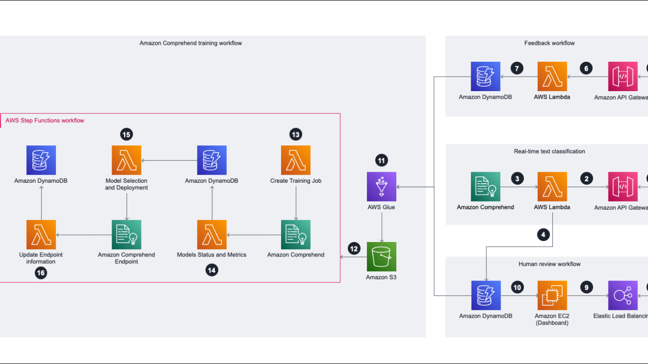
The following diagram illustrates the solution architecture covering real-time inference, feedback workflow, and human review workflow, and how those components contribute to the Amazon Comprehend training workflow.

In the following sections, we walk you through each step in the workflow.

Real-time text classification

To use Amazon Comprehend custom classification in real time, you need to deploy an API as the entry point and call an Amazon Comprehend model to conduct real-time text classification. The steps are as follows:

1. The client side calls Amazon API Gateway as the entry point to provide a client message as input.
2. API Gateway passes the request to AWS Lambda and calls the API from Amazon DynamoDB and Amazon Comprehend in Steps 3 and 4.
3. Lambda checks the current version of the Amazon Comprehend endpoint that stores data in DynamoDB, and calls an Amazon Comprehend endpoint to get real-time inference.
4. Lambda, with a built-in rule, checks the score to determine whether it’s under the threshold or not. It then stores that data in DynamoDB and waits for human approval to confirm the evaluation result.

Feedback workflow

When the endpoint returns the classification result to the client side, the application prompts the end-user with a hint to get their feedback, and stores the data in the database for the next round (the training workflow). The steps for the feedback workflow are as follows:

1. The client side sends the user feedback by calling API Gateway.
2. API Gateway bypasses the request to Lambda. Lambda checks the format and stores it in DynamoDB.
3. The user feedback from Lambda is stored in DynamoDB and will be used for the next training process.

Human review workflow

The human review process helps us clarify data with a confidence score below the threshold. This data is valuable for improving the Amazon Comprehend model, and is added to the next iteration of retraining. We used Elastic Load Balancing as the entry point to conduct this process because the Pro360 system is built on Amazon Elastic Complute Cloud (Amazon EC2). The steps for this workflow are as follows:

1. We use an existing API on the Elastic Load Balancer as the entry point.
2. We use Amazon EC2 as the compute resource to build a front-end dashboard for the reviewer to tag the input data with lower confidence scores.
3. After the reviewer identifies the objection from the input data, we store the result in a DynamoDB table.

Amazon Comprehend training workflow

To start the training the Amazon Comprehend model, we need to prepare the training data. The following steps show you how to train the model:

1. We use AWS Glue to conduct extract, transform, and load (ETL) jobs and merge the data from two different DynamoDB tables and store it in Amazon Simple Storage Service (Amazon S3).
2. When the Amazon S3 training data is ready, we can trigger AWS Step Functions as the orchestration tool to run the training job, and we pass the S3 path into the Step Functions state machine.
3. We invoke a Lambda function to validate that the training data path exists, and then trigger an Amazon Comprehend training job.
4. After the training job starts, we use another Lambda function to check the training job status. If the training job is complete, we get the model metric and store it in DynamoDB for further evaluation.
5. We check the performance of the current model with a Lambda model selection function. If the current version’s performance is better than the original one, we deploy it to the Amazon Comprehend endpoint.
6. Then we invoke another Lambda function to check the endpoint status. The function updates information in DynamoDB for real-time text classification when the endpoint is ready.

Summary and next steps

In this post, we showed how Amazon Comprehend enables Pro360 to build an AI-powered application without ML expert practitioners, which is able to increase the accuracy of customer objection detection. Pro360 was able to build a custom-purposed NLP model in just 1.5 months, and now is able to identify 90% of customer polite rejections and detect customer intent with 99.2% overall accuracy. This solution not only enhances the customer experience, increasing 28.5% retention rate growth, but also improves financial outcomes, decreasing the operation cost by 8% and reducing the workload for customer service agents.

However, identifying customer objections is just the first step in improving the customer experience. By continuing to iterate on the customer experience and accelerate revenue growth, the next step is to identify the reasons for customer objections, such as lack of interest, timing issues, or influence from others, and to generate the appropriate response to increase the sales conversion rate.

To use Amazon Comprehend to build custom text classification models, you can access the service through the AWS Management Console. To learn more about how to use Amazon Comprehend, check out Amazon Comprehend developer resources.

About the Authors

Ray Wang is a Solutions Architect at AWS. With 8 years of experience in the IT industry, Ray is dedicated to building modern solutions on the cloud, especially in NoSQL, big data, and machine learning. As a hungry go-getter, he passed all 12 AWS certificates to make his technical field not only deep but wide. He loves to read and watch sci-fi movies in his spare time.

Josie Cheng is a HKT AI/ML Go-To-Market at AWS. Her current focus is on business transformation in retail and CPG through data and ML to fuel tremendous enterprise growth. Before joining AWS, Josie worked for Amazon Retail and other China and US internet companies as a Growth Product Manager.

Shanna Chang is a Solutions Architect at AWS. She focuses on observability in modern architectures and cloud-native monitoring solutions. Before joining AWS, she was a software engineer. In her spare time, she enjoys hiking and watching movies.

Wrick Talukdar is a Senior Architect with the Amazon Comprehend Service team. He works with AWS customers to help them adopt machine learning on a large scale. Outside of work, he enjoys reading and photography.

Read More