Generative AI raises new challenges in defining, measuring, and mitigating concerns about fairness, toxicity, and intellectual property, among other things. But work has started on the solutions.Read More
Implement backup and recovery using an event-driven serverless architecture with Amazon SageMaker Studio
Amazon SageMaker Studio is the first fully integrated development environment (IDE) for ML. It provides a single, web-based visual interface where you can perform all machine learning (ML) development steps required to build, train, tune, debug, deploy, and monitor models. It gives data scientists all the tools you need to take ML models from experimentation to production without leaving the IDE. Moreover, as of November 2022, Studio supports shared spaces to accelerate real-time collaboration and multiple Amazon SageMaker domains in a single AWS Region for each account.
There are two prevailing use cases for Studio domain backup and recovery. The first use case involves a customer business unit and project wanting a functionality to replicate data scientists’ artifacts and data files to any target domains and profiles at will. The second use case involves the replication only when the domain and profile are deleted due to conditions such as the change from a customer-managed key to an AWS-managed key or a change of onboarding from AWS Identity and Access Management (IAM) authentication (see Onboard to Amazon SageMaker Domain Using IAM) to AWS IAM Identity Center (see Onboard to Amazon SageMaker Domain Using IAM Identity Center).
This post mainly covers the second use case by presenting how to back up and recover users’ work when the user and space profiles are deleted and recreated, but we also provide the Python script to support the first use case.
When the user and space profiles are recreated in the existing Studio domain, a new ID of the profile directory will be created within the Studio Amazon Elastic File System (Amazon EFS) volume. As a result, the Studio users could lose access to the model artifacts and data files stored in their previous profile directory if they are deleted. Additionally, Studio domains don’t currently support mounting custom or additional EFS volumes. We recommend keeping the previous Studio EFS volume as a backup using RetentionPolicy in Studio.
Therefore, a proper recovery solution needs to be implemented to access the data from the previous directory in case of profile deletion or to recover files from a detached volume in case of domain deletion. Data scientists can minimize the potential impacts of deleting the domain and profiles if they frequently commit their code to the repository and utilize external storage for data access. However, having the capability to back up and recover the data scientist’s workspace is another layer to ensure their continuity of work, which may increase their productivity. Moreover, if you have tens and hundreds of Studio users, consider how to automate the recovery process to avoid mistakes and save costs and time. To solve this problem, we provide a solution to supplement Studio domain recovery.
This post explains the backup and recovery module and one approach to automate the process using an event-driven architecture. First, we demonstrate how to perform backup and recovery if you create a new Studio domain, user, and space profiles using AWS CloudFormation templates. Next, we explain the required steps to test our recovery solution using the existing domain and profiles without using our CloudFormation templates (you can use your own templates). Although this post focuses on a single domain setting, our solution works for multiple Studio domains as well. Finally, we have automated the provisioning of all resources using the AWS Serverless Application Model (AWS SAM), an open-source framework for building serverless applications.
Solution overview
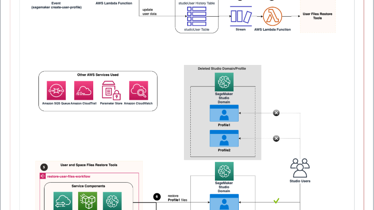
The following diagram illustrates the high-level workflow of Studio domain backup and recovery with an event-driven architecture.

The event-driven app includes the following steps:
- An Amazon CloudWatch events rule uses AWS CloudTrail to track
CreateUserProfileandCreateSpaceAPI calls, trigger the rule, and invoke the AWS Lambda function. - The function updates the user table and appends items in the history table in Amazon DynamoDB. In addition, the database layer keeps track of the domain and profile name and file system mapping.
The following image shows the DynamoDB tables structure. The partition key and sort key in the studioUser table consist of the profile and domain name. The replication column holds the replication flag with true as the default value. In addition, bytes_written, bytes_file_transferred, total_duration_ms, and replication_status fields are populated when the replication completes successfully.

The database layer can be replaced by other services, such as Amazon Relational Database Service (Amazon RDS) or Amazon Simple Storage Service (Amazon S3). However, we chose DynamoDB because of the Amazon DynamoDB Streams feature.
- DynamoDB Streams is enabled on the user table, and the Lambda function is set as a trigger and synchronously invoked when new stream records are available.
- Another Lambda function triggers the process to restore the files using the user and space files restore tools.
The backup and recovery workflow includes the following steps:
- The backup and recovery workflow consists of AWS Step Functions, integrated with other AWS services, including AWS DataSync, to orchestrate the recovery of the user and space files from the previous directory to a new directory between the same Studio domain EFS volume (profile recreation) or a new domain EFS volume (domain recreation). With the Step Functions Workflow Studio, the workflow can be implemented with no code (such as in this case) or low code for a more customized solution. The Step Functions state machine is invoked when the event-driven app detects the profile creation event. For each profile, the Step Functions state machine runs the DataSync task to copy all files from their previous directories to the new directory.
The following image is the actual graph of the Step Functions state machine. Note that the ListApp* step ensures the profile directories are populated in the Studio EFS volume before proceeding. Also, we implemented retry with exponential backoff to handle API throttle for DataSync CreateLocationEfs and CreateTask API calls.

- When the users open their Studio, all the files from the respective directories from the previous directory will be available to continue their work. The DataSync job replicating one gigabyte of data from our experiment took approximately 1 minute.
The following are services that will be used as part of the solution:
- AWS CloudFormation
- AWS CloudTrail
- Amazon CloudWatch
- AWS DataSync
- Amazon DynamoDB
- AWS Identity and Access Management (IAM)
- AWS Lambda
- Amazon SageMaker Studio
- Amazon Simple Queue Service (Amazon SQS)
- AWS Step Functions
- AWS Systems Manager
Prerequisites
To implement this solution, you must have the following prerequisites:
- An AWS account if you don’t already have one. The IAM user that you use must have sufficient permissions to make the necessary AWS service calls and manage AWS resources.
- The AWS SAM CLI installed and configured.
- Your AWS credentials set up.
- Git installed.
- Python 3.9.
- A Studio profile and domain name combination that is unique across all Studio domains within a Region and account.
- You need to use the existing Amazon VPC and S3 bucket to follow the deployment step.
- Also, be aware of the service quota for the maximum number of DataSync tasks per account per Region (default is 100). You can request a quota increase to meet the number of replication tasks for your use case.
Refer to the AWS Regional Services List for service availability based on Region. Additionally, review Amazon SageMaker endpoints and quotas.
Set up a Studio profile recovery infrastructure
The following diagram shows the logical steps for a SageMaker administrator to set up the Studio user and space recovery infrastructure, which a single command can complete with our automated solution.

To set up the environment, clone the GitHub repo in the terminal:
The following code shows the deployment script usage:
To create a new Amazon SageMaker domain, run the following command. You need to specify which Amazon VPC and subnet you want to use. We use VPC only mode for the Studio deployment. If you don’t have any preference, you can use the default VPC and subnet. Also, specify any stack name, AWS Region, and S3 bucket name for AWS SAM to deploy the Lambda function:
If you want to use an existing Studio domain, run the following command. Option -d yes will skip creating a new Studio domain:
For the existing domains, the SageMaker administrator must also update the source and target Studio EFS security groups to allow connection to the user and space file restore tool. For example, to run the following command, you need to specify HomeEfsFileSystemId, the EFS file system ID, and SecurityGroupId used by the user and space file restore tool (we discuss this in more detail later in the post):
User and space recovery logical flow
The following diagram shows the logical user and space recovery flow diagram for a SageMaker administrator to understand how the solution works, and no additional setup is required. If the profile (user or space) and domain are accidentally deleted, the EFS volume is detached but not deleted. A possible scenario is that we may want to revert the deletion by recreating a new domain and profiles. If the same profiles are being onboarded again, they may wish to access the files from their respective workspace in the detached volume. The recovery process is almost entirely automated; the only action required by the SageMaker administrator is to recreate the Studio domain and profiles using the same CloudFormation template. The rest of the steps are automated.

Optionally, if the SageMaker admin wants control over replication, run the following command to turn off replication for specific domains and profiles. This script updates the replication field given the domain and profile name in the table. Note that you need to run the script for the same user each time they get recreated.
The following optional step provides the solution for the first use case to allow replication to take place between the specified source file system to any target domain and profile name. If the SageMaker admin wants to replicate particular profile data to a different domain and a profile that doesn’t exist yet, run the following command. The script inserts the new domain and profile name with the specified source file system information. The subsequent profile creation will trigger the replication task. Note that you need to run add-security-group.py from the previous step to allow connection to the file restore tool.
In the following sections, we test two scenarios to confirm that the solution works as expected.
Create a new Studio domain
Our first test scenario assumes you are starting from scratch and want to create a new Studio domain and profiles in your environment using our templates. Then we deploy the Studio domain, user and space, backup and recovery workflow, and event app. The purpose of the first scenario is to confirm that the profile file is recovered in the new home directory automatically when the profile is deleted and recreated within the same Studio domain.
Complete the following steps:
- To deploy the application, run the following command:
- On the AWS CloudFormation console, ensure the following stacks are in
CREATE_COMPLETEstatus:<stack_name>-DemoBootstrap-*<stack_name>-StepFunction-*<stack_name>-EventApp-*<stack_name>-StudioDomain-*<stack_name>-StudioUser1-*<stack_name>-StudioSpace-*

If the deployment failed in any stacks, check the error and resolve the issues. Then, proceed to the next step only if the problems are resolved.
- On the DynamoDB console, choose Tables in the navigation pane and confirm that the
studioUserandstudioUserHistorytables are created. - Select
studioUserand choose Explore table items to confirm that items foruser1andspace1are populated in the table. - On the SageMaker console, choose Domains in the navigation pane.
- Choose
demo-myapp-dev-studio-domain. - On the User profiles tab, select
user1and choose Launch, and choose Studio to open the Studio for the user.
Note that Studio may take 10-15 minutes to load for the first time.
- On the File menu, choose Terminal to launch a new terminal within Studio.
- Run the following command in the terminal to create a file for testing:
- Repeat these steps for
space1(choose Spaces in Step 7). Feel free to create a file of your choice. - Delete the Studio user
user1andspace1by removing the nested stacks<stack_name>and-StudioUser1-*<stack_name>-StudioSpace-*from the parent. Delete the stacks by commenting out the following code blocks from the AWS SAM template file,template.yaml. Make sure to save the file after the edit:
- Run the following command to deploy the stack with this change:
- Recreate the Studio profiles by adding back the stack back to the parent. Uncomment the code block from the previous step, save the file, and run the same command:
After a successful deployment, you can check the results.
- On the AWS CloudFormation console, choose the stack
<stack_name>-StepFunction-* - In the stack, choose the value for Physical ID of
StepFunctionin the Resources section. - Choose the most recent run and confirm its status in Graph view.
It should look like the following screenshot for the user profile replication. You can also check the other run to ensure the same for the space profile.

- If you completed Steps 5–10, open the Studio domain for
user1and confirm that theuser1.txtfile is copied to the newly created directory.
It should not be visible in space1 directory, keeping the same file ownership.
- Repeat this step for
space1. - On the DataSync console, choose the most recent task ID.
- Choose History and the most recent run ID.
This is another way to inspect the configurations and the run status of the DataSync task. As an example, the following screenshot shows the task result for user1 directory replication.

We only covered profile recreation in this scenario. However, our solution works in the same way for Studio domain recreation, and it can be tested by deleting and recreating the domain.
Use an existing Studio domain
Our second test scenario assumes you want to use the existing SageMaker domain and profiles in the environment. Therefore, we only deploy the backup and recovery workflow and the event app. Again, you can use your own Studio CloudFormation template or create them through the AWS CloudFormation console to follow along. Because we’re using the existing Studio domain, the solution will list the current user and space for all domains within the Region, which we call seeding.
Complete the following steps:
- To deploy the application, run the following command:
- On the AWS CloudFormation console, ensure the following stacks are in
CREATE_COMPLETEstatus:<stack_name>-DemoBootstrap-*<stack_name>-StepFunction-*<stack_name>-EventApp-*
If the deployment failed in any stacks, check the error and resolve the issues. Then, proceed to the next step only if the problems are resolved.
- Verify the initial data seed has completed.
- On the DynamoDB console, choose Tables in the navigation pane and confirm that the
studioUserandstudioUserHistorytables are created. - Choose
studioUserand choose Explore table items to confirm that items for the existing Studio domain are populated in the table.
Proceed to the next step only if the seed has completed successfully. If the tables aren’t populated, check the CloudWatch logs of the corresponding Lambda function. On the AWS CloudFormation console, choose the stack <stack_name>, and choose the physical ID of -EventApp-*DDBSeedLambda in the Resources section. Under Monitor, choose View CloudWatch Logs and check the logs for the most recent run to troubleshoot.
- To update the EFS security group, first get the
SecurityGroupId. We use the security group created by the CloudFormation template, which allows all traffic in the outbound connection. Run the following command:
- Get the
HomeEfsFileSystemId, which is the ID of the Studio home EFS volume. Run the following command: - Finally, update the EFS security group by allowing inbounds from the security group shared with the DataSync task using port 2049. Run the following command:
- Delete and recreate the Studio profiles of your choice using the same profile name.
- Confirm the run status of the Step Functions state machine and recovery of the Studio profile directory by following the steps from the first scenario.
You can also test the Step Functions workflow manually with your choice of source and target inputs for replication (more details found in README.md in the GitHub repository).
Clean up
Run the following commands to clean up your resources:
Manually delete the SageMakerSecurityGroup after 20 minutes or so. Deletion of the Elastic Network Interface (ENI) can make the stack show as DELETE_IN_PROGRESS for some time, so we intentionally set the security group to be retained. Also, you need to disassociate that security group from the security group managed by SageMaker before you can delete it.
Conclusion
Studio is a powerful IDE that allows data scientists to quickly develop, train, test, and deploy models. This post discusses how to back up and recover the files stored in a data scientist’s home and shared space directory. We also demonstrated how an event-driven architecture can help automate the recovery process.
Our solution can help improve the resiliency of data scientists’ artifacts within Studio, leading to operational efficiency on the AWS Cloud. Also, the solution is modular, so you can use the necessary components and update them for your usage. For instance, the enhancement to this solution might be a cross-account replication. We hope that what we demonstrated in the post will be a helpful resource to support those ideas.
To get started with Studio, check out Amazon SageMaker for Data Scientists. Please send us feedback on the AWS forum for SageMaker or through your AWS support contacts. You can find other Studio examples in our GitHub repository.
About the Authors
 Kenny Sato is a Machine Learning Engineer at AWS, guiding customers in architecting and implementing machine learning solutions. He received his master’s in Computer Engineering from Virginia Tech and is pursuing a PhD in Computer Science. In his spare time, you can find him in his backyard or out somewhere playing with his lovely daughters.
 Gautam Nambiar is a DevOps Consultant with AWS. He is particularly interested in architecting and building automated solutions, MLOps pipelines, and creating reusable and secure DevOps best practice patterns. In his spare time, he likes playing and watching soccer.
Optimized PyTorch 2.0 inference with AWS Graviton processors
New generations of CPUs offer a significant performance improvement in machine learning (ML) inference due to specialized built-in instructions. Combined with their flexibility, high speed of development, and low operating cost, these general-purpose processors offer an alternative to other existing hardware solutions.
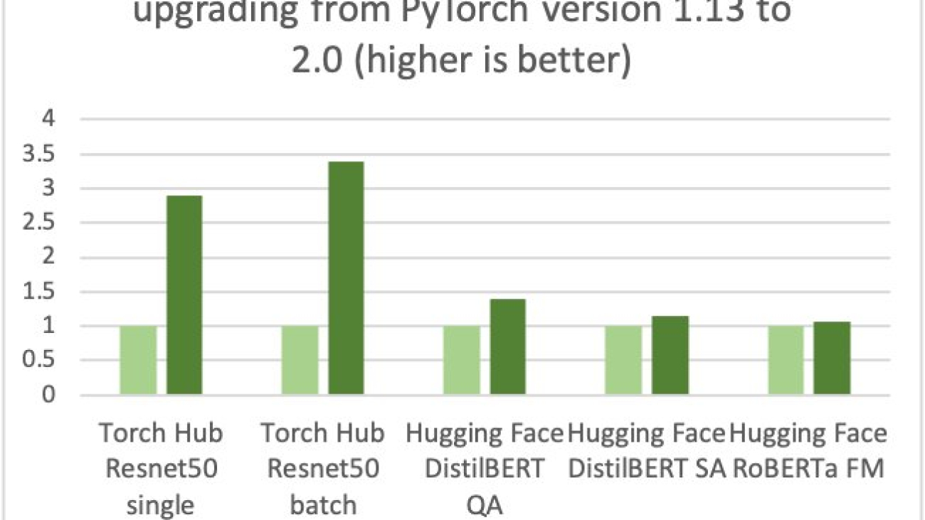
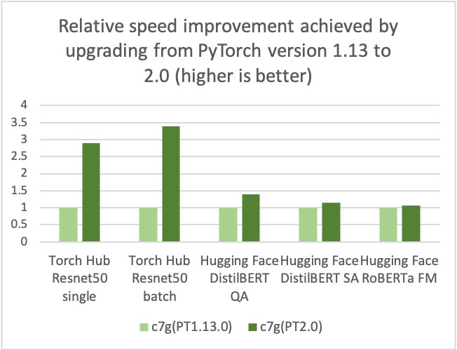
AWS, Arm, Meta and others helped optimize the performance of PyTorch 2.0 inference for Arm-based processors. As a result, we are delighted to announce that AWS Graviton-based instance inference performance for PyTorch 2.0 is up to 3.5 times the speed for Resnet50 compared to the previous PyTorch release (see the following graph), and up to 1.4 times the speed for BERT, making Graviton-based instances the fastest compute optimized instances on AWS for these models.
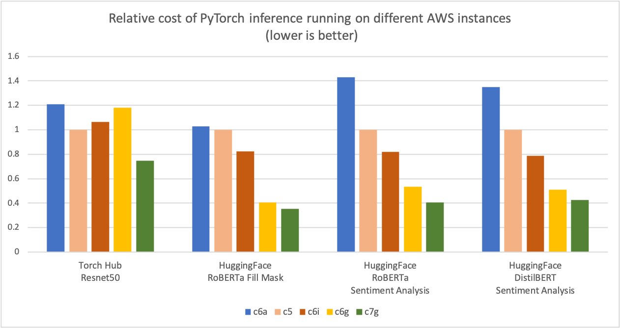
AWS measured up to 50% cost savings for PyTorch inference with AWS Graviton3-based Amazon Elastic Cloud Compute C7g instances across Torch Hub Resnet50, and multiple Hugging Face models relative to comparable EC2 instances, as shown in the following figure.
Additionally, the latency of inference is also reduced, as shown in the following figure.

We have seen a similar trend in the price-performance advantage for other workloads on Graviton, for example video encoding with FFmpeg.
Optimization details
The optimizations focused on three key areas:
- GEMM kernels – PyTorch supports Arm Compute Library (ACL) GEMM kernels via the OneDNN backend (previously called MKL-DNN) for Arm-based processors. The ACL library provides Neon and SVE optimized GEMM kernels for both fp32 and bfloat16 formats. These kernels improve the SIMD hardware utilization and reduce the end-to-end inference latencies.
- bfloat16 support – The bfloat16 support in Graviton3 allows for efficient deployment of models trained using bfloat16, fp32, and AMP (Automatic Mixed Precision). The standard fp32 models use bfloat16 kernels via OneDNN fast math mode, without model quantization, providing up to two times faster performance compared to the existing fp32 model inference without bfloat16 fast math support.
- Primitive caching – We also implemented primitive caching for conv, matmul, and inner product operators to avoid redundant GEMM kernel initialization and tensor allocation overhead.
How to take advantage of the optimizations
The simplest way to get started is by using the AWS Deep Learning Containers (DLCs) on Amazon Elastic Compute Cloud (Amazon EC2) C7g instances or Amazon SageMaker. DLCs are available on Amazon Elastic Container Registry (Amazon ECR) for AWS Graviton or x86. For more details on SageMaker, refer to Run machine learning inference workloads on AWS Graviton-based instances with Amazon SageMaker and Amazon SageMaker adds eight new Graviton-based instances for model deployment.
Use AWS DLCs
To use AWS DLCs, use the following code:
If you prefer to install PyTorch via pip, install the PyTorch 2.0 wheel from the official repo. In this case, you will have to set two environment variables as explained in the code below before launching PyTorch to activate the Graviton optimization.
Use the Python wheel
To use the Python wheel, refer to the following code:
Run inference
You can use PyTorch TorchBench to measure the CPU inference performance improvements, or to compare different instance types:
Benchmarking
You can use the Amazon SageMaker Inference Recommender utility to automate performance benchmarking across different instances. With Inference Recommender, you can find the real-time inference endpoint that delivers the best performance at the lowest cost for a given ML model. We collected the preceding data using the Inference Recommender notebooks by deploying the models on production endpoints. For more details on Inference Recommender, refer to the GitHub repo. We benchmarked the following models for this post: ResNet50 image classification, DistilBERT sentiment analysis, RoBERTa fill mask, and RoBERTa sentiment analysis.
Conclusion
AWS measured up to 50% cost savings for PyTorch inference with AWS Graviton3-based Amazon Elastic Cloud Compute C7g instances across Torch Hub Resnet50, and multiple Hugging Face models relative to comparable EC2 instances. These instances are available on SageMaker and Amazon EC2. The AWS Graviton Technical Guide provides the list of optimized libraries and best practices that will help you achieve cost benefits with Graviton instances across different workloads.
If you find use cases where similar performance gains aren’t observed on AWS Graviton, please open an issue on the AWS Graviton Technical Guide to let us know about it. We will continue to add more performance improvements to make Graviton the most cost-effective and efficient general-purpose processor for inference using PyTorch.
About the author
 Sunita Nadampalli is a Software Development Manager at AWS. She leads Graviton software performance optimizations for machine leaning, HPC, and multimedia workloads. She is passionate about open-source development and delivering cost-effective software solutions with Arm SoCs.
How Vericast optimized feature engineering using Amazon SageMaker Processing
This post is co-written by Jyoti Sharma and Sharmo Sarkar from Vericast.
For any machine learning (ML) problem, the data scientist begins by working with data. This includes gathering, exploring, and understanding the business and technical aspects of the data, along with evaluation of any manipulations that may be needed for the model building process. One aspect of this data preparation is feature engineering.
Feature engineering refers to the process where relevant variables are identified, selected, and manipulated to transform the raw data into more useful and usable forms for use with the ML algorithm used to train a model and perform inference against it. The goal of this process is to increase the performance of the algorithm and resulting predictive model. The feature engineering process entails several stages, including feature creation, data transformation, feature extraction, and feature selection.
Building a platform for generalized feature engineering is a common task for customers needing to produce many ML models with differing datasets. This kind of platform includes the creation of a programmatically driven process to produce finalized, feature engineered data ready for model training with little human intervention. However, generalizing feature engineering is challenging. Each business problem is different, each dataset is different, data volumes vary wildly from client to client, and data quality and often cardinality of a certain column (in the case of structured data) might play a significant role in the complexity of the feature engineering process. Furthermore, the dynamic nature of a customer’s data can also result in a large variance of the processing time and resources required to optimally complete the feature engineering.
AWS customer Vericast is a marketing solutions company that makes data-driven decisions to boost marketing ROIs for its clients. Vericast’s internal cloud-based Machine Learning Platform, built around the CRISP-ML(Q) process, uses various AWS services, including Amazon SageMaker, Amazon SageMaker Processing, AWS Lambda, and AWS Step Functions, to produce the best possible models that are tailored to the specific client’s data. This platform aims at capturing the repeatability of the steps that go into building various ML workflows and bundling them into standard generalizable workflow modules within the platform.
In this post, we share how Vericast optimized feature engineering using SageMaker Processing.
Solution overview
Vericast’s Machine Learning Platform aids in the quicker deployment of new business models based on existing workflows or quicker activation of existing models for new clients. For example, a model predicting direct mail propensity is quite different from a model predicting discount coupon sensitivity of the customers of a Vericast client. They solve different business problems and therefore have different usage scenarios in a marketing campaign design. But from an ML standpoint, both can be construed as binary classification models, and therefore could share many common steps from an ML workflow perspective, including model tuning and training, evaluation, interpretability, deployment, and inference.
Because these models are binary classification problems (in ML terms), we are separating the customers of a company into two classes (binary): those that would respond positively to the campaign and those that would not. Furthermore, these examples are considered an imbalanced classification because the data used to train the model wouldn’t contain an equal number of customers who would and would not respond favorably.
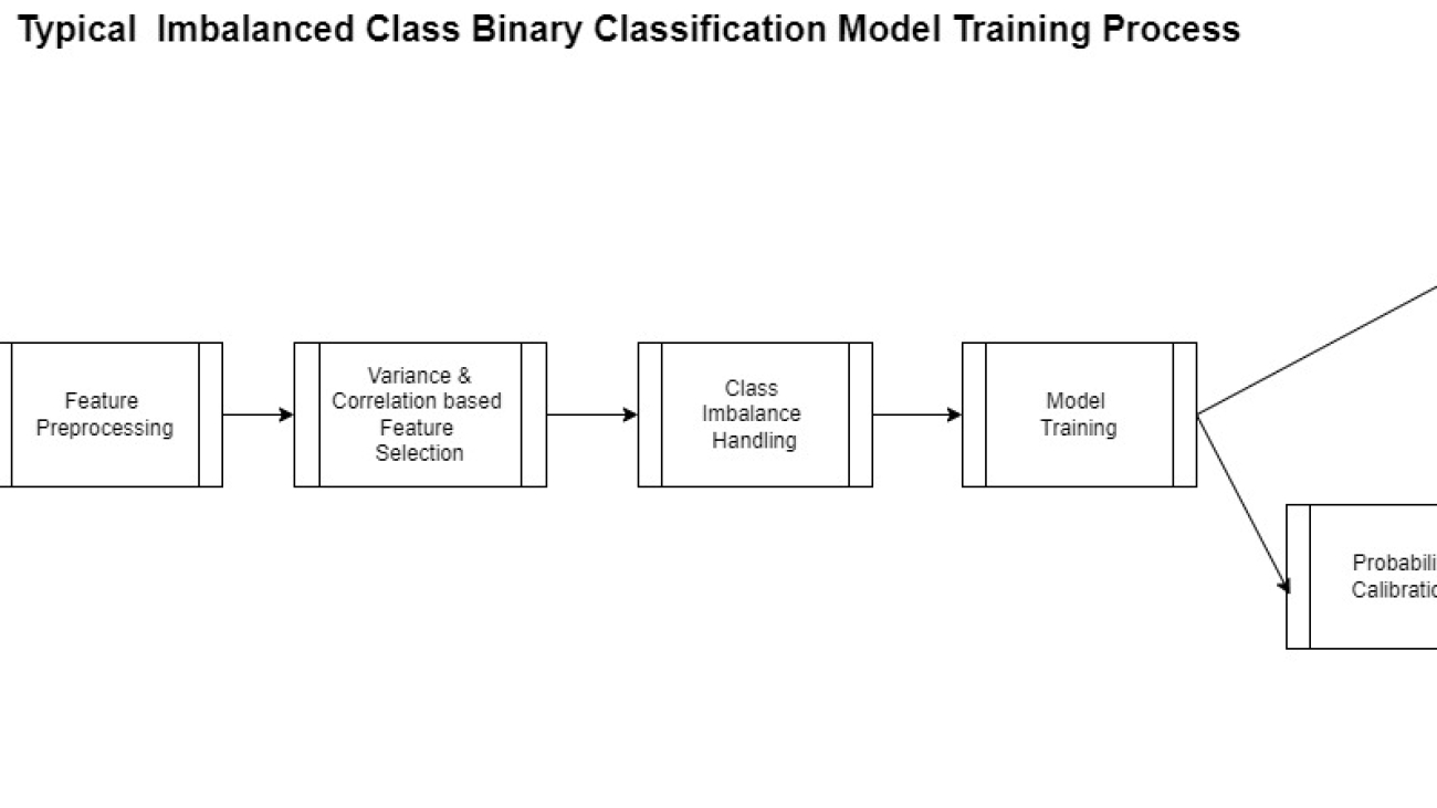
The actual creation of a model such as this follows the generalized pattern shown in the following diagram.
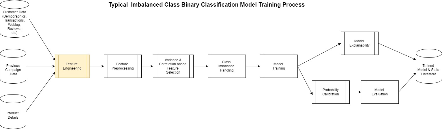
Most of this process is the same for any binary classification except for the feature engineering step. This is perhaps the most complicated yet at times overlooked step in the process. ML models are largely dependent on the features used to create it.
Vericast’s cloud-native Machine Learning Platform aims to generalize and automate the feature engineering steps for various ML workflows and optimize their performance on a cost vs. time metric by using the following features:
- The platform’s feature engineering library – This consists of an ever-evolving set of transformations that have been tested to yield high-quality generalizable features based on specific client concepts (for example, customer demographics, product details, transaction details, and so on).
- Intelligent resource optimizers – The platform uses AWS’s on-demand infrastructure capability to spin up the most optimal type of processing resources for the particular feature engineering job based on the expected complexity of the step and the amount of data it needs to churn through.
- Dynamic scaling of feature engineering jobs – A combination of various AWS services is used for this, but most notably SageMaker Processing. This ensures that the platform produces high-quality features in a cost-efficient and timely manner.
This post is focused around the third point in this list and shows how to achieve dynamic scaling of SageMaker Processing jobs to achieve a more managed, performant, and cost-effective data processing framework for large data volumes.
SageMaker Processing enables workloads that run steps for data preprocessing or postprocessing, feature engineering, data validation, and model evaluation on SageMaker. It also provides a managed environment and removes the complexity of undifferentiated heavy lifting required to set up and maintain the infrastructure needed to run the workloads. Furthermore, SageMaker Processing provides an API interface for running, monitoring, and evaluating the workload.
Running SageMaker Processing jobs takes place fully within a managed SageMaker cluster, with individual jobs placed into instance containers at run time. The managed cluster, instances, and containers report metrics to Amazon CloudWatch, including usage of GPU, CPU, memory, GPU memory, disk metrics, and event logging.
These features provide benefits to Vericast data engineers and scientists by assisting in the development of generalized preprocessing workflows and abstracting the difficulty of maintaining generated environments in which to run them. Technical problems can arise, however, given the dynamic nature of the data and its varied features that can be fed into such a general solution. The system must make an educated initial guess as to the size of the cluster and instances that compose it. This guess needs to evaluate criteria of the data and infer the CPU, memory, and disk requirements. This guess may be wholly appropriate and perform adequately for the job, but in other cases it may not. For a given dataset and preprocessing job, the CPU may be undersized, resulting in maxed out processing performance and lengthy times to complete. Worse yet, memory could become an issue, resulting in either poor performance or out of memory events causing the entire job to fail.
With these technical hurdles in mind, Vericast set out to create a solution. They needed to remain general in nature and fit into the larger picture of the preprocessing workflow being flexible in the steps involved. It was also important to solve for both the potential need to scale up the environment in cases where performance was compromised and to gracefully recover from such an event or when a job finished prematurely for any reason.
The solution built by Vericast to solve this issue uses several AWS services working together to reach their business objectives. It was designed to restart and scale up the SageMaker Processing cluster based on performance metrics observed using Lambda functions monitoring the jobs. To not lose work when a scaling event takes place or to recover from a job unexpectedly stopping, a checkpoint-based service was put in place that uses Amazon DynamoDB and stores the partially processed data in Amazon Simple Storage Service (Amazon S3) buckets as steps complete. The final outcome is an auto scaling, robust, and dynamically monitored solution.
The following diagram shows a high-level overview of how the system works.

In the following sections, we discuss the solution components in more detail.
Initializing the solution
The system assumes that a separate process initiates the solution. Conversely, this design is not designed to work alone because it won’t yield any artifacts or output, but rather acts as a sidecar implementation to one of the systems that use SageMaker Processing jobs. In Vericast’s case, the solution is initiated by way of a call from a Step Functions step started in another module of the larger system.
Once the solution initiated and a first run is triggered, a base standard configuration is read from a DynamoDB table. This configuration is used to set parameters for the SageMaker Processing job and has the initial assumptions of infrastructure needs. The SageMaker Processing job is now started.
Monitoring metadata and output
When the job starts, a Lambda function writes the job processing metadata (the current job configuration and other log information) into the DynamoDB log table. This metadata and log information maintains a history of the job, its initial and ongoing configuration, and other important data.
At certain points, as steps complete in the job, checkpoint data is added to the DynamoDB log table. Processed output data is moved to Amazon S3 for quick recovery if needed.
This Lambda function also sets up an Amazon EventBridge rule that monitors the running job for its state. Specifically, this rule is watching the job to observe if the job status changes to stopping or is in a stopped state. This EventBridge rule plays an important part in restarting a job if there is a failure or a planned auto scaling event occurs.
Monitoring CloudWatch metrics
The Lambda function also sets a CloudWatch alarm based on a metric math expression on the processing job, which monitors the metrics of all the instances for CPU utilization, memory utilization, and disk utilization. This type of alarm (metric) uses CloudWatch alarm thresholds. The alarm generates events based on the value of the metric or expression relative to the thresholds over a number of time periods.
In Vericast’s use case, the threshold expression is designed to consider the driver and the executor instances as separate, with metrics monitored individually for each. By having them separate, Vericast knows which is causing the alarm. This is important to decide how to scale accordingly:
- If the executor metrics are passing the threshold, it’s good to scale horizontally
- If the driver metrics cross the threshold, scaling horizontally will probably not help, so we must scale vertically
Alarm metrics expression
Vericast can access the following metrics in its evaluation for scaling and failure:
- CPUUtilization – The sum of each individual CPU core’s utilization
- MemoryUtilization – The percentage of memory that is used by the containers on an instance
- DiskUtilization – The percentage of disk space used by the containers on an instance
- GPUUtilization – The percentage of GPU units that are used by the containers on an instance
- GPUMemoryUtilization – The percentage of GPU memory used by the containers on an instance
As of this writing, Vericast only considers CPUUtilization, MemoryUtilization, and DiskUtilization. In the future, they intend to consider GPUUtilization and GPUMemoryUtilization as well.
The following code is an example of a CloudWatch alarm based on a metric math expression for Vericast auto scaling:
This expression illustrates that the CloudWatch alarm is considering DriverMemoryUtilization (memoryDriver), CPUUtilization (cpuDriver), DiskUtilization (diskDriver), ExecutorMemoryUtilization (memoryExec), CPUUtilization (cpuExec), and DiskUtilization (diskExec) as monitoring metrics. The number 80 in the preceding expression stands for the threshold value.
Here, IF((cpuDriver) > 80, 1, 0 implies that if the driver CPU utilization goes beyond 80%, 1 is assigned as the threshold else 0. IF(AVG(METRICS("memoryExec")) > 80, 1, 0 implies that all the metrics with string memoryExec in it are considered and an average is calculated on that. If that average memory utilization percentage goes beyond 80, 1 is assigned as the threshold else 0.
The logical operator OR is used in the expression to unify all the utilizations in the expression—if any of the utilizations reach its threshold, trigger the alarm.
For more information on using CloudWatch metric alarms based on metric math expressions, refer to Creating a CloudWatch alarm based on a metric math expression.
CloudWatch alarm limitations
CloudWatch limits the number of metrics per alarm to 10. This can cause limitations if you need to consider more metrics than this.
To overcome this limitation, Vericast has set alarms based on the overall cluster size. One alarm is created per three instances (for three instances, there will be one alarm because that would add up to nine metrics). Assuming the driver instance is to be considered separately, another separate alarm is created for the driver instance. Therefore, the total number of alarms that are created are roughly equivalent to one third the number of executor nodes and an additional one for the driver instance. In each case, the number of metrics per alarm is under the 10 metric limitation.
What happens when in an alarm state
If a predetermined threshold is met, the alarm goes to an alarm state, which uses Amazon Simple Notification Service (Amazon SNS) to send out notifications. In this case, it sends out an email notification to all subscribers with the details about the alarm in the message.
Amazon SNS is also used as a trigger to a Lambda function that stops the currently running SageMaker Processing job because we know that the job will probably fail. This function also records logs to the log table related to the event.
The EventBridge rule set up at job start will notice that the job has gone into a stopping state a few seconds later. This rule then reruns the first Lambda function to restart the job.
The dynamic scaling process
The first Lambda function after running two or more times will know that a previous job had already started and now has stopped. The function will go through a similar process of getting the base configuration from the original job in the log DynamoDB table and will also retrieve updated configuration from the internal table. This updated configuration is a resources delta configuration that is set based on the scaling type. The scaling type is determined from the alarm metadata as described earlier.
The original configuration plus the resources delta are used because a new configuration and a new SageMaker Processing job are started with the increased resources.
This process continues until the job completes successfully and can result in multiple restarts as needed, adding more resources each time.
Vericast’s outcome
This custom auto scaling solution has been instrumental in making Vericast’s Machine Learning Platform more robust and fault tolerant. The platform can now gracefully handle workloads of different data volumes with minimal human intervention.
Before implementing this solution, estimating the resource requirements for all the Spark-based modules in the pipeline was one of the biggest bottlenecks of the new client onboarding process. Workflows would fail if the client data volume increased, or the cost would be unjustifiable if the data volume decreased in production.
With this new module in place, workflow failures due to resource constraints have been reduced by almost 80%. The few remaining failures are mostly due to AWS account constraints and beyond the auto scale process. Vericast’s biggest win with this solution is the ease with which they can onboard new clients and workflows. Vericast expects to speed up the process by at least 60–70%, with data still to be gathered for a final number.
Though this is viewed as a success by Vericast, there is a cost that comes with it. Based on the nature of this module and the concept of dynamic scaling as a whole, the workflows tend to take around 30% longer (average case) than a workflow with a custom-tuned cluster for each module in the workflow. Vericast continues to optimize in this area, looking to improve the solution by incorporating heuristics-based resource initialization for each client module.
Sharmo Sarkar, Senior Manager, Machine Learning Platform at Vericast, says, “As we continue to expand our use of AWS and SageMaker, I wanted to take a moment to highlight the incredible work of our AWS Client Services Team, dedicated AWS Solutions Architects, and AWS Professional Services that we work with. Their deep understanding of AWS and SageMaker allowed us to design a solution that met all of our needs and provided us with the flexibility and scalability we required. We are so grateful to have such a talented and knowledgeable support team on our side.”
Conclusion
In this post, we shared how SageMaker and SageMaker Processing have enabled Vericast to build a managed, performant, and cost-effective data processing framework for large data volumes. By combining the power and flexibility of SageMaker Processing with other AWS services, they can easily monitor the generalized feature engineering process. They can automatically detect potential issues generated from lack of compute, memory, and other factors, and automatically implement vertical and horizontal scaling as needed.
SageMaker and its tools can help your team meet its ML goals as well. To learn more about SageMaker Processing and how it can assist in your data processing workloads, refer to Process Data. If you’re just getting started with ML and are looking for examples and guidance, Amazon SageMaker JumpStart can get you started. JumpStart is an ML hub from which you can access built-in algorithms with pre-trained foundation models to help you perform tasks such as article summarization and image generation and pre-built solutions to solve common use cases.
Finally, if this post helps you or inspires you to solve a problem, we would love to hear about it! Please share your comments and feedback.
About the Authors
 Anthony McClure is a Senior Partner Solutions Architect with the AWS SaaS Factory team. Anthony also has a strong interest in machine learning and artificial intelligence working with the AWS ML/AI Technical Field Community to assist customers in bringing their machine learning solutions to reality.
 Jyoti Sharma is a Data Science Engineer with the machine learning platform team at Vericast. She is passionate about all aspects of data science and focused on designing and implementing a highly scalable and distributed Machine Learning Platform.
 Sharmo Sarkar is a Senior Manager at Vericast. He leads the Cloud Machine Learning Platform and the Marketing Platform ML R&D Teams at Vericast. He has extensive experience in Big Data Analytics, Distributed Computing, and Natural Language Processing. Outside work, he enjoys motorcycling, hiking, and biking on mountain trails.
Amazon provides gift to 10 Penn PhD students for work on trustworthy AI
Projects are centered around themes of fairness, privacy, explainability, and interpretability.Read More

Try 4 new Arts and AI experiments
 Four new online interactive artworks from Google Arts & Culture Lab artists in residenceRead More
Announcing PyTorch Docathon 2023

We are excited to announce the first ever PyTorch Docathon! The Docathon is a hackathon-style event focused on improving the documentation by enlisting the help of the community. Documentation is a crucial aspect of any technology and by improving the documentation, we can make it easier for users to get started with PyTorch, help them understand how to use its features effectively, and ultimately accelerate research to production in the field of machine learning.
WHY PARTICIPATE
Low Barrier to Entry
Many open-source projects require extensive knowledge of the codebase and prior contributions to the project to participate in any sort of hackathon events. The Docathon, on the other hand, is designed for newcomers. We do expect familiarity with Python, basic knowledge of PyTorch, and ML. But don’t fret, there are some tasks that are related to website issues that won’t require even that.
Tangible Results
One of the best things about the Docathon is that you can see the results of your efforts in real time. Improving documentation can have a huge impact on a project’s usability and accessibility and you’ll be able to see those improvements firsthand. Plus having tangible results can be a great motivator to keep contributing.
Collaborative Environment
The Docathon is a collaborative event which means you’ll have the opportunity to work with other contributors and PyTorch maintainers on improving the documentation. This can be a great way to learn from others, share ideas, and build connections.
Learning Opportunities
Finally, even if you are not an expert in PyTorch, the Docathon can be a great learning experience. You’ll have the opportunity to explore the PyTorch modules and test some of the tutorials on your machine as well as in the CI.
EVENT DETAILS
- May 31: Kick-off
- May 31 – June 11: Submissions and Feedback
- June 12 – June 13: Final Reviews
- June 15: Winner Announcements
Details for the Docathon to be announced at the kick-off stream on May 31.
Please register to join this year’s event: RSVP
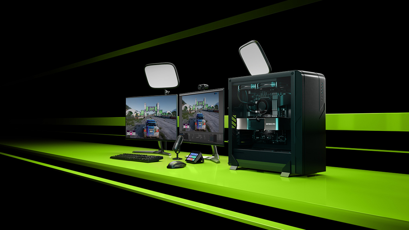
Picture Perfect: AV1 Streaming Dazzles on GeForce RTX 40 Series GPUs With OBS Studio 29.1 Launch and YouTube Support
AV1, the next-generation video codec, is expanding its reach with today’s release of OBS Studio 29.1. This latest software update adds support for AV1 streaming to YouTube over Enhanced RTMP.
All GeForce RTX 40 Series GPUs — including laptop GPUs and the recently launched GeForce RTX 4070 — support real-time AV1 hardware encoding, providing 40% more efficient encoding on average than H.264 and delivering higher quality than competing GPUs.
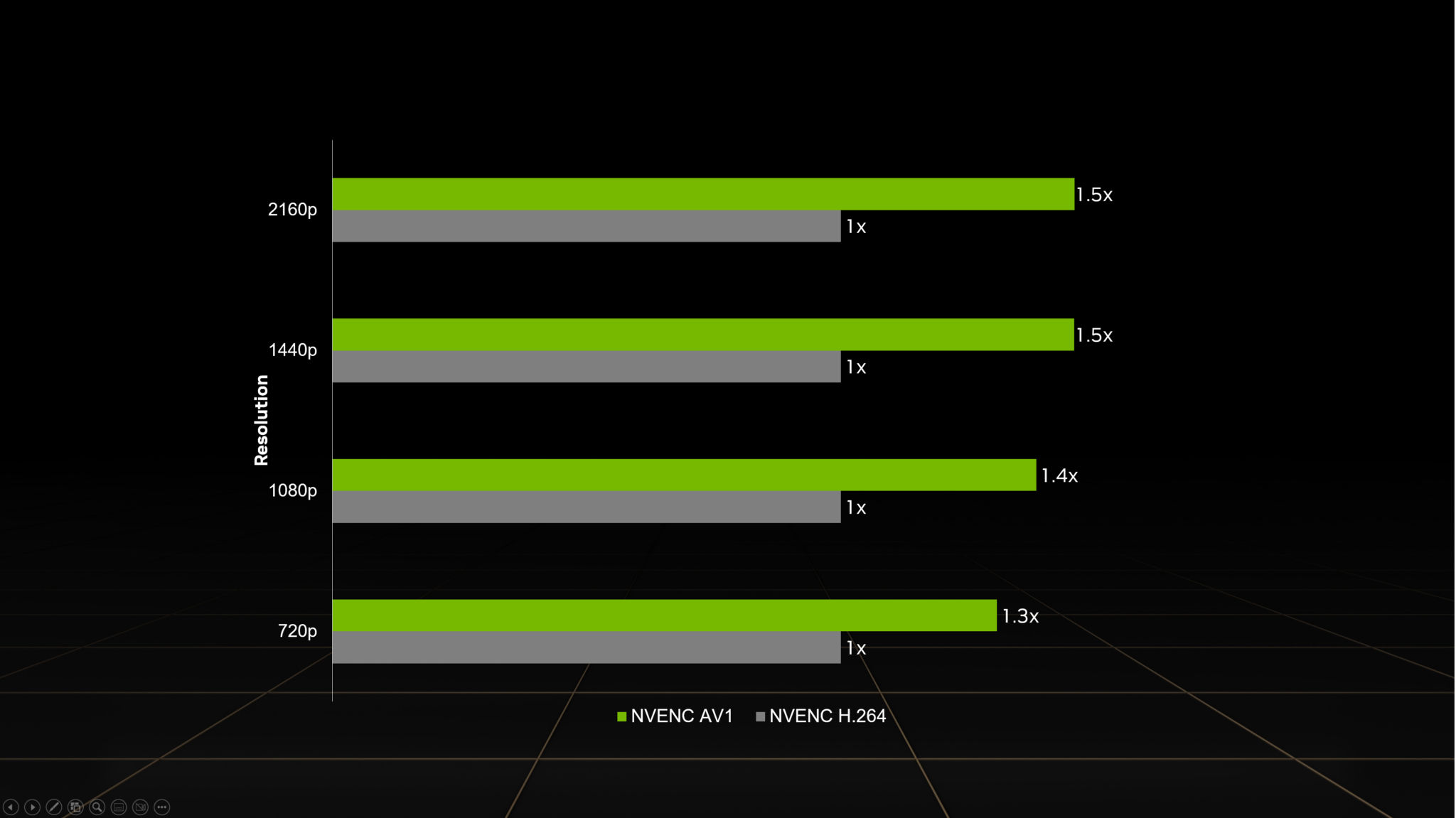
This reduces the upload bandwidth needed to stream, a common limitation from streaming services and internet service providers. At higher resolutions, AV1 encoding is even more efficient. For example, AV1 enables streaming 4K at 60 frames per second with 10 Mbps upload bandwidth — down from 20 Mbps with H.264 — making 4K60 streaming available to a wider audience.
AV1 — The New Standard
As a founding member of the Alliance for Open Media, NVIDIA has worked closely with industry titans in developing the AV1 codec. This work was necessitated by gamers and online content creators who pushed the boundaries of old formats that were defined roughly 20 years ago. The previous standard for livestreaming, H.264, usually maxed out with 1080p at 60 fps at the commonly used bitrates of 6-8 Mbps, and often produced blocky, grainy images.
AV1’s increased efficiency enables streaming higher-quality images, allowing creators to stream at higher resolutions with smoother frame rates. Even in network-limited environments, streamers can now reap the benefits of high-quality video shared with their audience.
Support for AV1 on YouTube comes through the recent update to RTMP. The enhanced protocol also adds support for HEVC streaming, bringing new formats to users on the existing low-latency protocol they use for H.264 streaming. Enhanced RTMP ingestion has been released as a beta feature on YouTube.
Learn how to configure OBS Studio for streaming AV1 with GeForce RTX 40 Series GPUs in the OBS setup guide.
Better Streams With NVENC, NVIDIA Broadcast
GeForce RTX 40 Series GPUs usher in a new era of high-quality streaming with AV1 encoding support on the eighth-generation NVENC. A boon to streamers, NVENC offloads compute-intensive encoding tasks from the CPU to dedicated hardware on the GPU.
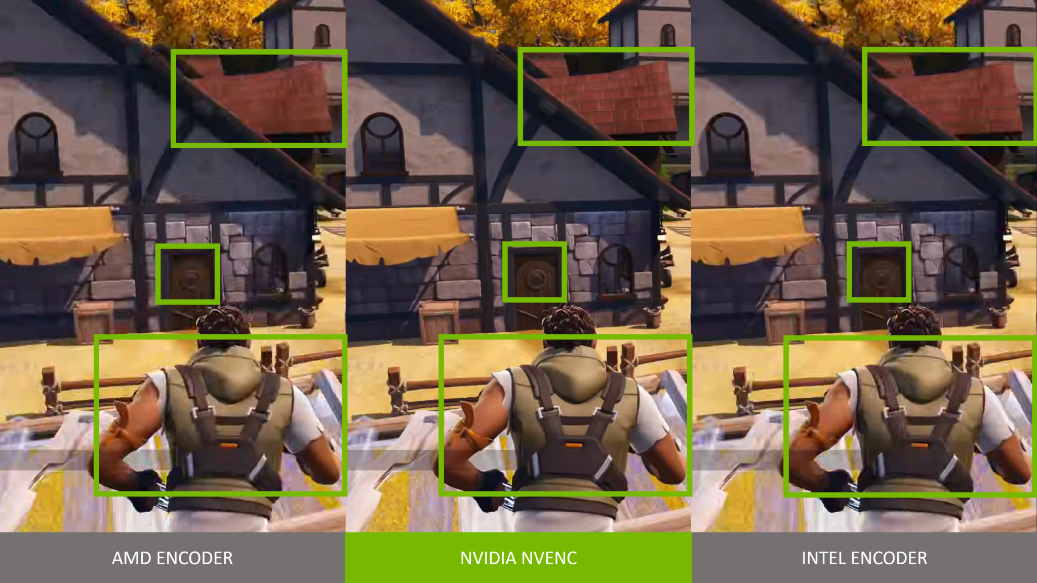
Designed to support the rigors of professional content creators, NVENC preserves video quality with a higher accuracy than competitive encoders. GeForce RTX users can stream higher-quality images at the same bitrate as competitive products or encode at a lower bitrate while maintaining a similar picture quality.
NVIDIA Broadcast, part of the exclusive NVIDIA Studio suite of software, transforms any room into a home studio. Livestreams, voice chats and video calls look and sound better with powerful AI effects like eye contact, noise and room echo removal, virtual background and more.
Follow NVIDIA Studio on Instagram, Twitter and Facebook. Access tutorials on the Studio YouTube channel and get updates directly in your inbox by subscribing to the Studio newsletter.
1 Source: 4K60 AV1 encoded video with AMD 7900 XT, GeForce RTX 4080 and Intel Arc 770 with OBS Studio default settings at 12Mbps
Hosting ML Models on Amazon SageMaker using Triton: XGBoost, LightGBM, and Treelite Models
One of the most popular models available today is XGBoost. With the ability to solve various problems such as classification and regression, XGBoost has become a popular option that also falls into the category of tree-based models. In this post, we dive deep to see how Amazon SageMaker can serve these models using NVIDIA Triton Inference Server. Real-time inference workloads can have varying levels of requirements and service level agreements (SLAs) in terms of latency and throughput, and can be met using SageMaker real-time endpoints.
SageMaker provides single model endpoints, which allow you to deploy a single machine learning (ML) model against a logical endpoint. For other use cases, you can choose to manage cost and performance using multi-model endpoints, which allow you to specify multiple models to host behind a logical endpoint. Regardless of the option the you choose, SageMaker endpoints allow a scalable mechanism for even the most demanding enterprise customers while providing value in a plethora of features, including shadow variants, auto scaling, and native integration with Amazon CloudWatch (for more information, refer to CloudWatch Metrics for Multi-Model Endpoint Deployments).
Triton supports various backends as engines to support the running and serving of various ML models for inference. For any Triton deployment, it’s crucial to know how the backend behavior impacts your workloads and what to expect so that you can be successful. In this post, we help you understand the Forest Inference Library (FIL) backend, which is supported by Triton on SageMaker, so that you can make an informed decision for your workloads and get the best performance and cost optimization possible.
Deep dive into the FIL backend
Triton supports the FIL backend to serve tree models, such as XGBoost, LightGBM, scikit-learn Random Forest, RAPIDS cuML Random Forest, and any other model supported by Treelite. These models have long been used for solving problems such as classification or regression. Although these types of models have traditionally run on CPUs, the popularity of these models and inference demands have led to various techniques to increase inference performance. The FIL backend utilizes many of these techniques by using cuML constructs and is built on C++ and the CUDA core library to optimize inference performance on GPU accelerators.
The FIL backend uses cuML’s libraries to use CPU or GPU cores to accelerate learning. In order to use these processors, data is referenced from host memory (for example, NumPy arrays) or GPU arrays (uDF, Numba, cuPY, or any library that supports the __cuda_array_interface__) API. After the data is staged in memory, the FIL backend can run processing across all the available CPU or GPU cores.
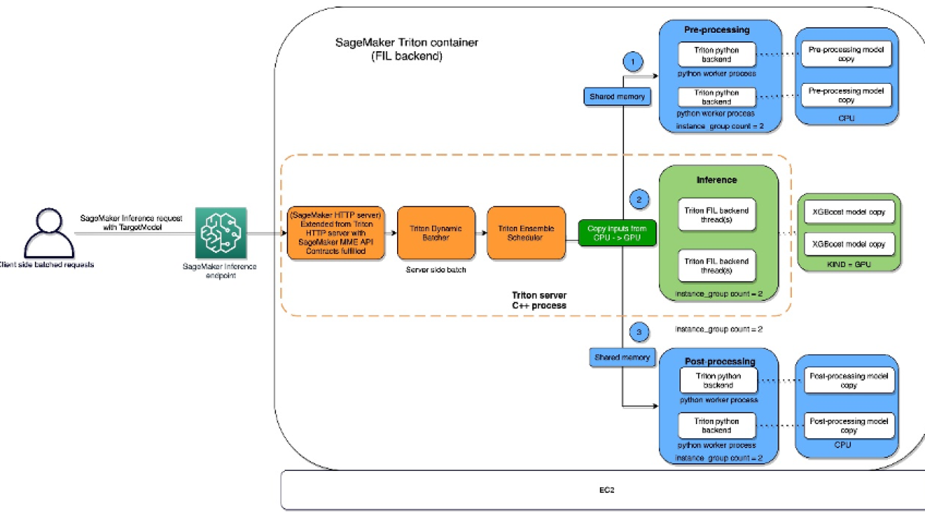
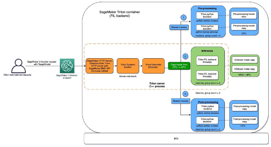
The FIL backend threads can communicate with each other without utilizing shared memory of the host, but in ensemble workloads, host memory should be considered. The following diagram shows an ensemble scheduler runtime architecture where you have the ability to fine-tune the memory areas, including CPU addressable shared memory that is used for inter-process communication between Triton (C++) and the Python process (Python backend) for exchanging tensors (input/output) with the FIL backend.
Triton Inference Server provides configurable options for developers to tune their workloads and optimize model performance. The configuration dynamic_batching allows Triton to hold client-side requests and batch them on the server side in order to efficiently use FIL’s parallel computation to inference the entire batch together. The option max_queue_delay_microseconds offers a fail-safe control of how long Triton waits to form a batch.
There are a number of other FIL-specific options available that impact performance and behavior. We suggest starting with storage_type. When running the backend on GPU, FIL creates a new memory/data structure that is a representation of the tree for which FIL can impact performance and footprint. This is configurable via the environment parameter storage_type, which has the options dense, sparse, and auto. Choosing the dense option will consume more GPU memory and doesn’t always result in better performance, so it’s best to check. In contrast, the sparse option will consume less GPU memory and can possibly perform as well or better than dense. Choosing auto will cause the model to default to dense unless doing so will consume significantly more GPU memory than sparse.
When it comes to model performance, you might consider emphasizing the threads_per_tree option. One thing that you may overserve in real-world scenarios is that threads_per_tree can have a bigger impact on throughput than any other parameter. Setting it to any power of 2 from 1–32 is legitimate. The optimal value is hard to predict for this parameter, but when the server is expected to deal with higher load or process larger batch sizes, it tends to benefit from a larger value than when it’s processing a few rows at a time.
Another parameter to be aware of is algo, which is also available if you’re running on GPU. This parameter determines the algorithm that’s used to process the inference requests. The options supported for this are ALGO_AUTO, NAIVE, TREE_REORG, and BATCH_TREE_REORG. These options determine how nodes within a tree are organized and can also result in performance gains. The ALGO_AUTO option defaults to NAIVE for sparse storage and BATCH_TREE_REORG for dense storage.
Lastly, FIL comes with Shapley explainer, which can be activated by using the treeshap_output parameter. However, you should keep in mind that Shapley outputs hurt performance due to its output size.
Model format
There is currently no standard file format to store forest-based models; every framework tends to define its own format. In order to support multiple input file formats, FIL imports data using the open-source Treelite library. This enables FIL to support models trained in popular frameworks, such as XGBoost and LightGBM. Note that the format of the model that you’re providing must be set in the model_type configuration value specified in the config.pbtxt file.
Config.pbtxt
Each model in a model repository must include a model configuration that provides the required and optional information about the model. Typically, this configuration is provided in a config.pbtxt file specified as ModelConfig protobuf. To learn more about the config settings, refer to Model Configuration. The following are some of the model configuration parameters:
- max_batch_size – This determines the maximum batch size that can be passed to this model. In general, the only limit on the size of batches passed to a FIL backend is the memory available with which to process them. For GPU runs, the available memory is determined by the size of Triton’s CUDA memory pool, which can be set via a command line argument when starting the server.
- input – Options in this section tell Triton the number of features to expect for each input sample.
- output – Options in this section tell Triton how many output values there will be for each sample. If the
predict_probaoption is set to true, then a probability value will be returned for each class. Otherwise, a single value will be returned, indicating the class predicted for the given sample. - instance_group – This determines how many instances of this model will be created and whether they will use GPU or CPU.
- model_type – This string indicates what format the model is in (
xgboost_jsonin this example, butxgboost,lightgbm, andtl_checkpointare valid formats as well). - predict_proba – If set to true, probability values will be returned for each class rather than just a class prediction.
- output_class – This is set to true for classification models and false for regression models.
- threshold – This is a score threshold for determining classification. When
output_classis set to true, this must be provided, although it won’t be used ifpredict_probais also set to true. - storage_type – In general, using AUTO for this setting should meet most use cases. If AUTO storage is selected, FIL will load the model using either a sparse or dense representation based on the approximate size of the model. In some cases, you may want to explicitly set this to SPARSE in order to reduce the memory footprint of large models.
Triton Inference Server on SageMaker
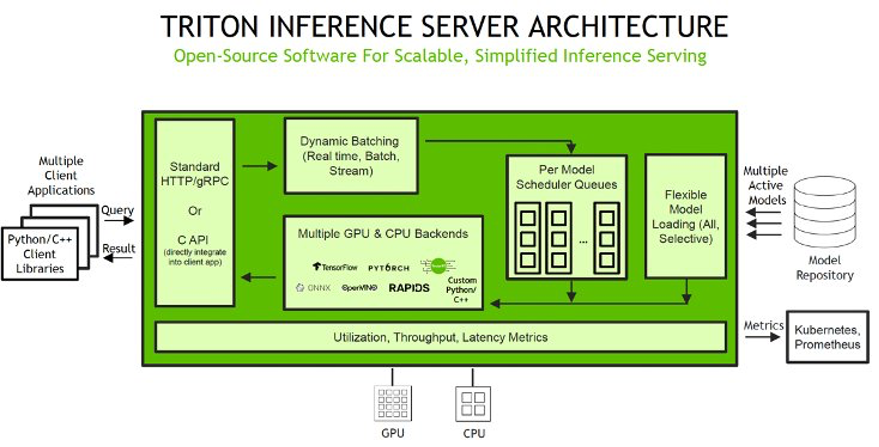
SageMaker allows you to deploy both single model and multi-model endpoints with NVIDIA Triton Inference Server. The following figure shows the Triton Inference Server high-level architecture. The model repository is a file system-based repository of the models that Triton will make available for inferencing. Inference requests arrive at the server and are routed to the appropriate per-model scheduler. Triton implements multiple scheduling and batching algorithms that can be configured on a model-by-model basis. Each model’s scheduler optionally performs batching of inference requests and then passes the requests to the backend corresponding to the model type. The backend performs inferencing using the inputs provided in the batched requests to produce the requested outputs. The outputs are then returned.
When configuring your auto scaling groups for SageMaker endpoints, you may want to consider SageMakerVariantInvocationsPerInstance as the primary criteria to determine the scaling characteristics of your auto scaling group. In addition, depending on whether your models are running on GPU or CPU, you may also consider using CPUUtilization or GPUUtilization as additional criteria. Note that for single model endpoints, because the models deployed are all the same, it’s fairly straightforward to set proper policies to meet your SLAs. For multi-model endpoints, we recommend deploying similar models behind a given endpoint to have more steady predictable performance. In use cases where models of varying sizes and requirements are used, you may want to separate those workloads across multiple multi-model endpoints or spend some time fine-tuning your auto scaling group policy to obtain the best cost and performance balance.
For a list of NVIDIA Triton Deep Learning Containers (DLCs) supported by SageMaker inference, refer to Available Deep Learning Containers Images.
SageMaker notebook walkthrough
ML applications are complex and can often require data preprocessing. In this notebook, we dive into how to deploy a tree-based ML model like XGBoost using the FIL backend in Triton on a SageMaker multi-model endpoint. We also cover how to implement a Python-based data preprocessing inference pipeline for your model using the ensemble feature in Triton. This will allow us to send in the raw data from the client side and have both data preprocessing and model inference happen in a Triton SageMaker endpoint for optimal inference performance.
Triton model ensemble feature
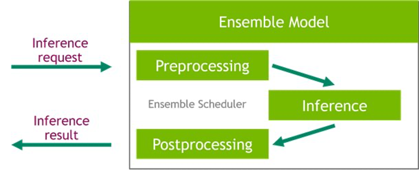
Triton Inference Server greatly simplifies the deployment of AI models at scale in production. Triton Inference Server comes with a convenient solution that simplifies building preprocessing and postprocessing pipelines. The Triton Inference Server platform provides the ensemble scheduler, which is responsible for pipelining models participating in the inference process while ensuring efficiency and optimizing throughput. Using ensemble models can avoid the overhead of transferring intermediate tensors and minimize the number of requests that must be sent to Triton.
In this notebook, we show how to use the ensemble feature for building a pipeline of data preprocessing with XGBoost model inference, and you can extrapolate from it to add custom postprocessing to the pipeline.
Set up the environment
We begin by setting up the required environment. We install the dependencies required to package our model pipeline and run inferences using Triton Inference Server. We also define the AWS Identity and Access Management (IAM) role that will give SageMaker access to the model artifacts and the NVIDIA Triton Amazon Elastic Container Registry (Amazon ECR) image. See the following code:
Create a Conda environment for preprocessing dependencies
The Python backend in Triton requires us to use a Conda environment for any additional dependencies. In this case, we use the Python backend to preprocess the raw data before feeding it into the XGBoost model that is running in the FIL backend. Even though we originally used RAPIDS cuDF and cuML to do the data preprocessing, here we use Pandas and scikit-learn as preprocessing dependencies during inference. We do this for three reasons:
- We show how to create a Conda environment for your dependencies and how to package it in the format expected by Triton’s Python backend.
- By showing the preprocessing model running in the Python backend on the CPU while the XGBoost runs on the GPU in the FIL backend, we illustrate how each model in Triton’s ensemble pipeline can run on a different framework backend as well as different hardware configurations.
- It highlights how the RAPIDS libraries (cuDF, cuML) are compatible with their CPU counterparts (Pandas, scikit-learn). For example, we can show how
LabelEncoderscreated in cuML can be used in scikit-learn and vice versa.
We follow the instructions from the Triton documentation for packaging preprocessing dependencies (scikit-learn and Pandas) to be used in the Python backend as a Conda environment TAR file. The bash script create_prep_env.sh creates the Conda environment TAR file, then we move it into the preprocessing model directory. See the following code:
After we run the preceding script, it generates preprocessing_env.tar.gz, which we copy to the preprocessing directory:
Set up preprocessing with the Triton Python backend
For preprocessing, we use Triton’s Python backend to perform tabular data preprocessing (categorical encoding) during inference for raw data requests coming into the server. For more information about the preprocessing that was done during training, refer to the training notebook.
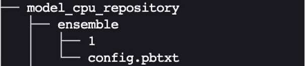
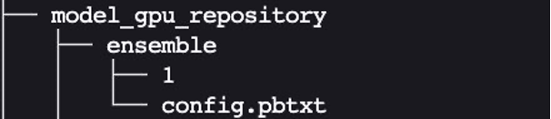
The Python backend enables preprocessing, postprocessing, and any other custom logic to be implemented in Python and served with Triton. Using Triton on SageMaker requires us to first set up a model repository folder containing the models we want to serve. We have already set up a model for Python data preprocessing called preprocessing in cpu_model_repository and gpu_model_repository.
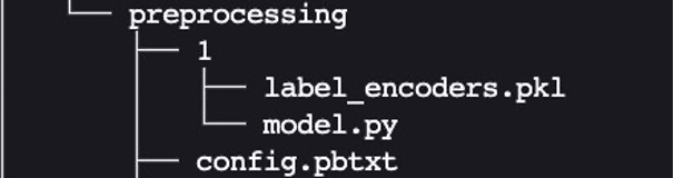
Triton has specific requirements for model repository layout. Within the top-level model repository directory, each model has its own subdirectory containing the information for the corresponding model. Each model directory in Triton must have at least one numeric subdirectory representing a version of the model. The value 1 represents version 1 of our Python preprocessing model. Each model is run by a specific backend, so within each version subdirectory there must be the model artifact required by that backend. For this example, we use the Python backend, which requires the Python file you’re serving to be called model.py, and the file needs to implement certain functions. If we were using a PyTorch backend, a model.pt file would be required, and so on. For more details on naming conventions for model files, refer to Model Files.
The model.py Python file we use here implements all the tabular data preprocessing logic to convert raw data into features that can be fed into our XGBoost model.
Every Triton model must also provide a config.pbtxt file describing the model configuration. To learn more about the config settings, refer to Model Configuration. Our config.pbtxt file specifies the backend as python and all the input columns for raw data along with preprocessed output, which consists of 15 features. We also specify we want to run this Python preprocessing model on the CPU. See the following code:
Set up a tree-based ML model for the FIL backend
Next, we set up the model directory for a tree-based ML model like XGBoost, which will be using the FIL backend.
The expected layout for cpu_memory_repository and gpu_memory_repository are similar to the one we showed earlier.
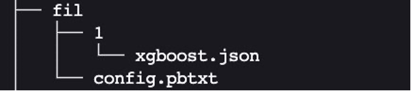
Here, FIL is the name of the model. We can give it a different name like xgboost if we want to. 1 is the version subdirectory, which contains the model artifact. In this case, it’s the xgboost.json model that we saved. Let’s create this expected layout:
We need to have the configuration file config.pbtxt describing the model configuration for the tree-based ML model, so that the FIL backend in Triton can understand how to serve it. For more information, refer to the latest generic Triton configuration options and the configuration options specific to the FIL backend. We focus on just a few of the most common and relevant options in this example.
Create config.pbtxt for model_cpu_repository:
Similarly, set up config.pbtxt for model_gpu_repository (note the difference is USE_GPU = True):
Set up an inference pipeline of the data preprocessing Python backend and FIL backend using ensembles
Now we’re ready to set up the inference pipeline for data preprocessing and tree-based model inference using an ensemble model. An ensemble model represents a pipeline of one or more models and the connection of input and output tensors between those models. Here we use the ensemble model to build a pipeline of data preprocessing in the Python backend followed by XGBoost in the FIL backend.
The expected layout for the ensemble model directory is similar to the ones we showed previously:
We created the ensemble model’s config.pbtxt following the guidance in Ensemble Models. Importantly, we need to set up the ensemble scheduler in config.pbtxt, which specifies the data flow between models within the ensemble. The ensemble scheduler collects the output tensors in each step, and provides them as input tensors for other steps according to the specification.
Package the model repository and upload to Amazon S3
Finally, we end up with the following model repository directory structure, containing a Python preprocessing model and its dependencies along with the XGBoost FIL model and the model ensemble.
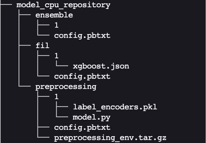
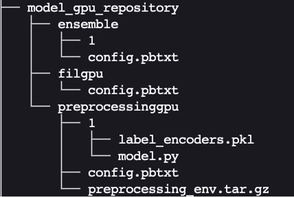
We package the directory and its contents as model.tar.gz for uploading to Amazon Simple Storage Service (Amazon S3). We have two options in this example: using a CPU-based instance or a GPU-based instance. A GPU-based instance is more suitable when you need higher processing power and want to use CUDA cores.
Create and upload the model package for a CPU-based instance (optimized for CPU) with the following code:
Create and upload the model package for a GPU-based instance (optimized for GPU) with the following code:
Create a SageMaker endpoint
We now have the model artifacts stored in an S3 bucket. In this step, we can also provide the additional environment variable SAGEMAKER_TRITON_DEFAULT_MODEL_NAME, which specifies the name of the model to be loaded by Triton. The value of this key should match the folder name in the model package uploaded to Amazon S3. This variable is optional in the case of a single model. In the case of ensemble models, this key has to be specified for Triton to start up in SageMaker.
Additionally, you can set SAGEMAKER_TRITON_BUFFER_MANAGER_THREAD_COUNT and SAGEMAKER_TRITON_THREAD_COUNT for optimizing the thread counts.
We use the preceding model to create an endpoint configuration where we can specify the type and number of instances we want in the endpoint
We use this endpoint configuration to create a SageMaker endpoint and wait for the deployment to finish. With SageMaker MMEs, we have the option to host multiple ensemble models by repeating this process, but we stick with one deployment for this example:
The status will change to InService when the deployment is successful.
Invoke your model hosted on the SageMaker endpoint
After the endpoint is running, we can use some sample raw data to perform inference using JSON as the payload format. For the inference request format, Triton uses the KFServing community standard inference protocols. See the following code:
The notebook referred in the blog can be found in the GitHub repository.
Best practices
In addition to the options to fine-tune the settings of the FIL backend we mentioned earlier, data scientists can also ensure that the input data for the backend is optimized for processing by the engine. Whenever possible, input data in row-major format into the GPU array. Other formats will require internal conversion and take up cycles, decreasing performance.
Due to the way FIL data structures are maintained in GPU memory, be mindful of the tree depth. The deeper the tree depth, the larger your GPU memory footprint will be.
Use the instance_group_count parameter to add worker processes and increase the throughput of the FIL backend, which will result in larger CPU and GPU memory consumption. In addition, consider SageMaker-specific variables that are available to increase the throughput, such as HTTP threads, HTTP buffer size, batch size, and max delay.
Conclusion
In this post, we dove deep into the FIL backend that Triton Inference Server supports on SageMaker. This backend provides for both CPU and GPU acceleration of your tree-based models such as the popular XGBoost algorithm. There are many options to consider to get the best performance for inference, such as batch sizes, data input formats, and other factors that can be tuned to meet your needs. SageMaker allows you to use this capability with single and multi-model endpoints to balance of performance and cost savings.
We encourage you to take the information in this post and see if SageMaker can meet your hosting needs to serve tree-based models, meeting your requirements for cost reduction and workload performance.
The notebook referenced in this post can be found in the SageMaker examples GitHub repository. Furthermore, you can find the latest documentation on the FIL backend on GitHub.
About the Authors
 Raghu Ramesha is an Senior ML Solutions Architect with the Amazon SageMaker Service team. He focuses on helping customers build, deploy, and migrate ML production workloads to SageMaker at scale. He specializes in machine learning, AI, and computer vision domains, and holds a master’s degree in Computer Science from UT Dallas. In his free time, he enjoys traveling and photography.
 James Park is a Solutions Architect at Amazon Web Services. He works with Amazon.com to design, build, and deploy technology solutions on AWS, and has a particular interest in AI and machine learning. In his spare time he enjoys seeking out new cultures, new experiences, and staying up to date with the latest technology trends.
 Dhawal Patel is a Principal Machine Learning Architect at AWS. He has worked with organizations ranging from large enterprises to mid-sized startups on problems related to distributed computing and artificial intelligence. He focuses on deep learning, including NLP and computer vision domains. He helps customers achieve high-performance model inference on Amazon SageMaker.
 Jiahong Liu is a Solution Architect on the Cloud Service Provider team at NVIDIA. He assists clients in adopting machine learning and AI solutions that leverage NVIDIA accelerated computing to address their training and inference challenges. In his leisure time, he enjoys origami, DIY projects, and playing basketball.
 Kshitiz Gupta is a Solutions Architect at NVIDIA. He enjoys educating cloud customers about the GPU AI technologies NVIDIA has to offer and assisting them with accelerating their machine learning and deep learning applications. Outside of work, he enjoys running, hiking and wildlife watching.
ICLR: Why does deep learning work, and what are its limits?
Two recent trends in the theory of deep learning are examinations of the double-descent phenomenon and more-realistic approaches to neural kernel methods.Read More