Using audio and text embeddings jointly for Keyword Spotting (KWS) has shown high-quality results, but the key challenge of how to semantically align two embeddings for multi-word keywords of different sequence lengths remains largely unsolved. In this paper, we propose an audio-text-based end-to-end model architecture for flexible keyword spotting (KWS), which builds upon learned audio and text embeddings. Our architecture uses a novel dynamic programming-based algorithm, Dynamic Sequence Partitioning (DSP), to optimally partition the audio sequence into the same length as the…Apple Machine Learning Research
Semi-Supervised and Long-Tailed Object Detection with CascadeMatch
This paper focuses on long-tailed object detection in the semi-supervised learning setting, which poses realistic challenges, but has rarely been studied in the literature. We propose a novel pseudo-labeling-based detector called CascadeMatch. Our detector features a cascade network architecture, which has multi-stage detection heads with progressive confidence thresholds. To avoid manually tuning the thresholds, we design a new adaptive pseudo-label mining mechanism to automatically identify suitable values from data. To mitigate confirmation bias, where a model is negatively reinforced by…Apple Machine Learning Research
Near-Optimal Algorithms for Private Online Optimization in the Realizable Regime
*=Equal Contributors
We consider online learning problems in the realizable setting, where there is a zero-loss solution, and propose new Differentially Private (DP) algorithms that obtain near-optimal regret bounds. For the problem of online prediction from experts, we design new algorithms that obtain near-optimal regret where is the number of experts. This significantly improves over the best existing regret bounds for the DP non-realizable setting which are . We also develop an adaptive algorithm for the small-loss setting with regret where is the total loss of the best expert…Apple Machine Learning Research
Approximate Nearest Neighbor Phrase Mining for Contextual Speech Recognition
This paper presents an extension to train end-to-end Context-Aware Transformer Transducer ( CATT ) models by using a simple, yet efficient method of mining hard negative phrases from the latent space of the context encoder. During training, given a reference query, we mine a number of similar phrases using approximate nearest neighbour search. These sampled phrases are then used as negative examples in the context list alongside random and ground truth contextual information. By including approximate nearest neighbour phrases (ANN-P) in the context list, we encourage the learned representation…Apple Machine Learning Research
RoomDreamer: Text-Driven 3D Indoor Scene Synthesis with Coherent Geometry and Texture
The techniques for 3D indoor scene capturing are widely used, but the meshes produced leave much to be desired. In this paper, we propose “RoomDreamer”, which leverages powerful natural language to synthesize a new room with a different style. Unlike existing image synthesis methods, our work addresses the challenge of synthesizing both geometry and texture aligned to the input scene structure and prompt simultaneously. The key insight is that a scene should be treated as a whole, taking into account both scene texture and geometry. The proposed framework consists of two significant…Apple Machine Learning Research
Host ML models on Amazon SageMaker using Triton: ONNX Models
ONNX (Open Neural Network Exchange) is an open-source standard for representing deep learning models widely supported by many providers. ONNX provides tools for optimizing and quantizing models to reduce the memory and compute needed to run machine learning (ML) models. One of the biggest benefits of ONNX is that it provides a standardized format for representing and exchanging ML models between different frameworks and tools. This allows developers to train their models in one framework and deploy them in another without the need for extensive model conversion or retraining. For these reasons, ONNX has gained significant importance in the ML community.
In this post, we showcase how to deploy ONNX-based models for multi-model endpoints (MMEs) that use GPUs. This is a continuation of the post Run multiple deep learning models on GPU with Amazon SageMaker multi-model endpoints, where we showed how to deploy PyTorch and TensorRT versions of ResNet50 models on Nvidia’s Triton Inference server. In this post, we use the same ResNet50 model in ONNX format along with an additional natural language processing (NLP) example model in ONNX format to show how it can be deployed on Triton. Furthermore, we benchmark the ResNet50 model and see the performance benefits that ONNX provides when compared to PyTorch and TensorRT versions of the same model, using the same input.

ONNX Runtime
ONNX Runtime is a runtime engine for ML inference designed to optimize the performance of models across multiple hardware platforms, including CPUs and GPUs. It allows the use of ML frameworks like PyTorch and TensorFlow. It facilitates performance tuning to run models cost-efficiently on the target hardware and has support for features like quantization and hardware acceleration, making it one of the ideal choices for deploying efficient, high-performance ML applications. For examples of how ONNX models can be optimized for Nvidia GPUs with TensorRT, refer to TensorRT Optimization (ORT-TRT) and ONNX Runtime with TensorRT optimization.
The Amazon SageMaker Triton container flow is depicted in the following diagram.
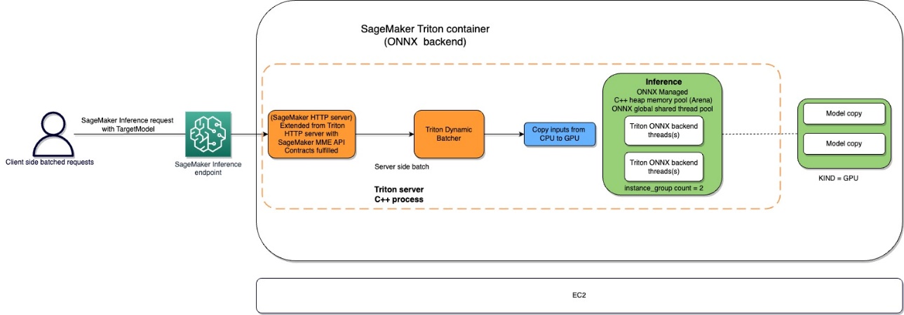
Users can send an HTTPS request with the input payload for real-time inference behind a SageMaker endpoint. The user can specify a TargetModel header that contains the name of the model that the request in question is destined to invoke. Internally, the SageMaker Triton container implements an HTTP server with the same contracts as mentioned in How Containers Serve Requests. It has support for dynamic batching and supports all the backends that Triton provides. Based on the configuration, the ONNX runtime is invoked and the request is processed on CPU or GPU as predefined in the model configuration provided by the user.
Solution overview
To use the ONNX backend, complete the following steps:
- Compile the model to ONNX format.
- Configure the model.
- Create the SageMaker endpoint.
Prerequisites
Ensure that you have access to an AWS account with sufficient AWS Identity and Access Management IAM permissions to create a notebook, access an Amazon Simple Storage Service (Amazon S3) bucket, and deploy models to SageMaker endpoints. See Create execution role for more information.
Compile the model to ONNX format
The transformers library provides for convenient method to compile the PyTorch model to ONNX format. The following code achieves the transformations for the NLP model:
Exporting models (either PyTorch or TensorFlow) is easily achieved through the conversion tool provided as part of the Hugging Face transformers repository.
The following is what happens under the hood:
- Allocate the model from transformers (PyTorch or TensorFlow).
- Forward dummy inputs through the model. This way, ONNX can record the set of operations run.
- The transformers inherently take care of dynamic axes when exporting the model.
- Save the graph along with the network parameters.
A similar mechanism is followed for the computer vision use case from the torchvision model zoo:
Configure the model
In this section, we configure the computer vision and NLP model. We show how to create a ResNet50 and RoBERTA large model that has been pre-trained for deployment on a SageMaker MME by utilizing Triton Inference Server model configurations. The ResNet50 notebook is available on GitHub. The RoBERTA notebook is also available on GitHub. For ResNet50, we use the Docker approach to create an environment that already has all the dependencies required to build our ONNX model and generate the model artifacts needed for this exercise. This approach makes it much easier to share dependencies and create the exact environment that is needed to accomplish this task.
The first step is to create the ONNX model package per the directory structure specified in ONNX Models. Our aim is to use the minimal model repository for a ONNX model contained in a single file as follows:
Next, we create the model configuration file that describes the inputs, outputs, and backend configurations for the Triton Server to pick up and invoke the appropriate kernels for ONNX. This file is known as config.pbtxt and is shown in the following code for the RoBERTA use case. Note that the BATCH dimension is omitted from the config.pbtxt. However, when sending the data to the model, we include the batch dimension. The following code also shows how you can add this feature with model configuration files to set dynamic batching with a preferred batch size of 5 for the actual inference. With the current settings, the model instance is invoked instantly when the preferred batch size of 5 is met or the delay time of 100 microseconds has elapsed since the first request reached the dynamic batcher.
The following is the similar configuration file for the computer vision use case:
Create the SageMaker endpoint
We use the Boto3 APIs to create the SageMaker endpoint. For this post, we show the steps for the RoBERTA notebook, but these are common steps and will be the same for the ResNet50 model as well.
Create a SageMaker model
We now create a SageMaker model. We use the Amazon Elastic Container Registry (Amazon ECR) image and the model artifact from the previous step to create the SageMaker model.
Create the container
To create the container, we pull the appropriate image from Amazon ECR for Triton Server. SageMaker allows us to customize and inject various environment variables. Some of the key features are the ability to set the BATCH_SIZE; we can set this per model in the config.pbtxt file, or we can define a default value here. For models that can benefit from larger shared memory size, we can set those values under SHM variables. To enable logging, set the log verbose level to true. We use the following code to create the model to use in our endpoint:
Create a SageMaker endpoint
You can use any instances with multiple GPUs for testing. In this post, we use a g4dn.4xlarge instance. We don’t set the VolumeSizeInGB parameters because this instance comes with local instance storage. The VolumeSizeInGB parameter is applicable to GPU instances supporting the Amazon Elastic Block Store (Amazon EBS) volume attachment. We can leave the model download timeout and container startup health check at the default values. For more details, refer to CreateEndpointConfig.
Lastly, we create a SageMaker endpoint:
Invoke the model endpoint
This is a generative model, so we pass in the input_ids and attention_mask to the model as part of the payload. The following code shows how to create the tensors:
We now create the appropriate payload by ensuring the data type matches what we configured in the config.pbtxt. This also give us the tensors with the batch dimension included, which is what Triton expects. We use the JSON format to invoke the model. Triton also provides a native binary invocation method for the model.
Note the TargetModel parameter in the preceding code. We send the name of the model to be invoked as a request header because this is a multi-model endpoint, therefore we can invoke multiple models at runtime on an already deployed inference endpoint by changing this parameter. This shows the power of multi-model endpoints!
To output the response, we can use the following code:
ONNX for performance tuning
The ONNX backend uses C++ arena memory allocation. Arena allocation is a C++-only feature that helps you optimize your memory usage and improve performance. Memory allocation and deallocation constitutes a significant fraction of CPU time spent in protocol buffers code. By default, new object creation performs heap allocations for each object, each of its sub-objects, and several field types, such as strings. These allocations occur in bulk when parsing a message and when building new messages in memory, and associated deallocations happen when messages and their sub-object trees are freed.
Arena-based allocation has been designed to reduce this performance cost. With arena allocation, new objects are allocated out of a large piece of pre-allocated memory called the arena. Objects can all be freed at once by discarding the entire arena, ideally without running destructors of any contained object (though an arena can still maintain a destructor list when required). This makes object allocation faster by reducing it to a simple pointer increment, and makes deallocation almost free. Arena allocation also provides greater cache efficiency: when messages are parsed, they are more likely to be allocated in continuous memory, which makes traversing messages more likely to hit hot cache lines. The downside of arena-based allocation is the C++ heap memory will be over-allocated and stay allocated even after the objects are deallocated. This might lead to out of memory or high CPU memory usage. To achieve the best of both worlds, we use the following configurations provided by Triton and ONNX:
- arena_extend_strategy – This parameter refers to the strategy used to grow the memory arena with regards to the size of the model. We recommend setting the value to 1 (=
kSameAsRequested), which is not a default value. The reasoning is as follows: the drawback of the default arena extend strategy (kNextPowerOfTwo) is that it might allocate more memory than needed, which could be a waste. As the name suggests,kNextPowerOfTwo(the default) extends the arena by a power of 2, whereaskSameAsRequestedextends by a size that is the same as the allocation request each time.kSameAsRequestedis suited for advanced configurations where you know the expected memory usage in advance. In our testing, because we know the size of models is a constant value, we can safely choosekSameAsRequested. - gpu_mem_limit – We set the value to the CUDA memory limit. To use all possible memory, pass in the maximum
size_t. It defaults toSIZE_MAXif nothing is specified. We recommend keeping it as default. - enable_cpu_mem_arena – This enables the memory arena on CPU. The arena may pre-allocate memory for future usage. Set this option to
falseif you don’t want it. The default isTrue. If you disable the arena, heap memory allocation will take time, so inference latency will increase. In our testing, we left it as default. - enable_mem_pattern – This parameter refers to the internal memory allocation strategy based on input shapes. If the shapes are constant, we can enable this parameter to generate a memory pattern for the future and save some allocation time, making it faster. Use 1 to enable the memory pattern and 0 to disable. It’s recommended to set this to 1 when the input features are expected to be the same. The default value is 1.
- do_copy_in_default_stream – In the context of the CUDA execution provider in ONNX, a compute stream is a sequence of CUDA operations that are run asynchronously on the GPU. The ONNX runtime schedules operations in different streams based on their dependencies, which helps minimize the idle time of the GPU and achieve better performance. We recommend using the default setting of 1 for using the same stream for copying and compute; however, you can use 0 for using separate streams for copying and compute, which might result in the device pipelining the two activities. In our testing of the ResNet50 model, we used both 0 and 1 but couldn’t find any appreciable difference between the two in terms of performance and memory consumption of the GPU device.
- Graph optimization – The ONNX backend for Triton supports several parameters that help fine-tune the model size as well as runtime performance of the deployed model. When the model is converted to the ONNX representation (the first box in the following diagram at the IR stage), the ONNX runtime provides graph optimizations at three levels: basic, extended, and layout optimizations. You can activate all levels of graph optimizations by adding the following parameters in the model configuration file:
- cudnn_conv_algo_search – Because we’re using CUDA-based Nvidia GPUs in our testing, for our computer vision use case with the ResNet50 model, we can use the CUDA execution provider-based optimization at the fourth layer in the following diagram with the
cudnn_conv_algo_searchparameter. The default option is exhaustive (0), but when we changed this configuration to1 – HEURISTIC, we saw the model latency in steady state reduce to 160 milliseconds. The reason this happens is because the ONNX runtime invokes the lighter weight cudnnGetConvolutionForwardAlgorithm_v7 forward pass and therefore reduces latency with adequate performance. - Run mode – The next step is selecting the correct execution_mode at layer 5 in the following diagram. This parameter controls whether you want to run operators in your graph sequentially or in parallel. Usually when the model has many branches, setting this option to
ExecutionMode.ORT_PARALLEL(1) will give you better performance. In the scenario where your model has many branches in its graph, setting the run mode to parallel will help with better performance. The default mode is sequential, so you can enable this to suit your needs.
For a deeper understanding of the opportunities for performance tuning in ONNX, refer to the following figure.

Benchmark numbers and performance tuning
By turning on the graph optimizations, cudnn_conv_algo_search, and parallel run mode parameters in our testing of the ResNet50 model, we saw the cold start time of the ONNX model graph reduce from 4.4 seconds to 1.61 seconds. An example of a complete model configuration file is provided in the ONNX configuration section of the following notebook.
The testing benchmark results are as follows:
- PyTorch – 176 milliseconds, cold start 6 seconds
- TensorRT – 174 milliseconds, cold start 4.5 seconds
- ONNX – 168 milliseconds, cold start 4.4 seconds
The following graphs visualize these metrics.


Furthermore, in our testing of computer vision use cases, consider sending the request payload in binary format using the HTTP client provided by Triton because it significantly improves model invoke latency.
Other parameters that SageMaker exposes for ONNX on Triton are as follows:
- Dynamic batching – Dynamic batching is a feature of Triton that allows inference requests to be combined by the server, so that a batch is created dynamically. Creating a batch of requests typically results in increased throughput. The dynamic batcher should be used for stateless models. The dynamically created batches are distributed to all model instances configured for the model.
- Maximum batch size – The
max_batch_sizeproperty indicates the maximum batch size that the model supports for the types of batching that can be exploited by Triton. If the model’s batch dimension is the first dimension, and all inputs and outputs to the model have this batch dimension, then Triton can use its dynamic batcher or sequence batcher to automatically use batching with the model. In this case,max_batch_sizeshould be set to a value greater than or equal to 1, which indicates the maximum batch size that Triton should use with the model. - Default max batch size – The default-max-batch-size value is used for
max_batch_sizeduring autocomplete when no other value is found. Theonnxruntimebackend will set themax_batch_sizeof the model to this default value if autocomplete has determined the model is capable of batching requests andmax_batch_sizeis 0 in the model configuration ormax_batch_sizeis omitted from the model configuration. Ifmax_batch_sizeis more than 1 and no scheduler is provided, the dynamic batch scheduler will be used. The default max batch size is 4.
Clean up
Ensure that you delete the model, model configuration, and model endpoint after running the notebook. The steps to do this are provided at the end of the sample notebook in the GitHub repo.
Conclusion
In this post, we dove deep into the ONNX backend that Triton Inference Server supports on SageMaker. This backend provides for GPU acceleration of your ONNX models. There are many options to consider to get the best performance for inference, such as batch sizes, data input formats, and other factors that can be tuned to meet your needs. SageMaker allows you to use this capability using single-model and multi-model endpoints. MMEs allow a better balance of performance and cost savings. To get started with MME support for GPU, see Host multiple models in one container behind one endpoint.
We invite you to try Triton Inference Server containers in SageMaker, and share your feedback and questions in the comments.
About the authors
 Abhi Shivaditya is a Senior Solutions Architect at AWS, working with strategic global enterprise organizations to facilitate the adoption of AWS services in areas such as Artificial Intelligence, distributed computing, networking, and storage. His expertise lies in Deep Learning in the domains of Natural Language Processing (NLP) and Computer Vision. Abhi assists customers in deploying high-performance machine learning models efficiently within the AWS ecosystem.
 James Park is a Solutions Architect at Amazon Web Services. He works with Amazon.com to design, build, and deploy technology solutions on AWS, and has a particular interest in AI and machine learning. In h is spare time he enjoys seeking out new cultures, new experiences, and staying up to date with the latest technology trends.You can find him on LinkedIn.
 Rupinder Grewal is a Sr Ai/ML Specialist Solutions Architect with AWS. He currently focuses on serving of models and MLOps on SageMaker. Prior to this role he has worked as Machine Learning Engineer building and hosting models. Outside of work he enjoys playing tennis and biking on mountain trails.
 Dhawal Patel is a Principal Machine Learning Architect at AWS. He has worked with organizations ranging from large enterprises to mid-sized startups on problems related to distributed computing, and Artificial Intelligence. He focuses on Deep learning including NLP and Computer Vision domains. He helps customers achieve high performance model inference on SageMaker.
Imagen Editor and EditBench: Advancing and evaluating text-guided image inpainting
In the last few years, text-to-image generation research has seen an explosion of breakthroughs (notably, Imagen, Parti, DALL-E 2, etc.) that have naturally permeated into related topics. In particular, text-guided image editing (TGIE) is a practical task that involves editing generated and photographed visuals rather than completely redoing them. Quick, automated, and controllable editing is a convenient solution when recreating visuals would be time-consuming or infeasible (e.g., tweaking objects in vacation photos or perfecting fine-grained details on a cute pup generated from scratch). Further, TGIE represents a substantial opportunity to improve training of foundational models themselves. Multimodal models require diverse data to train properly, and TGIE editing can enable the generation and recombination of high-quality and scalable synthetic data that, perhaps most importantly, can provide methods to optimize the distribution of training data along any given axis.
In “Imagen Editor and EditBench: Advancing and Evaluating Text-Guided Image Inpainting”, to be presented at CVPR 2023, we introduce Imagen Editor, a state-of-the-art solution for the task of masked inpainting — i.e., when a user provides text instructions alongside an overlay or “mask” (usually generated within a drawing-type interface) indicating the area of the image they would like to modify. We also introduce EditBench, a method that gauges the quality of image editing models. EditBench goes beyond the commonly used coarse-grained “does this image match this text” methods, and drills down to various types of attributes, objects, and scenes for a more fine-grained understanding of model performance. In particular, it puts strong emphasis on the faithfulness of image-text alignment without losing sight of image quality.
 |
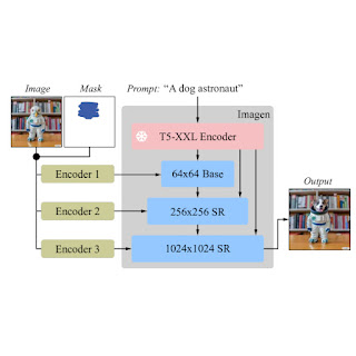
| Given an image, a user-defined mask, and a text prompt, Imagen Editor makes localized edits to the designated areas. The model meaningfully incorporates the user’s intent and performs photorealistic edits. |
Imagen Editor
Imagen Editor is a diffusion-based model fine-tuned on Imagen for editing. It targets improved representations of linguistic inputs, fine-grained control and high-fidelity outputs. Imagen Editor takes three inputs from the user: 1) the image to be edited, 2) a binary mask to specify the edit region, and 3) a text prompt — all three inputs guide the output samples.
Imagen Editor depends on three core techniques for high-quality text-guided image inpainting. First, unlike prior inpainting models (e.g., Palette, Context Attention, Gated Convolution) that apply random box and stroke masks, Imagen Editor employs an object detector masking policy with an object detector module that produces object masks during training. Object masks are based on detected objects rather than random patches and allow for more principled alignment between edit text prompts and masked regions. Empirically, the method helps the model stave off the prevalent issue of the text prompt being ignored when masked regions are small or only partially cover an object (e.g., CogView2).
 |
| Random masks (left) frequently capture background or intersect object boundaries, defining regions that can be plausibly inpainted just from image context alone. Object masks (right) are harder to inpaint from image context alone, encouraging models to rely more on text inputs during training. |
Next, during training and inference, Imagen Editor enhances high resolution editing by conditioning on full resolution (1024×1024 in this work), channel-wise concatenation of the input image and the mask (similar to SR3, Palette, and GLIDE). For the base diffusion 64×64 model and the 64×64→256×256 super-resolution models, we apply a parameterized downsampling convolution (e.g., convolution with a stride), which we empirically find to be critical for high fidelity.
 |
| Imagen is fine-tuned for image editing. All of the diffusion models, i.e., the base model and super-resolution (SR) models, are conditioned on high-resolution 1024×1024 image and mask inputs. To this end, new convolutional image encoders are introduced. |
Finally, at inference we apply classifier-free guidance (CFG) to bias samples to a particular conditioning, in this case, text prompts. CFG interpolates between the text-conditioned and unconditioned model predictions to ensure strong alignment between the generated image and the input text prompt for text-guided image inpainting. We follow Imagen Video and use high guidance weights with guidance oscillation (a guidance schedule that oscillates within a value range of guidance weights). In the base model (the stage-1 64x diffusion), where ensuring strong alignment with text is most critical, we use a guidance weight schedule that oscillates between 1 and 30. We observe that high guidance weights combined with oscillating guidance result in the best trade-off between sample fidelity and text-image alignment.
EditBench
The EditBench dataset for text-guided image inpainting evaluation contains 240 images, with 120 generated and 120 natural images. Generated images are synthesized by Parti and natural images are drawn from the Visual Genome and Open Images datasets. EditBench captures a wide variety of language, image types, and levels of text prompt specificity (i.e., simple, rich, and full captions). Each example consists of (1) a masked input image, (2) an input text prompt, and (3) a high-quality output image used as reference for automatic metrics. To provide insight into the relative strengths and weaknesses of different models, EditBench prompts are designed to test fine-grained details along three categories: (1) attributes (e.g., material, color, shape, size, count); (2) object types (e.g., common, rare, text rendering); and (3) scenes (e.g., indoor, outdoor, realistic, or paintings). To understand how different specifications of prompts affect model performance, we provide three text prompt types: a single-attribute (Mask Simple) or a multi-attribute description of the masked object (Mask Rich) – or an entire image description (Full Image). Mask Rich, especially, probes the models’ ability to handle complex attribute binding and inclusion.
 |
| The full image is used as a reference for successful inpainting. The mask covers the target object with a free-form, non-hinting shape. We evaluate Mask Simple, Mask Rich and Full Image prompts, consistent with conventional text-to-image models. |
Due to the intrinsic weaknesses in existing automatic evaluation metrics (CLIPScore and CLIP-R-Precision) for TGIE, we hold human evaluation as the gold standard for EditBench. In the section below, we demonstrate how EditBench is applied to model evaluation.
Evaluation
We evaluate the Imagen Editor model — with object masking (IM) and with random masking (IM-RM) — against comparable models, Stable Diffusion (SD) and DALL-E 2 (DL2). Imagen Editor outperforms these models by substantial margins across all EditBench evaluation categories.
For Full Image prompts, single-image human evaluation provides binary answers to confirm if the image matches the caption. For Mask Simple prompts, single-image human evaluation confirms if the object and attribute are properly rendered, and bound correctly (e.g., for a red cat, a white cat on a red table would be an incorrect binding). Side-by-side human evaluation uses Mask Rich prompts only for side-by-side comparisons between IM and each of the other three models (IM-RM, DL2, and SD), and indicates which image matches with the caption better for text-image alignment, and which image is most realistic.
 |
| Human evaluation. Full Image prompts elicit annotators’ overall impression of text-image alignment; Mask Simple and Mask Rich check for the correct inclusion of particular attributes, objects and attribute binding. |
For single-image human evaluation, IM receives the highest ratings across-the-board (10–13% higher than the 2nd-highest performing model). For the rest, the performance order is IM-RM > DL2 > SD (with 3–6% difference) except for with Mask Simple, where IM-RM falls 4-8% behind. As relatively more semantic content is involved in Full and Mask Rich, we conjecture IM-RM and IM are benefited by the higher performing T5 XXL text encoder.
 |
| Single-image human evaluations of text-guided image inpainting on EditBench by prompt type. For Mask Simple and Mask Rich prompts, text-image alignment is correct if the edited image accurately includes every attribute and object specified in the prompt, including the correct attribute binding. Note that due to different evaluation designs, Full vs. Mask-only prompts, results are less directly comparable. |
EditBench focuses on fine-grained annotation, so we evaluate models for object and attribute types. For object types, IM leads in all categories, performing 10–11% better than the 2nd-highest performing model in common, rare, and text-rendering.
 |
| Single-image human evaluations on EditBench Mask Simple by object type. As a cohort, models are better at object rendering than text-rendering. |
For attribute types, IM is rated much higher (13–16%) than the 2nd highest performing model, except for in count, where DL2 is merely 1% behind.
 |
| Single-image human evaluations on EditBench Mask Simple by attribute type. Object masking improves adherence to prompt attributes across-the-board (IM vs. IM-RM). |
Side-by-side compared with other models one-vs-one, IM leads in text alignment with a substantial margin, being preferred by annotators compared to SD, DL2, and IM-RM.
 |
| Side-by-side human evaluation of image realism & text-image alignment on EditBench Mask Rich prompts. For text-image alignment, Imagen Editor is preferred in all comparisons. |
Finally, we illustrate a representative side-by-side comparative for all the models. See the paper for more examples.
 |
| Example model outputs for Mask Simple vs. Mask Rich prompts. Object masking improves Imagen Editor’s fine-grained adherence to the prompt compared to the same model trained with random masking. |
Conclusion
We presented Imagen Editor and EditBench, making significant advancements in text-guided image inpainting and the evaluation thereof. Imagen Editor is a text-guided image inpainting fine-tuned from Imagen. EditBench is a comprehensive systematic benchmark for text-guided image inpainting, evaluating performance across multiple dimensions: attributes, objects, and scenes. Note that due to concerns in relation to responsible AI, we are not releasing Imagen Editor to the public. EditBench on the other hand is released in full for the benefit of the research community.
Acknowledgments
Thanks to Gunjan Baid, Nicole Brichtova, Sara Mahdavi, Kathy Meier-Hellstern, Zarana Parekh, Anusha Ramesh, Tris Warkentin, Austin Waters, and Vijay Vasudevan for their generous support. We give thanks to Igor Karpov, Isabel Kraus-Liang, Raghava Ram Pamidigantam, Mahesh Maddinala, and all the anonymous human annotators for their coordination to complete the human evaluation tasks. We are grateful to Huiwen Chang, Austin Tarango, and Douglas Eck for providing paper feedback. Thanks to Erica Moreira and Victor Gomes for help with resource coordination. Finally, thanks to the authors of DALL-E 2 for giving us permission to use their model outputs for research purposes.

Fast-track graph ML with GraphStorm: A new way to solve problems on enterprise-scale graphs
We are excited to announce the open-source release of GraphStorm 0.1, a low-code enterprise graph machine learning (ML) framework to build, train, and deploy graph ML solutions on complex enterprise-scale graphs in days instead of months. With GraphStorm, you can build solutions that directly take into account the structure of relationships or interactions between billions of entities, which are inherently embedded in most real-world data, including fraud detection scenarios, recommendations, community detection, and search/retrieval problems.
Until now, it has been notoriously hard to build, train, and deploy graph ML solutions for complex enterprise graphs that easily have billions of nodes, hundreds of billions of edges, and dozens of attributes—just think about a graph capturing Amazon.com products, product attributes, customers, and more. With GraphStorm, we release the tools that Amazon uses internally to bring large-scale graph ML solutions to production. GraphStorm doesn’t require you to be an expert in graph ML and is available under the Apache v2.0 license on GitHub. To learn more about GraphStorm, visit the GitHub repository.
In this post, we provide an introduction to GraphStorm, its architecture, and an example use case of how to use it.
Introducing GraphStorm
Graph algorithms and graph ML are emerging as state-of-the-art solutions for many important business problems like predicting transaction risks, anticipating customer preferences, detecting intrusions, optimizing supply chains, social network analysis, and traffic prediction. For example, Amazon GuardDuty, the native AWS threat detection service, uses a graph with billions of edges to improve the coverage and accuracy of its threat intelligence. This allows GuardDuty to categorize previously unseen domains as highly likely to be malicious or benign based on their association to known malicious domains. By using Graph Neural Networks (GNNs), GuardDuty is able to enhance its capability to alert customers.
However, developing, launching, and operating graph ML solutions takes months and requires graph ML expertise. As a first step, a graph ML scientist has to build a graph ML model for a given use case using a framework like the Deep Graph Library (DGL). Training such models is challenging due to the size and complexity of graphs in enterprise applications, which routinely reach billions of nodes, hundreds of billions of edges, different node and edge types, and hundreds of node and edge attributes. Enterprise graphs can require terabytes of memory storage, requiring graph ML scientists to build complex training pipelines. Finally, after a model has been trained, they have to be deployed for inference, which requires inference pipelines that are just as difficult to build as the training pipelines.
GraphStorm 0.1 is a low-code enterprise graph ML framework that allows ML practitioners to easily pick predefined graph ML models that have been proven to be effective, run distributed training on graphs with billions of nodes, and deploy the models into production. GraphStorm offers a collection of built-in graph ML models, such as Relational Graph Convolutional Networks (RGCN), Relational Graph Attention Networks (RGAT), and Heterogeneous Graph Transformer (HGT) for enterprise applications with heterogeneous graphs, which allow ML engineers with little graph ML expertise to try out different model solutions for their task and select the right one quickly. End-to-end distributed training and inference pipelines, which scale to billion-scale enterprise graphs, make it easy to train, deploy, and run inference. If you are new to GraphStorm or graph ML in general, you will benefit from the pre-defined models and pipelines. If you are an expert, you have all options to tune the training pipeline and model architecture to get the best performance. GraphStorm is built on top of the DGL, a widely popular framework for developing GNN models, and available as open-source code under the Apache v2.0 license.
“GraphStorm is designed to help customers experiment and operationalize graph ML methods for industry applications to accelerate the adoption of graph ML,” says George Karypis, Senior Principal Scientist in Amazon AI/ML research. “Since its release inside Amazon, GraphStorm has reduced the effort to build graph ML-based solutions by up to five times.”
“GraphStorm enables our team to train GNN embedding in a self-supervised manner on a graph with 288 million nodes and 2 billion edges,” Says Haining Yu, Principal Applied Scientist at Amazon Measurement, Ad Tech, and Data Science. “The pre-trained GNN embeddings show a 24% improvement on a shopper activity prediction task over a state-of-the-art BERT- based baseline; it also exceeds benchmark performance in other ads applications.”
“Before GraphStorm, customers could only scale vertically to handle graphs of 500 million edges,” says Brad Bebee, GM for Amazon Neptune and Amazon Timestream. “GraphStorm enables customers to scale GNN model training on massive Amazon Neptune graphs with tens of billions of edges.”
GraphStorm technical architecture
The following figure shows the technical architecture of GraphStorm.

GraphStorm is built on top of PyTorch and can run on a single GPU, multiple GPUs, and multiple GPU machines. It consists of three layers (marked in the yellow boxes in the preceding figure):
- Bottom layer (Dist GraphEngine) – The bottom layer provides the basic components to enable distributed graph ML, including distributed graphs, distributed tensors, distributed embeddings, and distributed samplers. GraphStorm provides efficient implementations of these components to scale graph ML training to billion-node graphs.
- Middle layer (GS training/inference pipeline) – The middle layer provides trainers, evaluators, and predictors to simplify model training and inference for both built-in models and your custom models. Basically, by using the API of this layer, you can focus on the model development without worrying about how to scale the model training.
- Top layer (GS general model zoo) – The top layer is a model zoo with popular GNN and non-GNN models for different graph types. As of this writing, it provides RGCN, RGAT, and HGT for heterogeneous graphs and BERTGNN for textual graphs. In the future, we will add support for temporal graph models such as TGAT for temporal graphs as well as TransE and DistMult for knowledge graphs.
How to use GraphStorm
After installing GraphStorm, you only need three steps to build and train GML models for your application.
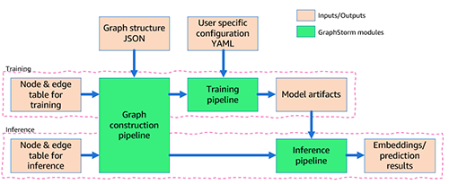
First, you preprocess your data (potentially including your custom feature engineering) and transform it into a table format required by GraphStorm. For each node type, you define a table that lists all nodes of that type and their features, providing a unique ID for each node. For each edge type, you similarly define a table in which each row contains the source and destination node IDs for an edge of that type (for more information, see Use Your Own Data Tutorial). In addition, you provide a JSON file that describes the overall graph structure.
Second, via the command line interface (CLI), you use GraphStorm’s built-in construct_graph component for some GraphStorm-specific data processing, which enables efficient distributed training and inference.
Third, you configure the model and training in a YAML file (example) and, again using the CLI, invoke one of the five built-in components (gs_node_classification, gs_node_regression, gs_edge_classification, gs_edge_regression, gs_link_prediction) as training pipelines to train the model. This step results in the trained model artifacts. To do inference, you need to repeat the first two steps to transform the inference data into a graph using the same GraphStorm component (construct_graph) as before.
Finally, you can invoke one of the five built-in components, the same that was used for model training, as an inference pipeline to generate embeddings or prediction results.
The overall flow is also depicted in the following figure.
In the following section, we provide an example use case.
Make predictions on raw OAG data
For this post, we demonstrate how easily GraphStorm can enable graph ML training and inference on a large raw dataset. The Open Academic Graph (OAG) contains five entities (papers, authors, venues, affiliations, and field of study). The raw dataset is stored in JSON files with over 500 GB.
Our task is to build a model to predict the field of study of a paper. To predict the field of study, you can formulate it as a multi-label classification task, but it’s difficult to use one-hot encoding to store the labels because there are hundreds of thousands of fields. Therefore, you should create field of study nodes and formulate this problem as a link prediction task, predicting which field of study nodes a paper node should connect to.
To model this dataset with a graph method, the first step is to process the dataset and extract entities and edges. You can extract five types of edges from the JSON files to define a graph, shown in the following figure. You can use the Jupyter notebook in the GraphStorm example code to process the dataset and generate five entity tables for each entity type and five edge tables for each edge type. The Jupyter notebook also generates BERT embeddings on the entities with text data, such as papers.

After defining the entities and edges between the entities, you can create mag_bert.json, which defines the graph schema, and invoke the built-in graph construction pipeline construct_graph in GraphStorm to build the graph (see the following code). Even though the GraphStorm graph construction pipeline runs in a single machine, it supports multi-processing to process nodes and edge features in parallel (--num_processes) and can store entity and edge features on external memory (--ext-mem-workspace) to scale to large datasets.
To process such a large graph, you need a large-memory CPU instance to construct the graph. You can use an Amazon Elastic Compute Cloud (Amazon EC2) r6id.32xlarge instance (128 vCPU and 1 TB RAM) or r6a.48xlarge instances (192 vCPU and 1.5 TB RAM) to construct the OAG graph.
After constructing a graph, you can use gs_link_prediction to train a link prediction model on four g5.48xlarge instances. When using the built-in models, you only invoke one command line to launch the distributed training job. See the following code:
After the model training, the model artifact is saved in the folder /data/mag_lp_model.
Now you can run link prediction inference to generate GNN embeddings and evaluate the model performance. GraphStorm provides multiple built-in evaluation metrics to evaluate model performance. For link prediction problems, for example, GraphStorm automatically outputs the metric mean reciprocal rank (MRR). MRR is a valuable metric for evaluating graph link prediction models because it assesses how high the actual links are ranked among the predicted links. This captures the quality of predictions, making sure our model correctly prioritizes true connections, which is our objective here.
You can run inference with one command line, as shown in the following code. In this case, the model reaches an MRR of 0.31 on the test set of the constructed graph.
Note that the inference pipeline generates embeddings from the link prediction model. To solve the problem of finding the field of study for any given paper, simply perform a k-nearest neighbor search on the embeddings.
Conclusion
GraphStorm is a new graph ML framework that makes it easy to build, train, and deploy graph ML models on industry graphs. It addresses some key challenges in graph ML, including scalability and usability. It provides built-in components to process billion-scale graphs from raw input data to model training and model inference and has enabled multiple Amazon teams to train state-of-the-art graph ML models in various applications. Check out our GitHub repository for more information.
About the Authors
 Da Zheng is a senior applied scientist at AWS AI/ML research leading a graph machine learning team to develop techniques and frameworks to put graph machine learning in production. Da got his PhD in computer science from the Johns Hopkins University.
 Florian Saupe is a Principal Technical Product Manager at AWS AI/ML research supporting advanced science teams like the graph machine learning group and improving products like Amazon DataZone with ML capabilities. Before joining AWS, Florian lead technical product management for automated driving at Bosch, was a strategy consultant at McKinsey & Company, and worked as a control systems/robotics scientist – a field in which he holds a phd.
Eye in the Sky With AI: UCSB Initiative Aims to Pulverize Space Threats Using NVIDIA RTX
When meteor showers occur every few months, viewers get to watch a dazzling scene of shooting stars and light streaks scattering across the night sky.
Normally, meteors are just small pieces of rock and dust from space that quickly burn up upon entering Earth’s atmosphere. But the story would take a darker turn if a comet or asteroid is a little too large and heading directly toward Earth’s surface with minimal warning time.
Such a scenario is what physics professor Philip Lubin and some of his undergraduates at the University of California, Santa Barbara, are striving to counteract.
The team recently received phase II funding from NASA to explore a new, more practical approach to planetary defense — one that would allow them to detect and mitigate any threats much faster and more efficiently. Their initiative is called PI-Terminal Planetary Defense, with the PI standing for “Pulverize It.”
To help the team train and speed up the AI and machine learning algorithms they’re developing to detect threats that are on a collision course with Earth, NVIDIA, as part of its Applied Research Accelerator Program, has given the group an NVIDIA RTX A6000 graphics card.
Taking AI to the Sky
Every day, approximately 100 tons of small debris rain down on Earth, but they quickly disintegrate in the atmosphere with very few surviving to reach the surface. Larger asteroids, however, like those responsible for the craters visible on the moon’s surface, pose a real danger to life on Earth.
On average, about every 60 years, an asteroid that’s larger than 65 feet in diameter will appear, similar to the one that exploded over Chelyabinsk, Russia, in 2013, with the energy equivalent of about 440,000 tons of TNT, according to NASA.
The PI-Terminal Planetary Defense initiative aims to detect relevant threats sooner, and then use an array of hypervelocity kinetic penetrators to pulverize and disassemble an asteroid or small comet to greatly minimize the threat.
The traditional approach for planetary defense has involved deflecting threats, but Pulverize-It turns to effectively breaking up the asteroid or comet into much smaller fragments, which then burn up in the Earth’s atmosphere at high altitudes, causing little ground damage. This allows much more rapid mitigation.
Recognizing threats is the first critical step — this is where Lubin and his students tapped into the power of AI.
Many modern surveys collect massive amounts of astrophysical data, but the speed of data collection is faster than the ability to process and analyze the collected images. Lubin’s group is designing a much larger survey specifically for planetary defense that would generate even larger amounts of data that need to be rapidly processed.
Through machine learning, the group trained a neural network called You Only Look Once Darknet. It’s a near real-time object detection system that operates in less than 25 milliseconds per image. The group used a large dataset of labeled images to pretrain the neural network, allowing the model to extract low-level, geometric features like lines, edges and circles, and in and in particular threats such as asteroids and comets.
Early results showed that the source extraction through machine learning was up to 10x faster and nearly 3x more accurate than traditional methods.
Lubin and his group accelerated their image analysis process by approximately 100x, with the help of the NVIDIA RTX A6000 GPU, as well as the CUDA parallel computing platform and programming model.
“Initially, our pipeline — which aims for real-time image processing — took 10 seconds for our subtraction step,” said Lubin. “By implementing the NVIDIA RTX A6000, we immediately cut this processing time to 0.15 seconds.”
Combining this new computational power with the expanded 48GB of VRAM enabled the team to implement new CuPy-based algorithms, which greatly reduced their subtraction and identification time, allowing the entire pipeline to run in just six seconds.
NVIDIA RTX Brings Meteor Memory
One of the group’s biggest technical challenges has been meeting the GPU memory requirement, as well as decreasing the run-time of the training processes. As the project grows, Lubin and his students accumulate increasingly large amounts of data for training. But as the datasets expanded, they needed a GPU that could handle the massive file sizes.
The RTX A6000’s 48GB of memory allows teams to handle the most complex graphics and datasets without worrying about hindering performance.
“Each image will be about 100 megapixels, and we’re putting many images inside the memory of the RTX GPU,” said Lubin. “It helps mitigate the bottleneck of getting data in and out.”
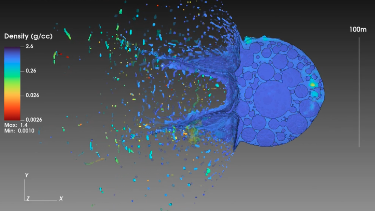
The group works on simulations that demonstrate various phases from the project, including the ground effects from shock waves, as well as the optical light pulses from each fragment that burns in the Earth’s atmosphere. These simulations are done locally, running on custom-developed codes written in multithreaded, multiprocessor C++ and Python.
The image processing pipeline for rapid threat detection runs on custom C++, Python and CUDA codes using multiple Intel Xeon processors and the NVIDIA RTX A6000 GPU.
Other simulations, like one that features the hypervelocity intercept of the threat fragments, are accomplished using the NASA Advanced Supercomputing (NAS) facility at the NASA Ames Research Center. The facility is constantly upgraded and offers over 13 petaflops of computing performance. These visualizations run on the NAS supercomputers equipped with Intel Xeon CPUs and NVIDIA RTX A6000 GPUs.
Check out some of these simulations on the UCSB Group’s Deepspace YouTube channel.
Learn more about the PI-Terminal Planetary Defense project and NVIDIA RTX.
More-inclusive speech recognition with cross-utterance rescoring
In a top-3% paper at ICASSP, Amazon researchers adapt graph-based label propagation to improve speech recognition on underrepresented pronunciations.Read More