This research paper was accepted by the 50th EATCS International Colloquium on Automata, Languages and Programming (ICALP 2023), which is dedicated to advancing the field of theoretical computer science.

In the rapidly evolving landscape of cloud computing, escalating demand for cloud resources is placing immense pressure on cloud providers, driving them to consistently invest in new hardware to accommodate datacenters’ expanding capacity needs. Consequently, the ability to power all this hardware has emerged as a key bottleneck, as devices that power datacenters have limited capacity and necessitate efficient utilization. Efficiency is crucial, not only to lower operational costs and subsequently prices to consumers, but also to support the sustainable use of resources, ensure their long-term availability, and preserve the environment for future generations.
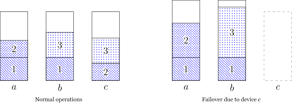
At the same time, it is of the utmost importance to ensure power availability for servers, particularly in the event of a power device failure. Modern datacenter architectures have adopted a strategy to mitigate this risk by avoiding the reliance on a single power source for each server. Instead, each server is powered by two devices. Under normal operations, a server draws half its required power from each device. In the event of a failover, the remaining device steps in to support the server’s full power demand, potentially operating at an increased capacity during the failover period.
Spotlight: On-Demand EVENT

Microsoft Research Summit 2022
On-Demand
Watch now to learn about some of the most pressing questions facing our research community and listen in on conversations with 120+ researchers around how to ensure new technologies have the broadest possible benefit for humanity.
Challenges of optimizing power allocation
In our paper, “Online Demand Scheduling with Failovers,” which we’re presenting at the 50th EATCS International Colloquium on Automata, Languages and Programming, (ICALP 2023), we explore a simplified model that emphasizes power management to determine how to optimally place servers within a datacenter. Our model contains multiple power devices and new servers (demands), where each power device has a normal capacity of 1 and a larger failover capacity, B. Demands arrive over time, each with a power requirement, and we must irrevocably assign each demand to a pair of power devices with sufficient capacity. The goal is to maximize the total power of the assigned demands until we are forced to reject a demand due to lack of power. This helps us maximize the usage of the available power devices.
One crucial aspect of this model is the presence of uncertainty. We assign capacity for each demand without knowing future needs. This uncertainty adds complexity, as selection of device pairs for each demand must be carefully executed to avoid allocations that could hinder the placement of future demands. Figure 2 provides an illustration.
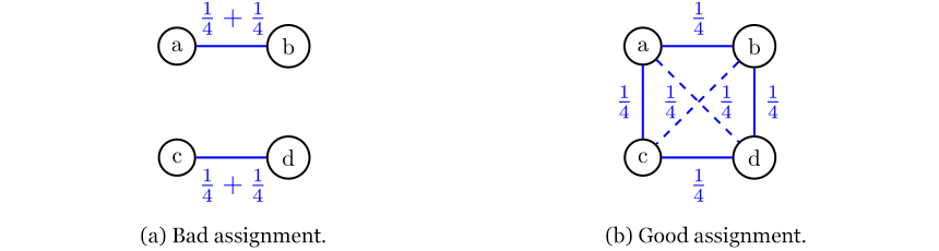
The example in Figure 2 suggests that we should spread the demands across device pairs. Otherwise, pairs with large loads could have a big impact on the remaining devices should one device fail. On the other hand, there is a danger in spreading out the demands too much and not leaving enough devices free, as shown in Figure 3.
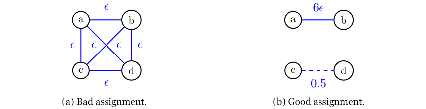
In analyzing the examples in Figures 2 and 3, it becomes clear that striking the right balance is crucial. This entails effectively distributing demands across pairs to minimize any consequences resulting from failovers while also ensuring the availability of an adequate number of devices to meet future demand. Attaining the optimal allocation avoids prematurely ending up with an unassignable demand.
To tackle this challenge, we developed algorithms that are guaranteed to efficiently utilize the available power resources. In fact, our allocations are provably close to optimal, even without upfront knowledge of the demands. Our algorithms essentially conquer the inherent uncertainty of the problem.
Optimizing for the worst-case scenario
Our first algorithm takes a conservative approach, protecting against the worst-case scenario. It guarantees that, regardless of the sequence of demand requests, it will utilize at least half of the power when compared with an optimal solution that has prior knowledge of all demands. As we show in the paper, this result represents the optimal outcome achievable in the most challenging instances.
To effectively strike a balance between distributing demands across devices and ensuring sufficient device availability, the goal of this algorithm is to group demands based on their power requirements. Each group of demands is then allocated separately to an appropriately sized collection of devices. The algorithm aims to consolidate similar demands in controlled regions, enabling efficient utilization of failover resources. Notably, we assign at most one demand per pair of devices in each collection, except in the case of minor demands, which are handled separately.
Optimizing for real-world demand
Because the previous algorithm prioritizes robustness against the worst-case demand sequences, it may unintentionally result in underutilizing the available power by a factor of ½, which is unavoidable in that setting. However, these worst-case scenarios are uncommon in typical datacenter operations. Accordingly, we shifted our focus to a more realistic model where demands arise from an unknown probability distribution. We designed our second algorithm in this stochastic arrival model, demonstrating that as the number of demands and power devices increases, its assignment progressively converges to the optimal omniscient solution, ensuring that no power is wasted.
To achieve this, the algorithm learns from historical data, enabling informed assignment decisions based on past demands. By creating “allocation templates” derived from previous demands, we learn how to allocate future demands. To implement this concept and prove its guarantee, we have developed new tools in probability and optimization that may be valuable in addressing similar problems in the future.
The post Microsoft at ICALP 2023: Deploying cloud capacity robustly against power failures appeared first on Microsoft Research.