Familiar topics such as question answering and natural-language understanding remain well represented, but a new concentration on language modeling and multimodal models reflect the spread of generative AI.Read More
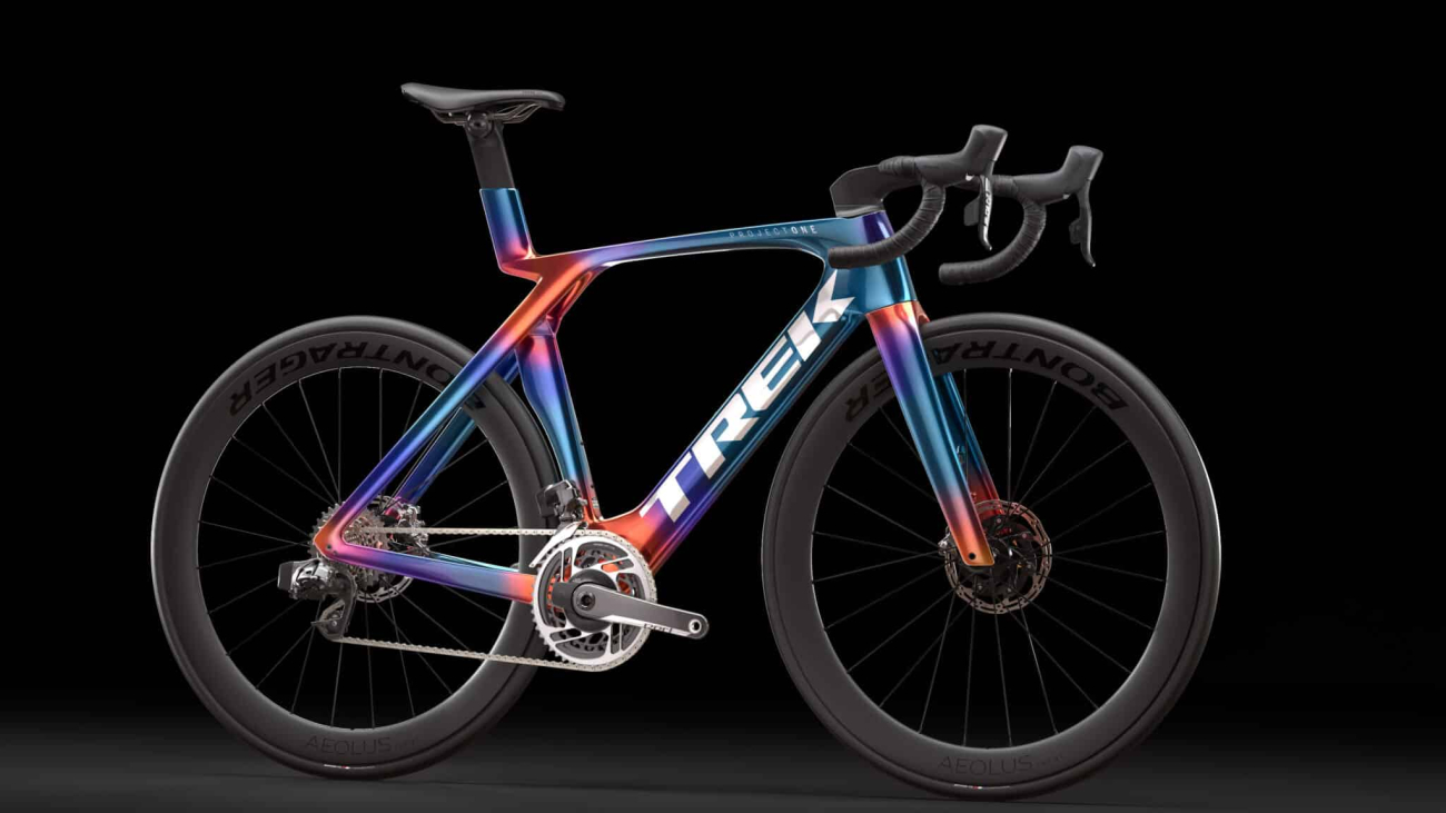
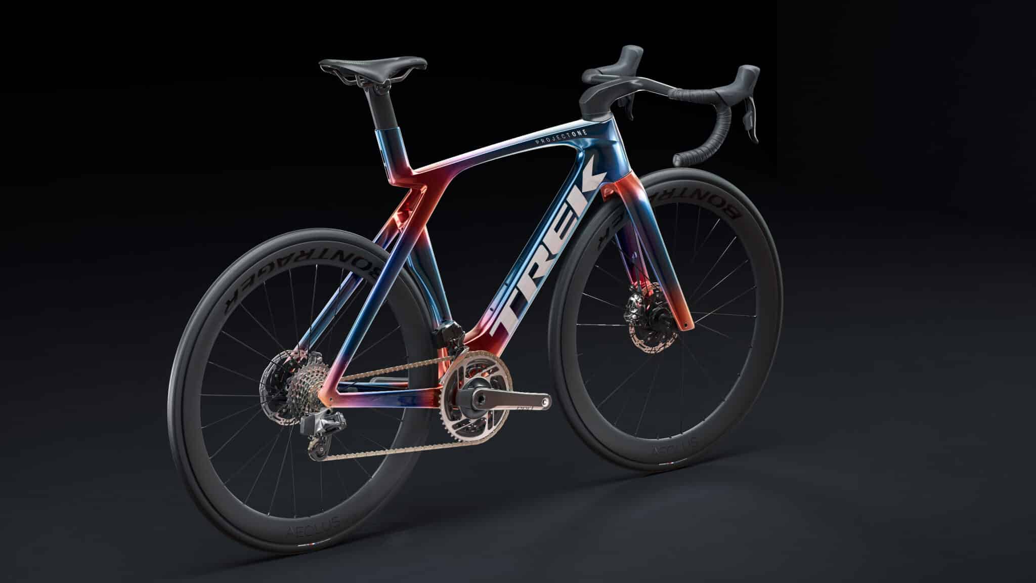
Design Speed Takes the Lead: Trek Bicycle Competes in Tour de France With Bikes Developed Using NVIDIA GPUs
NVIDIA RTX is spinning new cycles for designs. Trek Bicycle is using GPUs to bring design concepts to life.
The Wisconsin-based company, one of the largest bicycle manufacturers in the world, aims to create bikes with the highest-quality craftsmanship. With its new partner Lidl, an international retailer chain, Trek Bicycle also owns a cycling team, now called Lidl-Trek. The team is competing in the annual Tour de France stage race on Trek Bicycle’s flagship lineup, which includes the Emonda, Madone and Speed Concept. Many of the team’s accessories and equipment, such as the wheels and road race helmets, were also designed at Trek.
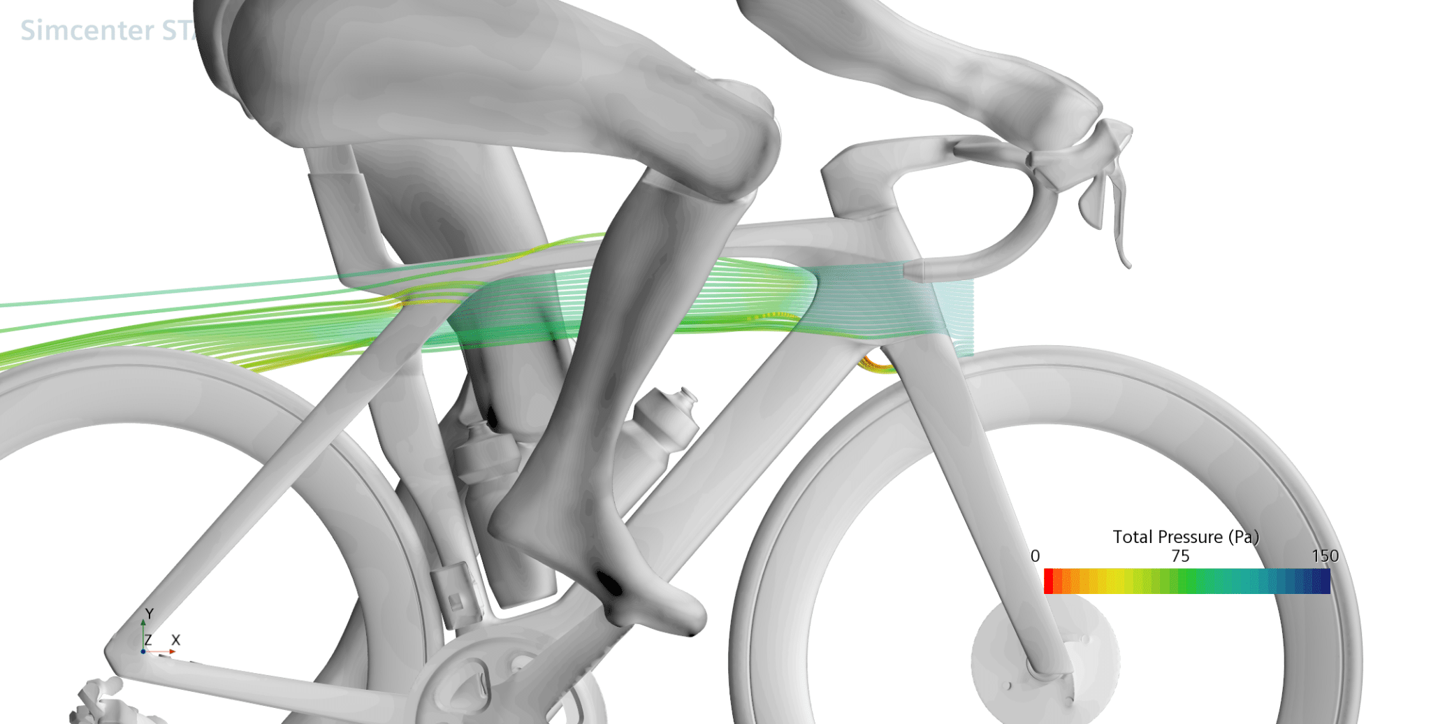
Bicycle design involves complex physics — and a key challenge is balancing aerodynamic efficiency with comfort and ride quality. To address this, the team at Trek is using NVIDIA A100 Tensor Core GPUs to run high-fidelity computational fluid dynamics (CFD) simulations, setting new benchmarks for aerodynamics in a bicycle that’s also comfortable to ride and handles smoothly.
The designers and engineers are further enhancing their workflows using NVIDIA RTX technology in Dell Precision workstations, including the NVIDIA RTX A5500 GPU, as well as a Dell Precision 7920 running dual RTX A6000 GPUs.
Visualizing Bicycle Designs in Real Time
To kick off the product design process, the team starts with user research to generate early design concepts and develop a range of ideas. Then, they build prototypes and iterate the design as needed.
To improve performance, the bikes need to feel a certain way, whether riders are taking it on the road or the trail. So Trek spends a lot of time with athletes to figure out where to make critical changes, including tweaks to geometry and the flexibility of the frame and taking the edge off of bumps.
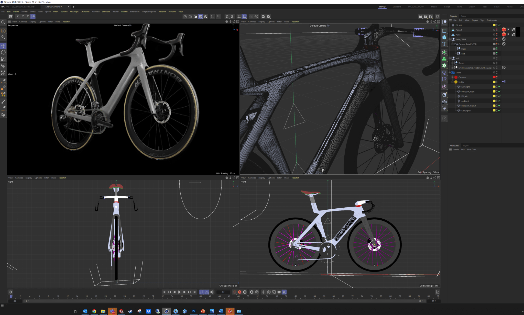
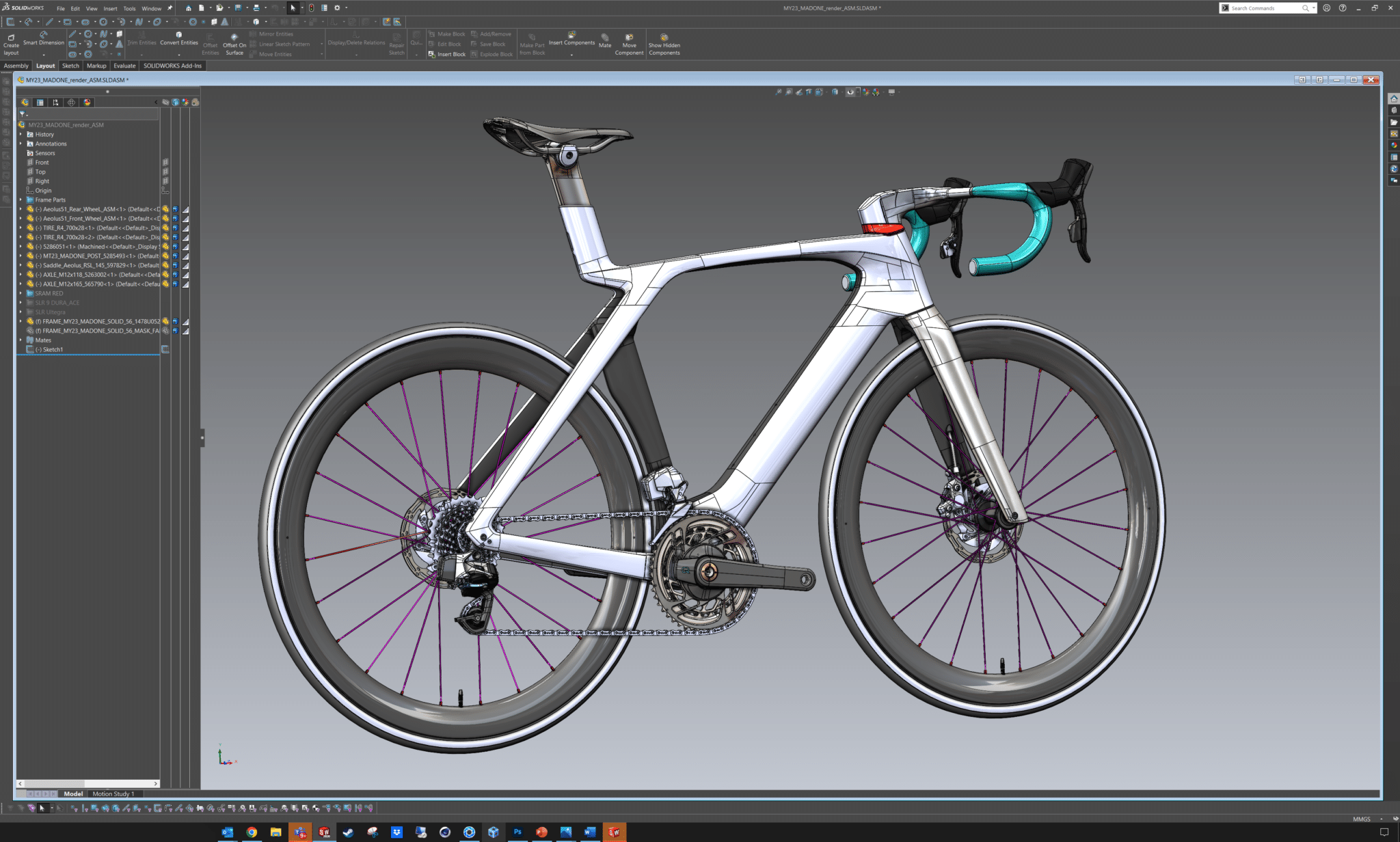
The designers use graphics-intensive applications tools for their computer-aided design workflows, including Adobe Substance 3D, Cinema 4D, KeyShot, Redshift and SOLIDWORKS. For CFD simulations, the Trek Performance Research team uses Simcenter STAR-CCM+ from Siemens Digital Industries Software to take advantage of the GPU processing capabilities.
NVIDIA RTX GPUs provided Trek with a giant leap forward for design and engineering. The visualization team can easily tap into RTX technology to iterate quicker and show more options in designs. They can also use Cinema 4D and Redshift with RTX to produce high-quality renderings and even to visualize different designs in near real time.
Michael Hammond, the lead for digital visual communications at Trek Bicycle, explains the importance of having time for iterations. “The faster we can render an image or animation, the faster we can improve it,” he said. “But at the same time, we don’t want to lose details or spend time recreating models.”
With the help of the RTX A5500, Trek’s digital visual team can push past creative limits and reach the final design much faster. “On average, the RTX GPU performs 12x faster than our network rendering, which is on CPU cores,” said Hammond. “For a render that takes about two hours to complete on our network, it only takes around 10-12 minutes on the RTX A5500 — that means I can do 12x the iterations, which leads to better quality rendering and animation in less time.”
Accelerating CFD Simulations
Over the past decade, adoption of CFD has grown as a critical tool for engineers and equipment designers because it allows them to gain better insights into the behavior of their designs. But CFD is more than an analysis tool — it’s used to make improvements without having to resort to time-consuming and expensive physical testing for every design. This is why Trek has integrated CFD into its product development workflows.
The aerodynamics team at Trek relies on Simcenter STAR-CCM+ to optimize the performance of each bike. To provide a comfortable ride and smooth handling while achieving the best aerodynamic performance, the Trek engineers designed the latest generation Madone to use IsoFlow, a unique feature designed to increase rider comfort while reducing drag.
The Simcenter STAR-CCM+ simulations benefit from the speed of accelerated GPU computing, and it enabled the engineers to cut down simulation runtimes by 85 days, as they could run CFD simulations 4-5x faster on NVIDIA A100 GPUs compared to their 128-core CPU-based HPC server.
The team can also analyze more complex physics in CFD to better understand how the air is moving in real-world unsteady conditions.
“Now that we can run higher fidelity and more accurate simulations and still meet deadlines, we are able to reduce wind tunnel testing time for significant cost savings,” said John Davis, the aerodynamics lead at Trek Bicycle. “Within the first two months of running CFD on our GPUs, we were able to cancel a planned wind tunnel test due to the increased confidence we had in simulation results.”
Learn more about Trek Bicycle and GPU-accelerated Simcenter STAR-CCM+.
And join us at SIGGRAPH, which runs from Aug. 6-10, to see the latest technologies shaping the future of design and simulation.
Renovating computer systems securely and progressively with APRON
This research paper was accepted by 2023 USENIX Annual Technical Conference (ATC), which is dedicated to advancing the field of systems research.
Whether they’re personal computers or cloud instances, it’s crucial to ensure that the computer systems people use every day are reliable and secure. The validity of these systems is critical because if storage devices containing important executables and data become invalid, the entire system is affected. Numerous events can jeopardize the validity of computer systems or the data stored in them, such as malicious attacks like ransomware; hardware or software errors can corrupt a system, and a lack of regular maintenance such as patch installations can cause a system to become outdated. While the ideal scenario would be to create a flawless computer system that prevents such invalid states from occurring, achieving this perfection may prove challenging in practice.
Cyber-resilient system and recovery
A cyber-resilient system is a practical approach for addressing invalid system states. This resilient system effectively identifies suspicious state corruption or preservation by analyzing various internal and external signals. If it confirms any corruption, it recovers the system. In our previous work, which we presented at the 40th IEEE Symposium on Security and Privacy, we demonstrated the feasibility of unconditional system recovery using a very small hardware component. This component forcefully resets the entire system, making it execute trusted tiny code for system boot and recovery when no authenticated deferral request is present.
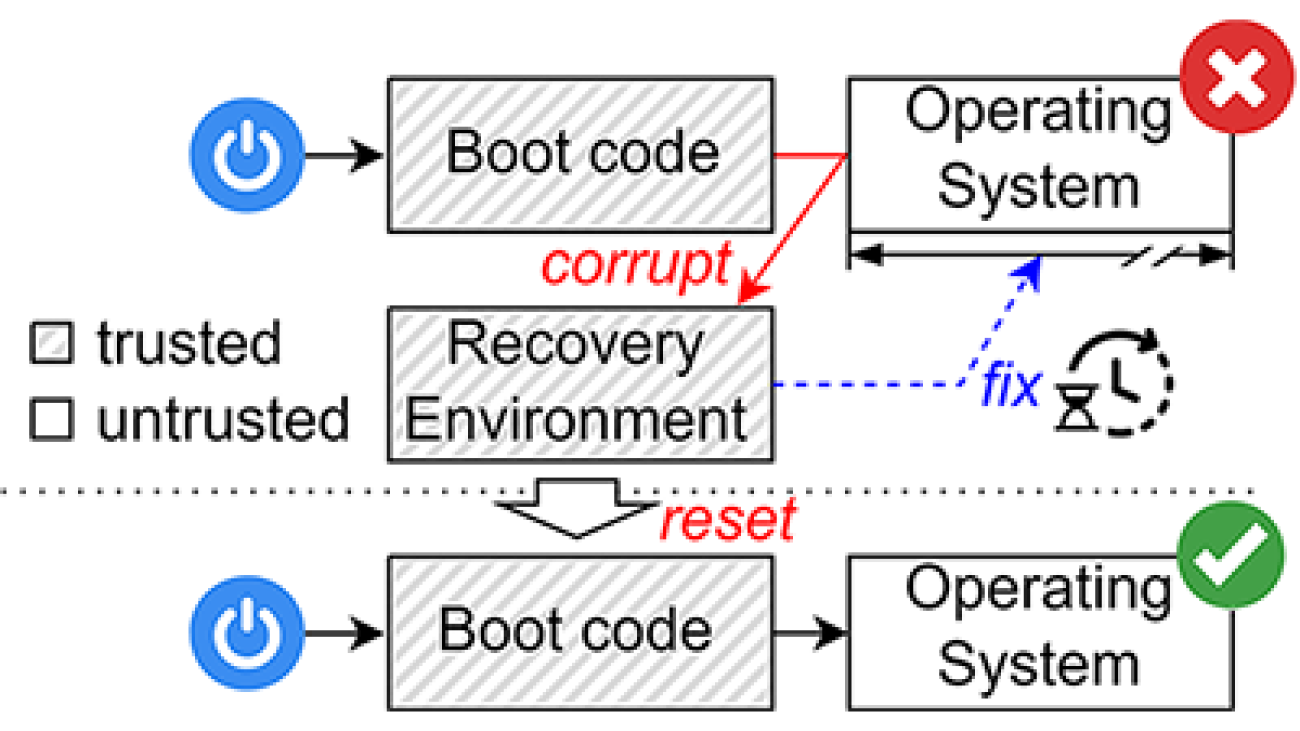
However, existing recovery mechanisms, including our previous work, primarily focus on when to recover a system rather than how. Consequently, these mechanisms overlook the efficiency and security issues that can arise during system recovery. Typically, these mechanisms incorporate a dedicated recovery environment responsible for executing the recovery task. Upon system reset, if the system is found to be invalid, as illustrated in Figure 1, the recovery environment is invoked. In this scenario, the recovery environment fully restores the system using a reference image downloaded from a reliable source or a separate location where it was securely stored.

Unfortunately, performing a full system recovery leads to prolonged system downtime because the recovery environment is incapable of supporting any other regular task expected from a computer system. In other words, the system remains unavailable during the recovery process. Moreover, choosing to download the reference image only serves to extend overall downtime. Although using the stored image slightly relieves this issue, it introduces security concerns, as the stored image might be outdated. One can argue that a full recovery can be circumvented by inspecting each file or data block for validity and selectively recovering only the affected ones. However, this delta recovery approach is lengthier than a full recovery due to the additional calculations required for determining differences and the inefficient utilization of modern, throughput-oriented block storage devices.
Secure and progressive system renovation
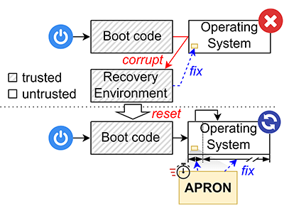
In our paper “APRON: Authenticated and Progressive System Image Renovation,” which we are presenting at the 2023 USENIX Annual Technical Conference (USENIX ATC 2023), we introduce APRON, a novel mechanism for securely renovating a computer system with minimal downtime. APRON differs from conventional recovery mechanisms in a crucial way: it does not fully recover the system within the recovery environment. Instead, it selectively addresses a small set of system components, or data blocks containing them, that are necessary for booting and system recovery, including the operating system kernel and the APRON kernel module, as shown in 2 Once these components are recovered, the system boots into a partially renovated state and can perform regular tasks, progressively recovering other invalid system components as needed.
This design allows APRON to significantly decrease downtime during system recovery by up to 28 times, compared with a normal system recovery, when retrieving portions of the reference image from a remote storage server connected through a 1 Gbps link. In addition, APRON incorporates a background thread dedicated to renovating the remaining invalid system components that might be accessed in the future. This background thread operates with low priority to avoid disrupting important foreground tasks. Throughout both renovation activities, APRON incurs an average runtime overhead of only 9% across a range of real-world applications. Once the renovation process is complete, runtime overhead disappears.
APRON’s differentiator lies in its unique approach: the APRON kernel module acts as an intermediary between application or kernel threads and the system storage device, allowing it to verify and recover each data block on demand, as shown in Figure 3. When a block is requested, APRON follows a straightforward process. If the requested block is valid, APRON promptly delivers it to the requester. If it is found to be invalid, APRON employs a reference image to fix the block before serving it to the requester.
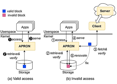
To efficiently and securely verify arbitrary data blocks, APRON uses a Merkle hash tree, which cryptographically summarizes every data block of the reference image. APRON further cryptographically authenticates the Merkle tree’s root hash value so that a malicious actor cannot tamper with it. To further improve performance, APRON treats zero blocks (data blocks filled with zeros) as a special case and performs deduplication to avoid repeatedly retrieving equivalent blocks. We discuss the technical details of this process in our paper.
Looking forward—extending APRON to container engines and hypervisors
APRON’s simple and widely applicable core design can easily apply to other use cases requiring efficient and secure image recovery or provisioning. We are currently exploring the possibility of implementing APRON within a container engine or hypervisor to realize an agentless APRON for container layers or virtual disk images. By extending APRON’s capabilities to these environments, we aim to provide an efficient and reliable image recovery and provisioning process without needing to modify container instances or add a guest operating system.
The post Renovating computer systems securely and progressively with APRON appeared first on Microsoft Research.

Google at ACL 2023
.jpg)
This week, the 61st annual meeting of the Association for Computational Linguistics (ACL), a premier conference covering a broad spectrum of research areas that are concerned with computational approaches to natural language, is taking place online.
As a leader in natural language processing and understanding, and a Diamond Level sponsor of ACL 2023, Google will showcase the latest research in the field with over 50 publications, and active involvement in a variety of workshops and tutorials.
If you’re registered for ACL 2023, we hope that you’ll visit the Google booth to learn more about the projects at Google that go into solving interesting problems for billions of people. You can also learn more about Google’s participation below (Google affiliations in bold).
Board and Organizing Committee
Area chairs include: Dan Garrette
Workshop chairs include: Annie Louis
Publication chairs include: Lei Shu
Program Committee includes: Vinodkumar Prabhakaran, Najoung Kim, Markus Freitag
Spotlight papers
NusaCrowd: Open Source Initiative for Indonesian NLP Resources
Samuel Cahyawijaya, Holy Lovenia, Alham Fikri Aji, Genta Winata, Bryan Wilie, Fajri Koto, Rahmad Mahendra, Christian Wibisono, Ade Romadhony, Karissa Vincentio, Jennifer Santoso, David Moeljadi, Cahya Wirawan, Frederikus Hudi, Muhammad Satrio Wicaksono, Ivan Parmonangan, Ika Alfina, Ilham Firdausi Putra, Samsul Rahmadani, Yulianti Oenang, Ali Septiandri, James Jaya, Kaustubh Dhole, Arie Suryani, Rifki Afina Putri, Dan Su, Keith Stevens, Made Nindyatama Nityasya, Muhammad Adilazuarda, Ryan Hadiwijaya, Ryandito Diandaru, Tiezheng Yu, Vito Ghifari, Wenliang Dai, Yan Xu, Dyah Damapuspita, Haryo Wibowo, Cuk Tho, Ichwanul Karo Karo, Tirana Fatyanosa, Ziwei Ji, Graham Neubig, Timothy Baldwin, Sebastian Ruder, Pascale Fung, Herry Sujaini, Sakriani Sakti, Ayu Purwarianti
Optimizing Test-Time Query Representations for Dense Retrieval
Mujeen Sung, Jungsoo Park, Jaewoo Kang, Danqi Chen, Jinhyuk Lee
PropSegmEnt: A Large-Scale Corpus for Proposition-Level Segmentation and Entailment Recognition
Sihao Chen*, Senaka Buthpitiya, Alex Fabrikant, Dan Roth, Tal Schuster
Distilling Step-by-Step! Outperforming Larger Language Models with Less Training Data and Smaller Model Sizes
Cheng-Yu Hsieh*, Chun-Liang Li, Chih-Kuan Yeh, Hootan Nakhost, Yasuhisa Fujii, Alex Ratner, Ranjay Krishna, Chen-Yu Lee, Tomas Pfister
Large Language Models with Controllable Working Memory
Daliang Li, Ankit Singh Rawat, Manzil Zaheer, Xin Wang, Michal Lukasik, Andreas Veit, Felix Yu, Sanjiv Kumar
OpineSum: Entailment-Based Self-Training for Abstractive Opinion Summarization
Annie Louis, Joshua Maynez
RISE: Leveraging Retrieval Techniques for Summarization Evaluation
David Uthus, Jianmo Ni
Follow the Leader(board) with Confidence: Estimating p-Values from a Single Test Set with Item and Response Variance
Shira Wein*, Christopher Homan, Lora Aroyo, Chris Welty
SamToNe: Improving Contrastive Loss for Dual Encoder Retrieval Models with Same Tower Negatives
Fedor Moiseev, Gustavo Hernandez Abrego, Peter Dornbach, Imed Zitouni, Enrique Alfonseca, Zhe Dong
Papers
Searching for Needles in a Haystack: On the Role of Incidental Bilingualism in PaLM’s Translation Capability
Eleftheria Briakou, Colin Cherry, George Foster
Prompting PaLM for Translation: Assessing Strategies and Performance
David Vilar, Markus Freitag, Colin Cherry, Jiaming Luo, Viresh Ratnakar, George Foster
Query Refinement Prompts for Closed-Book Long-Form QA
Reinald Kim Amplayo, Kellie Webster, Michael Collins, Dipanjan Das, Shashi Narayan
To Adapt or to Annotate: Challenges and Interventions for Domain Adaptation in Open-Domain Question Answering
Dheeru Dua*, Emma Strubell, Sameer Singh, Pat Verga
FRMT: A Benchmark for Few-Shot Region-Aware Machine Translation (see blog post)
Parker Riley, Timothy Dozat, Jan A. Botha, Xavier Garcia, Dan Garrette, Jason Riesa, Orhan Firat, Noah Constant
Conditional Generation with a Question-Answering Blueprint
Shashi Narayan, Joshua Maynez, Reinald Kim Amplayo, Kuzman Ganchev, Annie Louis, Fantine Huot, Anders Sandholm, Dipanjan Das, Mirella Lapata
Coreference Resolution Through a Seq2Seq Transition-Based System
Bernd Bohnet, Chris Alberti, Michael Collins
Cross-Lingual Transfer with Language-Specific Subnetworks for Low-Resource Dependency Parsing
Rochelle Choenni, Dan Garrette, Ekaterina Shutova
DAMP: Doubly Aligned Multilingual Parser for Task-Oriented Dialogue
William Held*, Christopher Hidey, Fei Liu, Eric Zhu, Rahul Goel, Diyi Yang, Rushin Shah
RARR: Researching and Revising What Language Models Say, Using Language Models
Luyu Gao*, Zhuyun Dai, Panupong Pasupat, Anthony Chen*, Arun Tejasvi Chaganty, Yicheng Fan, Vincent Y. Zhao, Ni Lao, Hongrae Lee, Da-Cheng Juan, Kelvin Guu
Benchmarking Large Language Model Capabilities for Conditional Generation
Joshua Maynez, Priyanka Agrawal, Sebastian Gehrmann
Crosslingual Generalization Through Multitask Fine-Tuning
Niklas Muennighoff, Thomas Wang, Lintang Sutawika, Adam Roberts, Stella Biderman, Teven Le Scao, M. Saiful Bari, Sheng Shen, Zheng Xin Yong, Hailey Schoelkopf, Xiangru Tang, Dragomir Radev, Alham Fikri Aji, Khalid Almubarak, Samuel Albanie, Zaid Alyafeai, Albert Webson, Edward Raff, Colin Raffel
DisentQA: Disentangling Parametric and Contextual Knowledge with Counterfactual Question Answering
Ella Neeman, Roee Aharoni, Or Honovich, Leshem Choshen, Idan Szpektor, Omri Abend
Resolving Indirect Referring Expressions for Entity Selection
Mohammad Javad Hosseini, Filip Radlinski, Silvia Pareti, Annie Louis
SeeGULL: A Stereotype Benchmark with Broad Geo-Cultural Coverage Leveraging Generative Models
Akshita Jha*, Aida Mostafazadeh Davani, Chandan K Reddy, Shachi Dave, Vinodkumar Prabhakaran, Sunipa Dev
The Tail Wagging the Dog: Dataset Construction Biases of Social Bias Benchmarks
Nikil Selvam, Sunipa Dev, Daniel Khashabi, Tushar Khot, Kai-Wei Chang
Character-Aware Models Improve Visual Text Rendering
Rosanne Liu, Dan Garrette, Chitwan Saharia, William Chan, Adam Roberts, Sharan Narang, Irina Blok, RJ Mical, Mohammad Norouzi, Noah Constant
Cold-Start Data Selection for Better Few-Shot Language Model Fine-Tuning: A Prompt-Based Uncertainty Propagation Approach
Yue Yu, Rongzhi Zhang, Ran Xu, Jieyu Zhang, Jiaming Shen, Chao Zhang
Covering Uncommon Ground: Gap-Focused Question Generation for Answer Assessment
Roni Rabin, Alexandre Djerbetian, Roee Engelberg, Lidan Hackmon, Gal Elidan, Reut Tsarfaty, Amir Globerson
FormNetV2: Multimodal Graph Contrastive Learning for Form Document Information Extraction
Chen-Yu Lee, Chun-Liang Li, Hao Zhang, Timothy Dozat, Vincent Perot, Guolong Su, Xiang Zhang, Kihyuk Sohn, Nikolay Glushinev, Renshen Wang, Joshua Ainslie, Shangbang Long, Siyang Qin, Yasuhisa Fujii, Nan Hua, Tomas Pfister
Dialect-Robust Evaluation of Generated Text
Jiao Sun*, Thibault Sellam, Elizabeth Clark, Tu Vu*, Timothy Dozat, Dan Garrette, Aditya Siddhant, Jacob Eisenstein, Sebastian Gehrmann
MISGENDERED: Limits of Large Language Models in Understanding Pronouns
Tamanna Hossain, Sunipa Dev, Sameer Singh
LAMBADA: Backward Chaining for Automated Reasoning in Natural Language
Mehran Kazemi, Najoung Kim, Deepti Bhatia, Xin Xu, Deepak Ramachandran
LAIT: Efficient Multi-Segment Encoding in Transformers with Layer-Adjustable Interaction
Jeremiah Milbauer*, Annie Louis, Mohammad Javad Hosseini, Alex Fabrikant, Donald Metzler, Tal Schuster
Modular Visual Question Answering via Code Generation (see blog post)
Sanjay Subramanian, Medhini Narasimhan, Kushal Khangaonkar, Kevin Yang, Arsha Nagrani, Cordelia Schmid, Andy Zeng, Trevor Darrell, Dan Klein
Towards Understanding Chain-of-Thought Prompting: An Empirical Study of What Matters
Boshi Wang, Sewon Min, Xiang Deng, Jiaming Shen, You Wu, Luke Zettlemoyer and Huan Sun
Better Zero-Shot Reasoning with Self-Adaptive Prompting
Xingchen Wan*, Ruoxi Sun, Hanjun Dai, Sercan Ö. Arik, Tomas Pfister
Factually Consistent Summarization via Reinforcement Learning with Textual Entailment Feedback
Paul Roit, Johan Ferret, Lior Shani, Roee Aharoni, Geoffrey Cideron, Robert Dadashi, Matthieu Geist, Sertan Girgin, Léonard Hussenot, Orgad Keller, Nikola Momchev, Sabela Ramos, Piotr Stanczyk, Nino Vieillard, Olivier Bachem, Gal Elidan, Avinatan Hassidim, Olivier Pietquin, Idan Szpektor
Natural Language to Code Generation in Interactive Data Science Notebooks
Pengcheng Yin, Wen-Ding Li, Kefan Xiao, Abhishek Rao, Yeming Wen, Kensen Shi, Joshua Howland, Paige Bailey, Michele Catasta, Henryk Michalewski, Oleksandr Polozov, Charles Sutton
Teaching Small Language Models to Reason
Lucie Charlotte Magister*, Jonathan Mallinson, Jakub Adamek, Eric Malmi, Aliaksei Severyn
Using Domain Knowledge to Guide Dialog Structure Induction via Neural Probabilistic Soft Logic
Connor Pryor*, Quan Yuan, Jeremiah Liu, Mehran Kazemi, Deepak Ramachandran, Tania Bedrax-Weiss, Lise Getoor
A Needle in a Haystack: An Analysis of High-Agreement Workers on MTurk for Summarization
Lining Zhang, Simon Mille, Yufang Hou, Daniel Deutsch, Elizabeth Clark, Yixin Liu, Saad Mahamood, Sebastian Gehrmann, Miruna Clinciu, Khyathi Raghavi Chandu and João Sedoc
Industry Track papers
Federated Learning of Gboard Language Models with Differential Privacy
Zheng Xu, Yanxiang Zhang, Galen Andrew, Christopher Choquette, Peter Kairouz, Brendan McMahan, Jesse Rosenstock, Yuanbo Zhang
KAFA: Rethinking Image Ad Understanding with Knowledge-Augmented Feature Adaptation of Vision-Language Models
Zhiwei Jia*, Pradyumna Narayana, Arjun Akula, Garima Pruthi, Hao Su, Sugato Basu, Varun Jampani
ACL Findings papers
Multilingual Summarization with Factual Consistency Evaluation
Roee Aharoni, Shashi Narayan, Joshua Maynez, Jonathan Herzig, Elizabeth Clark, Mirella Lapata
Parameter-Efficient Fine-Tuning for Robust Continual Multilingual Learning
Kartikeya Badola, Shachi Dave, Partha Talukdar
FiDO: Fusion-in-Decoder Optimized for Stronger Performance and Faster Inference
Michiel de Jong*, Yury Zemlyanskiy, Joshua Ainslie, Nicholas FitzGerald, Sumit Sanghai, Fei Sha, William Cohen
A Simple, Yet Effective Approach to Finding Biases in Code Generation
Spyridon Mouselinos, Mateusz Malinowski, Henryk Michalewski
Challenging BIG-Bench Tasks and Whether Chain-of-Thought Can Solve Them
Mirac Suzgun, Nathan Scales, Nathanael Scharli, Sebastian Gehrmann, Yi Tay, Hyung Won Chung, Aakanksha Chowdhery, Quoc Le, Ed Chi, Denny Zhou, Jason Wei
QueryForm: A Simple Zero-Shot Form Entity Query Framework
Zifeng Wang*, Zizhao Zhang, Jacob Devlin, Chen-Yu Lee, Guolong Su, Hao Zhang, Jennifer Dy, Vincent Perot, Tomas Pfister
ReGen: Zero-Shot Text Classification via Training Data Generation with Progressive Dense Retrieval
Yue Yu, Yuchen Zhuang, Rongzhi Zhang, Yu Meng, Jiaming Shen, Chao Zhang
Multilingual Sequence-to-Sequence Models for Hebrew NLP
Matan Eyal, Hila Noga, Roee Aharoni, Idan Szpektor, Reut Tsarfaty
Triggering Multi-Hop Reasoning for Question Answering in Language Models Using Soft Prompts and Random Walks
Kanishka Misra*, Cicero Nogueira dos Santos, Siamak Shakeri
Tutorials
Complex Reasoning in Natural Language
Wenting Zhao, Mor Geva, Bill Yuchen Lin, Michihiro Yasunaga, Aman Madaan, Tao Yu
Generating Text from Language Models
Afra Amini, Ryan Cotterell, John Hewitt, Clara Meister, Tiago Pimentel
Workshops
Simple and Efficient Natural Language Processing (SustaiNLP)
Organizers include: Tal Schuster
Workshop on Online Abuse and Harms (WOAH)
Organizers include: Aida Mostafazadeh Davani
Document-Grounded Dialogue and Conversational Question Answering (DialDoc)
Organizers include: Roee Aharoni
NLP for Conversational AI
Organizers include: Abhinav Rastogi
Computation and Written Language (CAWL)
Organizers include: Kyle Gorman, Brian Roark, Richard Sproat
Computational Morphology and Phonology (SIGMORPHON)
Speakers include: Kyle Gorman
Workshop on Narrative Understanding (WNU)
Organizers include: Elizabeth Clark
* Work done while at Google

On the Stepwise Nature of Self-Supervised Learning
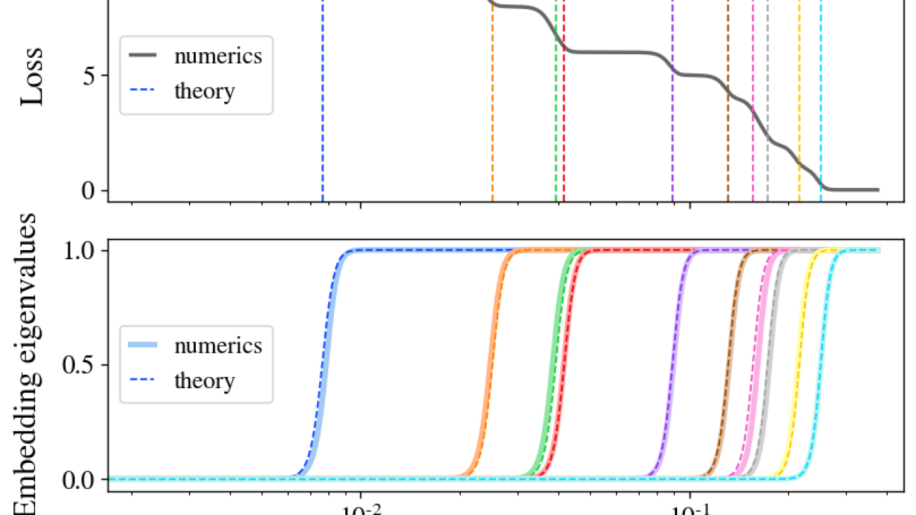
Figure 1: stepwise behavior in self-supervised learning. When training common SSL algorithms, we find that the loss descends in a stepwise fashion (top left) and the learned embeddings iteratively increase in dimensionality (bottom left). Direct visualization of embeddings (right; top three PCA directions shown) confirms that embeddings are initially collapsed to a point, which then expands to a 1D manifold, a 2D manifold, and beyond concurrently with steps in the loss.
It is widely believed that deep learning’s stunning success is due in part to its ability to discover and extract useful representations of complex data. Self-supervised learning (SSL) has emerged as a leading framework for learning these representations for images directly from unlabeled data, similar to how LLMs learn representations for language directly from web-scraped text. Yet despite SSL’s key role in state-of-the-art models such as CLIP and MidJourney, fundamental questions like “what are self-supervised image systems really learning?” and “how does that learning actually occur?” lack basic answers.
Our recent paper (to appear at ICML 2023) presents what we suggest is the first compelling mathematical picture of the training process of large-scale SSL methods. Our simplified theoretical model, which we solve exactly, learns aspects of the data in a series of discrete, well-separated steps. We then demonstrate that this behavior can be observed in the wild across many current state-of-the-art systems.
This discovery opens new avenues for improving SSL methods, and enables a whole range of new scientific questions that, when answered, will provide a powerful lens for understanding some of today’s most important deep learning systems.
On the Stepwise Nature of Self-Supervised Learning
Figure 1: stepwise behavior in self-supervised learning. When training common SSL algorithms, we find that the loss descends in a stepwise fashion (top left) and the learned embeddings iteratively increase in dimensionality (bottom left). Direct visualization of embeddings (right; top three PCA directions shown) confirms that embeddings are initially collapsed to a point, which then expands to a 1D manifold, a 2D manifold, and beyond concurrently with steps in the loss.
It is widely believed that deep learning’s stunning success is due in part to its ability to discover and extract useful representations of complex data. Self-supervised learning (SSL) has emerged as a leading framework for learning these representations for images directly from unlabeled data, similar to how LLMs learn representations for language directly from web-scraped text. Yet despite SSL’s key role in state-of-the-art models such as CLIP and MidJourney, fundamental questions like “what are self-supervised image systems really learning?” and “how does that learning actually occur?” lack basic answers.
Our recent paper (to appear at ICML 2023) presents what we suggest is the first compelling mathematical picture of the training process of large-scale SSL methods. Our simplified theoretical model, which we solve exactly, learns aspects of the data in a series of discrete, well-separated steps. We then demonstrate that this behavior can be observed in the wild across many current state-of-the-art systems.
This discovery opens new avenues for improving SSL methods, and enables a whole range of new scientific questions that, when answered, will provide a powerful lens for understanding some of today’s most important deep learning systems.
How to Accelerate PyTorch Geometric on Intel® CPUs
Overview
The Intel PyTorch team has been collaborating with the PyTorch Geometric (PyG) community to provide CPU performance optimizations for Graph Neural Network (GNN) and PyG workloads. In the PyTorch 2.0 release, several critical optimizations were introduced to improve GNN training and inference performance on CPU. Developers and researchers can now take advantage of Intel’s AI/ML Framework optimizations for significantly faster model training and inference, which unlocks the ability for GNN workflows directly using PyG.
In this blog, we will perform a deep dive on how to optimize PyG performance for both training and inference while using the PyTorch 2.0 flagship torch.compile feature to speed up PyG models.
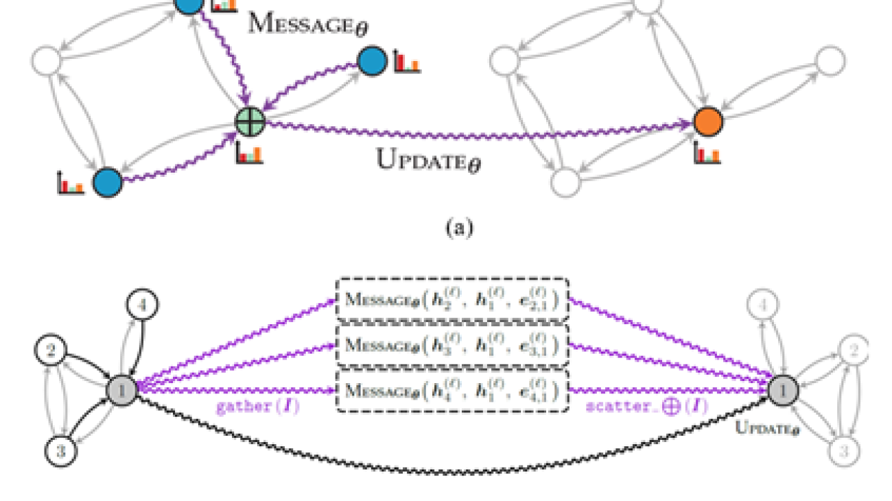
Message Passing Paradigm
Message passing refers to the process of nodes exchanging information with their respective neighbors by sending messages to one another. In PyG, the process of message passing can be generalized into three steps:
- Gather: Collect edge-level information of adjacent nodes and edges.
- Apply: Update the collected information with user-defined functions (UDFs).
- Scatter: Aggregate to node-level information, e.g., via a particular reduce function such as sum, mean, or max.
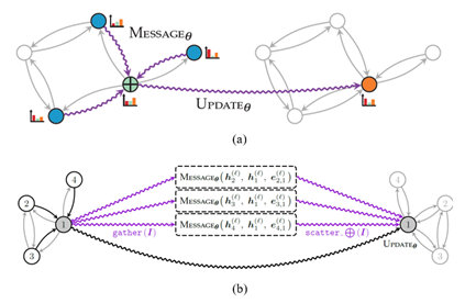
Figure 1: The message passing paradigm (Source: Matthias Fey)
Message passing performance is highly related to the storage format of the adjacency matrix of the graph, which records how pairs of nodes are connected. Two methods for the storage format are:
- Adjacency matrix in COO (Coordinate Format): The graph data is physically stored in a two-dimensional tensor shape of [2, num_edges], which maps each connection of source and destination nodes. The performance hotspot is scatter-reduce.
- Adjacency matrix in CSR (Compressed Sparse Row): Similar format to COO, but compressed on the row indices. This format allows for more efficient row access and faster sparse matrix-matrix multiplication (SpMM). The performance hotspot is sparse matrix related reduction ops.
Scatter-Reduce
The pattern of scatter-reduce is parallel in nature, which updates values of a self tensor using values from a src tensor at the entries specified by index. Ideally, parallelizing on the outer dimension would be most performant. However, direct parallelization leads to write conflicts, as different threads might try to update the same entry simultaneously.
Figure 2: Scatter-reduce and its optimization scheme (Source: Mingfei Ma)
To optimize this kernel, we use sorting followed by a reduction:
- Sorting: Sort the index tensor in ascending order with parallel radix sort, such that indices pointing to the same entry in the self tensor are managed in the same thread.
- Reduction: Paralleled on the outer dimension of self, and do vectorized reduction for each indexed src entry.
For its backward path during the training process (i.e., gather), sorting is not needed because its memory access pattern will not lead to any write conflicts.
SpMM-Reduce
Sparse matrix-matrix reduction is a fundamental operator in GNNs, where A is sparse adjacency matrix in CSR format and B is a dense feature matrix where the reduction type could be sum, mean or max.
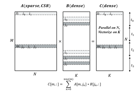
Figure 3: SpMM optimization scheme (Source: Mingfei Ma)
The biggest challenge when optimizing this kernel is how to balance thread payload when parallelizing along rows of the sparse matrix A. Each row in A corresponds to a node, and its number of connections may vary vastly from one to another; this results in thread payload imbalance. One technique to address such issues is to do payload scanning before thread partition. Aside from that, other techniques are also introduced to further exploit CPU performance such as vectorization and unrolling and blocking.
These optimizations are done via torch.sparse.mm using the reduce flags of amax, amin, mean, sum.
Performance Gains: Up to 4.1x Speedup
We collected benchmark performance for both inference and training in pytorch_geometric/benchmark and in the Open Graph Benchmark (OGB) to demonstrate the performance improvement from the above-mentioned methods on Intel® Xeon® Platinum 8380 Processor.
| Model – Dataset | Option | Speedup ratio |
| GCN-Reddit (inference) | 512-2-64-dense | 1.22x |
| 1024-3-128-dense | 1.25x | |
| 512-2-64-sparse | 1.31x | |
| 1024-3-128-sparse | 1.68x | |
| GraphSage-ogbn-products (inference) | 1024-3-128-dense | 1.15x |
| 512-2-64-sparse | 1.20x | |
| 1024-3-128-sparse | 1.33x | |
| full-batch-sparse | 4.07x | |
| GCN-PROTEINS (training) | 3-32 | 1.67x |
| GCN-REDDIT-BINARY (training) | 3-32 | 1.67x |
| GCN-Reddit (training) | 512-2-64-dense | 1.20x |
| 1024-3-128-dense | 1.12x |
Table 1: Performance Speedup on PyG Benchmark1
From the benchmark results, we can see that our optimizations in PyTorch and PyG achieved 1.1x-4.1x speed-up for inference and training.
torch.compile for PyG
The PyTorch2.0 flagship feature torch.compile is fully compatible with PyG 2.3 release, bringing additional speed-up in PyG model inference/training over imperative mode, thanks to TorchInductor C++/OpenMP backend for CPUs. In particular, a 3.0x – 5.4x performance speed-up is measured on basic GNN models with Intel Xeon Platinum 8380 Processor on model training2.
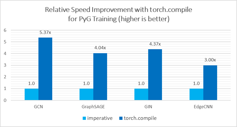
Figure 4: Performance Speedup with Torch Compile
Torch.compile can fuse the multiple stages of message passing into a single kernel, which provides significant speedup due to the saved memory bandwidth. Refer to this pytorch geometric tutorial for additional support.
Please note that torch.compile within PyG is in beta mode and under active development. Currently, some features do not yet work together seamlessly such as torch.compile(model, dynamic=True), but fixes are on the way from Intel.
Conclusion & Future Work
In this blog, we introduced the GNN performance optimizations included in PyTorch 2.0 on CPU. We are closely collaborating with the PyG community for future optimization work, which will focus on in-depth optimizations from torch.compile, sparse optimization, and distributed training.
Acknowledgement
The results presented in this blog is a joint effort of Intel PyTorch team and Kumo. Special thanks to Matthias Fey (Kumo), Pearu Peterson (Quansight) and Christian Puhrsch (Meta) who spent precious time and gave substantial assistance! Together, we made one more step forward on the path of improving the PyTorch CPU ecosystem.
References
- Accelerating PyG on Intel CPUs
- PyG 2.3.0: PyTorch 2.0 support, native sparse tensor support, explainability and accelerations
Footnotes
Product and Performance Information
1Platinum 8380: 1-node, 2x Intel Xeon Platinum 8380 processor with 256GB (16 slots/ 16GB/3200) total DDR4 memory, uCode 0xd000389, HT on, Turbo on, Ubuntu 20.04.5 LTS, 5.4.0-146-generic, INTEL SSDPE2KE016T8 1.5T; GCN + Reddit FP32 inference, GCN+Reddit FP32 training, GraphSAGE + ogbn-products FP32 inference, GCN-PROTAIN, GCN-REDDIT-BINARY FP32 training; Software: PyTorch 2.1.0.dev20230302+cpu, pytorch_geometric 2.3.0, torch-scatter 2.1.0, torch-sparse 0.6.16, test by Intel on 3/02/2023.
2Platinum 8380: 1-node, 2x Intel Xeon Platinum 8380 processor with 256GB (16 slots/ 16GB/3200) total DDR4 memory, uCode 0xd000389, HT on, Turbo on, Ubuntu 20.04.5 LTS, 5.4.0-146-generic, INTEL SSDPE2KE016T8 1.5T; GCN, GraphSAGE, GIN and EdgeCNN, FP32; Software: PyTorch 2.1.0.dev20230411+cpu, pytorch_geometric 2.4.0, torch-scatter 2.1.1+pt20cpu, torch-sparse 0.6.17+pt20cpu, test by Intel on 4/11/2023.
3Performance varies by use, configuration and other factors. Learn more at www.Intel.com/PerformanceIndex.
Do large language models really need all those layers?
Finding that 70% of attention heads and 20% of feed-forward networks can be excised with minimal effect on in-context learning suggests that large language models are undertrained.Read More

Research Focus: Week of July 3, 2023

Welcome to Research Focus, a series of blog posts that highlights notable publications, events, code/datasets, new hires and other milestones from across the research community at Microsoft.
NEW RESEARCH
The Best of Both Worlds: Unlocking the Potential of Hybrid Work for Software Engineers
The era of hybrid work has created new challenges and opportunities for developers. Their ability to choose where they work and the scheduling flexibility that comes with remote work can be offset by the loss of social interaction, reduced collaboration efficiency and difficulty separating work time from personal time. Companies must be equipped to maintain a successful and efficient hybrid workforce by accentuating the positive elements of hybrid work, while also addressing the challenges.
In a new study: The Best of Both Worlds: Unlocking the Potential of Hybrid Work for Software Engineers, researchers from Microsoft aim to identify which form of work – whether fully in office, fully at home, or blended – yields the highest productivity and job satisfaction among developers. They analyzed over 3,400 survey responses conducted across 28 companies in seven countries, in partnership with Vista Equity Partners, a leading global asset manager with experience investing in software, data, and technology-enabled organizations.
The study found that developers face many of the same challenges found in other types of hybrid workplaces. The researchers provide recommendations for addressing these challenges and unlocking more productivity while improving employee satisfaction.
Spotlight: Microsoft Research Podcast
AI Frontiers: The Physics of AI with Sébastien Bubeck
What is intelligence? How does it emerge and how do we measure it? Ashley Llorens and machine learning theorist Sébastian Bubeck discuss accelerating progress in large-scale AI and early experiments with GPT-4.
NEW INSIGHTS
Prompt Engineering: Improving our ability to communicate with LLMs
Pretrained natural language generation (NLG) models are powerful, but in the absence of contextual information, responses are necessarily generic. The prompt is the primary mechanism for access to NLG capabilities. It is an enormously effective and flexible tool, yet in order to be actively converted to the expected output, a prompt must meet expectations for how information is conveyed. If the prompt is not accurate and precise, the model is left guessing. Prompt engineering aims to bring more context and specificity to generative AI models, providing enough information in the model instructions that the user gets the exact result they want.
In a recent blog post: Prompt Engineering: Improving our Ability to Communicate with an LLM, researchers from Microsoft explain how they use retrieval augmented generation (RAG) to do knowledge grounding, use advanced prompt engineering to properly set context in the input to guide large language models (LLMs), implement a provenance check for responsible AI, and help users deploy scalable NLG service more safely, effectively, and efficiently.
NEW RESOURCE
Overwatch: Learning patterns in code edit sequences
Integrated development environments (IDEs) provide tool support to automate many source code editing tasks. IDEs typically use only the spatial context, i.e., the location where the developer is editing, to generate candidate edit recommendations. However, spatial context alone is often not sufficient to confidently predict the developer’s next edit, and thus IDEs generate many suggestions at a location. Therefore, IDEs generally do not actively offer suggestions. The developer must click on a specific icon or menu and then select from a large list of potential suggestions. As a consequence, developers often miss the opportunity to use the tool support because they are not aware it exists or forget to use it. To better understand common patterns in developer behavior and produce better edit recommendations, tool builders can use the temporal context, i.e., the edits that a developer was recently performing.
To enable edit recommendations based on temporal context, researchers from Microsoft created Overwatch, a novel technique for learning edit sequence patterns from traces of developers’ edits performed in an IDE. Their experiments show that Overwatch has 78% precision and that it not only completed edits when developers missed the opportunity to use the IDE tool support, but also predicted new edits that have no tool support in the IDE.
UPDATED RESOURCE
Qlib updates harness adaptive market dynamics modeling and reinforcement learning to address key challenges in financial markets
Qlib is an open-source framework built by Microsoft Research that empowers research into AI technologies applicable to the financial industry. Qlib initially supported diverse machine learning modeling paradigms, including supervised learning. Now, a series of recent updates have added support for market dynamics modeling and reinforcement learning, enabling researchers and engineers to tap into more sophisticated learning methods for advanced trading system construction.
These updates broaden Qlib’s capabilities and its value proposition for researchers and engineers, empowering them to explore ideas and implement effective quantitative trading strategies. The updates, available on GitHub, make Qlib the first platform to offer diverse learning paradigms aimed at helping researchers and engineers solve key financial market challenges.
A significant update is the introduction of adaptive concept drift technology for modeling the dynamic nature of financial markets. This feature can help researchers and engineers invent and implement algorithms that can adapt to changes in market trends and behavior over time, which is crucial for maintaining a competitive advantage in trading strategies.
Qlib’s support for reinforcement learning enables a new feature designed to model continuous investment decisions. This feature assists researchers and engineers in optimizing their trading strategies by learning from interactions with the environment to maximize some notion of cumulative reward.
Related research:
DDG-DA: Data Distribution Generation for Predictable Concept Drift Adaptation
Universal Trading for Order Execution with Oracle Policy Distillation
The post Research Focus: Week of July 3, 2023 appeared first on Microsoft Research.

Modular visual question answering via code generation
Visual question answering (VQA) is a machine learning task that requires a model to answer a question about an image or a set of images. Conventional VQA approaches need a large amount of labeled training data consisting of thousands of human-annotated question-answer pairs associated with images. In recent years, advances in large-scale pre-training have led to the development of VQA methods that perform well with fewer than fifty training examples (few-shot) and without any human-annotated VQA training data (zero-shot). However, there is still a significant performance gap between these methods and state-of-the-art fully supervised VQA methods, such as MaMMUT and VinVL. In particular, few-shot methods struggle with spatial reasoning, counting, and multi-hop reasoning. Furthermore, few-shot methods have generally been limited to answering questions about single images.
To improve accuracy on VQA examples that involve complex reasoning, in “Modular Visual Question Answering via Code Generation,” to appear at ACL 2023, we introduce CodeVQA, a framework that answers visual questions using program synthesis. Specifically, when given a question about an image or set of images, CodeVQA generates a Python program (code) with simple visual functions that allow it to process images, and executes this program to determine the answer. We demonstrate that in the few-shot setting, CodeVQA outperforms prior work by roughly 3% on the COVR dataset and 2% on the GQA dataset.
CodeVQA
The CodeVQA approach uses a code-writing large language model (LLM), such as PALM, to generate Python programs (code). We guide the LLM to correctly use visual functions by crafting a prompt consisting of a description of these functions and fewer than fifteen “in-context” examples of visual questions paired with the associated Python code for them. To select these examples, we compute embeddings for the input question and of all of the questions for which we have annotated programs (a randomly chosen set of fifty). Then, we select questions that have the highest similarity to the input and use them as in-context examples. Given the prompt and question that we want to answer, the LLM generates a Python program representing that question.
We instantiate the CodeVQA framework using three visual functions: (1) query, (2) get_pos, and (3) find_matching_image.
Query, which answers a question about a single image, is implemented using the few-shot Plug-and-Play VQA (PnP-VQA) method. PnP-VQA generates captions using BLIP — an image-captioning transformer pre-trained on millions of image-caption pairs — and feeds these into a LLM that outputs the answers to the question.Get_pos, which is an object localizer that takes a description of an object as input and returns its position in the image, is implemented using GradCAM. Specifically, the description and the image are passed through the BLIP joint text-image encoder, which predicts an image-text matching score. GradCAM takes the gradient of this score with respect to the image features to find the region most relevant to the text.Find_matching_image, which is used in multi-image questions to find the image that best matches a given input phrase, is implemented by using BLIP text and image encoders to compute a text embedding for the phrase and an image embedding for each image. Then the dot products of the text embedding with each image embedding represent the relevance of each image to the phrase, and we pick the image that maximizes this relevance.
The three functions can be implemented using models that require very little annotation (e.g., text and image-text pairs collected from the web and a small number of VQA examples). Furthermore, the CodeVQA framework can be easily generalized beyond these functions to others that a user might implement (e.g., object detection, image segmentation, or knowledge base retrieval).
 |
Illustration of the CodeVQA method. First, a large language model generates a Python program (code), which invokes visual functions that represent the question. In this example, a simple VQA method (query) is used to answer one part of the question, and an object localizer (get_pos) is used to find the positions of the objects mentioned. Then the program produces an answer to the original question by combining the outputs of these functions. |
Results
The CodeVQA framework correctly generates and executes Python programs not only for single-image questions, but also for multi-image questions. For example, if given two images, each showing two pandas, a question one might ask is, “Is it true that there are four pandas?” In this case, the LLM converts the counting question about the pair of images into a program in which an object count is obtained for each image (using the query function). Then the counts for both images are added to compute a total count, which is then compared to the number in the original question to yield a yes or no answer.
 |
We evaluate CodeVQA on three visual reasoning datasets: GQA (single-image), COVR (multi-image), and NLVR2 (multi-image). For GQA, we provide 12 in-context examples to each method, and for COVR and NLVR2, we provide six in-context examples to each method. The table below shows that CodeVQA improves consistently over the baseline few-shot VQA method on all three datasets.
| Method | GQA | COVR | NLVR2 | ||||||||
| Few-shot PnP-VQA | 46.56 | 49.06 | 63.37 | ||||||||
| CodeVQA | 49.03 | 54.11 | 64.04 |
| Results on the GQA, COVR, and NLVR2 datasets, showing that CodeVQA consistently improves over few-shot PnP-VQA. The metric is exact-match accuracy, i.e., the percentage of examples in which the predicted answer exactly matches the ground-truth answer. |
We find that in GQA, CodeVQA’s accuracy is roughly 30% higher than the baseline on spatial reasoning questions, 4% higher on “and” questions, and 3% higher on “or” questions. The third category includes multi-hop questions such as “Are there salt shakers or skateboards in the picture?”, for which the generated program is shown below.
img = open_image("Image13.jpg")
salt_shakers_exist = query(img, "Are there any salt shakers?")
skateboards_exist = query(img, "Are there any skateboards?")
if salt_shakers_exist == "yes" or skateboards_exist == "yes":
    answer = "yes"
else:
    answer = "no"
In COVR, we find that CodeVQA’s gain over the baseline is higher when the number of input images is larger, as shown in the table below. This trend indicates that breaking the problem down into single-image questions is beneficial.
| Number of images | |||||||||||
| Method | 1 | 2 | 3 | 4 | 5 | ||||||
| Few-shot PnP-VQA | 91.7 | 51.5 | 48.3 | 47.0 | 46.9 | ||||||
| CodeVQA | 75.0 | 53.3 | 48.7 | 53.2 | 53.4 | ||||||
Conclusion
We present CodeVQA, a framework for few-shot visual question answering that relies on code generation to perform multi-step visual reasoning. Exciting directions for future work include expanding the set of modules used and creating a similar framework for visual tasks beyond VQA. We note that care should be taken when considering whether to deploy a system such as CodeVQA, since vision-language models like the ones used in our visual functions have been shown to exhibit social biases. At the same time, compared to monolithic models, CodeVQA offers additional interpretability (through the Python program) and controllability (by modifying the prompts or visual functions), which are useful in production systems.
Acknowledgements
This research was a collaboration between UC Berkeley’s Artificial Intelligence Research lab (BAIR) and Google Research, and was conducted by Sanjay Subramanian, Medhini Narasimhan, Kushal Khangaonkar, Kevin Yang, Arsha Nagrani, Cordelia Schmid, Andy Zeng, Trevor Darrell, and Dan Klein.