The system has expanded from generating peak computation-load forecasts one year in advance to a series of forecasts that include per-minute forecasts several months into the future.Read More

MAXimum AI Performance: Latest Adobe Updates Accelerated by NVIDIA GPUs Improve Workflows for Millions of Creatives
Generative AI is helping creatives across many industries bring ideas to life at unprecedented speed.
This technology will be on display at Adobe MAX, running through Thursday, Oct. 12, in person and virtually.
Adobe is putting the power of generative AI into the hands of creators with the release of Adobe Firefly. Using NVIDIA GPUs, Adobe is bringing new opportunities for artists and more looking to accelerate generative AI — unleashing generative AI enhancements for millions of users. Firefly is now available as a standalone app and integrated with other Adobe apps.
Recent updates to Adobe’s most popular apps — including for Adobe Premiere Pro, Lightroom, After Effects and Substance 3D Stager, Modeler and Sampler — bring new AI features to creators. And GeForce RTX and NVIDIA RTX GPUs help accelerate these apps and AI effects, providing massive time savings.
Video editors can use AI to improve dialogue quality with the Enhance Speech (beta) function and work faster with GPU accelerated decoding of ARRIRAW camera original digital film clips up to 60% faster on RTX GPUs compared to on an Apple MacBook Pro 16 M2 Max in Premiere Pro. Plus, take advantage of improved rotoscoping quality with the Next-Gen Roto Brush (version 3.0) feature now available in After Effects.
Photographers and 2D artists now have new Lens Blur effects in Lightroom, complementing ongoing optimizations that improve performance in its Select Object, Select People and Select Sky features.
These advanced features are further enhanced by NVIDIA Studio Drivers, free for RTX GPU owners, which add performance and reliability. The October Studio Driver is available for download now.
Finally, 3D artist SouthernShotty returns to In the NVIDIA Studio to share his 3D montage of a mix of beautifully hand-crafted worlds — built with Adobe apps and Blender and featuring AI-powered workflows accelerated by his GeForce RTX 4090 Laptop GPU.
MAXimizing Creativity
Adobe Creative Cloud and Substance 3D apps run fastest on NVIDIA RTX GPUs — and recent updates show continued time-saving performance gains.
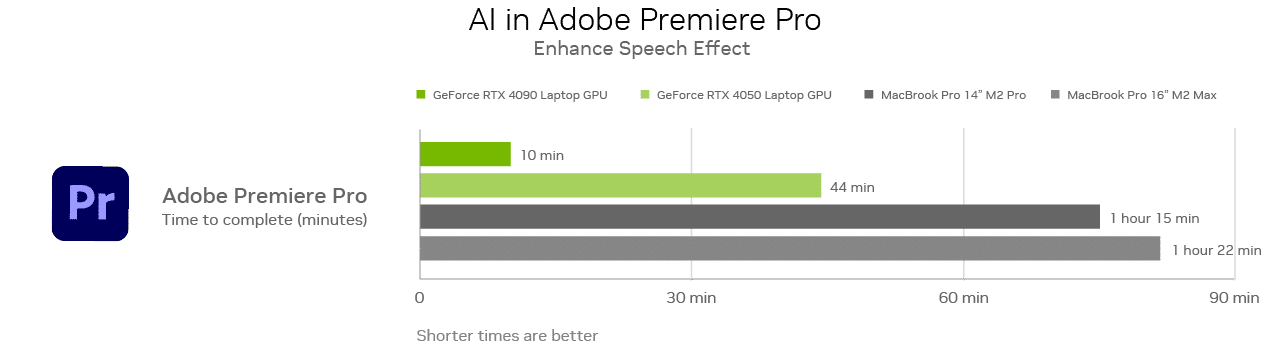
Premiere Pro’s Enhance Speech (beta) feature, currently in beta, uses AI to remove noise and improve the quality of dialogue clips so that they sound professionally recorded. Tasks are completed 8x faster with a GeForce RTX 4090 Laptop GPU compared to MacBook Pro 16 with M2 Max.

Premiere Pro professionals use ARRIRAW footage — the only format that fully retains a camera’s natural color response and great exposure latitude. ARRIRAW video exports can be done 1.6x faster on GeForce RTX 4090 Laptop GPUs than on the MacBook Pro 16 with M2 Max.
Additionally, After Effects users can access the Next-Gen Roto Brush feature in beta, powered by a brand-new AI model. It’s ideal for isolating subjects such as overlapping limbs, hair and other transparencies more easily, saving time.
RTX GPUs shine in 3D workloads. Substance 3D Stager’s new AI-powered, GPU-accelerated denoiser allows almost instantaneous photorealistic rendering.
Substance 3D Modeler’s recent Hardware Ray Tracing in Capture Mode capability uses NVIDIA technology to export high-quality screenshots 2.4x faster than before.
Meanwhile, Substance 3D Sampler’s AI UpScale feature increases detail for low-quality textures and its Image to Material feature makes it easier to create high-quality materials from a single photograph.
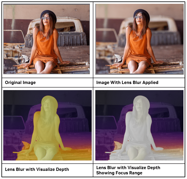
Photographers have long used the popular Super Resolution feature in Adobe Camera Raw, which is supported by Photoshop, and gives 3x faster performance on a GeForce RTX 4090 Laptop GPU compared to a MacBook Pro 16 M2 Max. Now, Lightroom users have AI-driven capabilities with the Lens Blur feature for applying realistic lens blur effects, Point Color for precise color adjustments to speed up color correction, and High Dynamic Range Output for edits and renders in an HDR color space.
Adobe Firefly Glows #76B900
Adobe Firefly provides users with generative AI features, utilizing NVIDIA GPUs in the cloud.
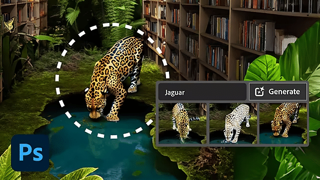
Firefly features such as Generative Fill — to add, remove and expand content in Photoshop, and Generative Expand to expand scenes with generative content — help complete tasks instantly in Adobe Photoshop.
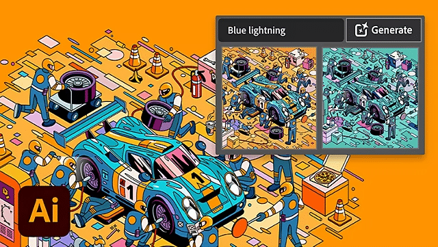
Adobe Illustrator offers the Generative Recolor feature, which enables graphic designers to explore a wide variety of colors, palettes and themes in their work without having to do tedious manual recoloring. Discovering the perfect combination of colors now takes just a few seconds.
Adobe Express offers the Text to Image feature to create incredible imagery from standard prompts, and the Text Effects feature helps stylize standard text for use in creating flyers, resumes, social media reels and more.
These powerful AI capabilities were developed with the creative community in mind — guided by AI ethics principles of content and data transparency — to ensure ethically and morally responsible output.
NVIDIA technology will continue to support new Adobe Firefly-powered features from the cloud as they become available to photographers, illustrators, designers, video editors, 3D artists and more.
MAXed Out AI Fun
Independent filmmaker and artist SouthernShotty knows the challenges of producing content alone and how daunting the process can be.

“I’m a big fan of the NVIDIA Studio Driver support, because it adds stability and reliability.” – SouthernShotty
As such, SouthernShotty is always looking for tools and techniques to ease the creative process. To accelerate his workflow, he combined new Adobe AI capabilities accelerated by his GeForce RTX 4090 GPU to achieve incredible efficiency.
The artist kept his 3D models fairly simple, focusing on textures to ensure that the world would match his vision. He deployed one of his favorite features, the AI-powered Image to Material in Adobe Substance 3D Sampler, to convert images to physically based rendering textures.
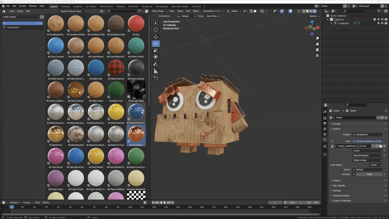
“It’s so fast that I can pretty much preview my entire scene in real time and see the final result before I ever hit the render button.” – SouthernShotty
RTX-accelerated light and ambient occlusion baking allowed SouthernShotty to realize the desired visual effect in seconds.
His RTX GPU continued to play an essential role as he used Blender Cycles’ RTX-accelerated OptiX ray tracing in the viewport for interactive, photorealistic rendering.
As the 3D montage progresses, the main character appears and reappears in several new environments. Each new location is featured for only a second or two, but SouthernShotty still needed to create a fully fleshed out environment for each.
Normally this would take a substantial amount of time, but an AI assist from Adobe Firefly helped speed the process.
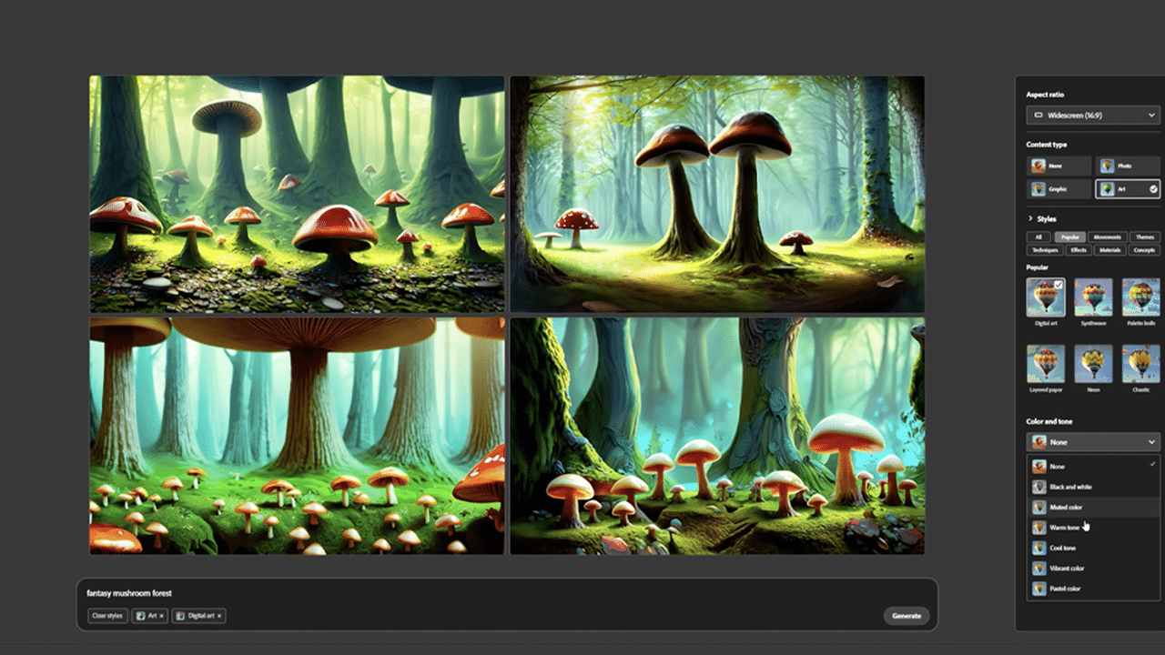
SouthernShotty opened the app, entered “fantasy mushroom forest” as the text prompt and then made minor adjustments by tinkering with the digital art, golden hour, for lighting, and wide-angle settings for composition. When satisfied with the result, he downloaded the image for further editing in Photoshop.

SouthernShotty then used the AI-powered Generative Fill feature to remove unwanted background elements. He used the Neural Filters optimization to color match a castle element added in the background, then used Generative Fill again to effortlessly blend the castle in with the trees.
Finally, SouthernShotty used the Neural Filters optimization in the new Lens Blur feature to add depth to the scene — first exporting depth as a separate layer and then editing in Blender to complete the scene.
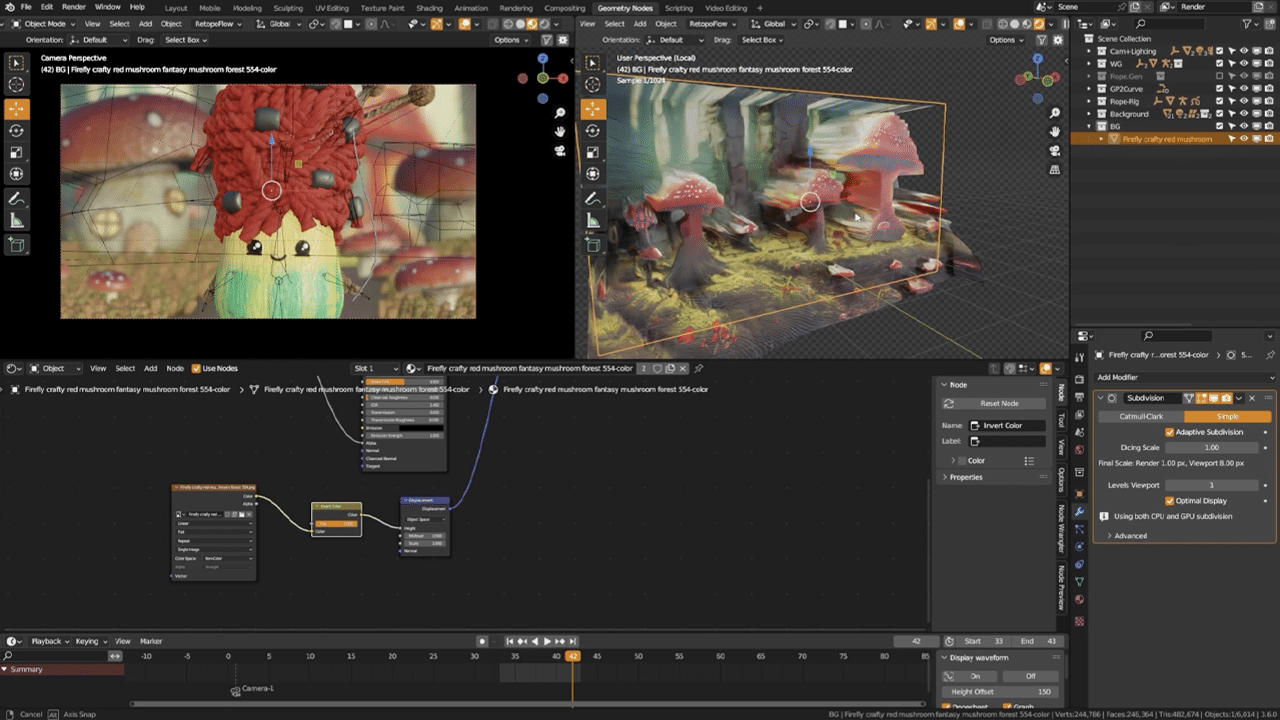
“My entire process was sprinkled with GPU-acceleration and AI-enabled features,” said SouthernShotty. “In Blender, the GeForce RTX 4090 GPU accelerated everything — but especially the live render view in my viewport, which was crucial to visualizing my scenes.”
Check out SouthernShotty’s YouTube channel for Blender tutorials on characters, animation, rigging and more.
Follow NVIDIA Studio on Instagram, Twitter and Facebook. Access tutorials on the Studio YouTube channel and get updates directly in your inbox by subscribing to the Studio newsletter.

New ways we’re helping reduce transportation and energy emissions
 These new product features and expansions help people, city planners and policy makers take action toward building a sustainable future.Read More

Demand more from social with AI-powered ads
 Learn how Demand Gen campaigns can help you drive better results across YouTube and Google. See new case studies, videos, tips, and more.Read More
Real-time Audio-visual Speech Recognition
Audio-Visual Speech Recognition (AV-ASR, or AVSR) is the task of transcribing text from audio and visual streams, which has recently attracted a lot of research attention due to its robustness to noise. The vast majority of work to date has focused on developing AV-ASR models for non-streaming recognition; studies on streaming AV-ASR are very limited.
We have developed a compact real-time speech recognition system based on TorchAudio, a library for audio and signal processing with PyTorch. It can run locally on a laptop with high accuracy without accessing the cloud. Today, we are releasing the real-time AV-ASR recipe under a permissive open license (BSD-2-Clause license), enabling a broad set of applications and fostering further research on audio-visual models for speech recognition.
This work is part of our approach to AV-ASR research. A promising aspect of this approach is its ability to automatically annotate large-scale audio-visual datasets, which enables the training of more accurate and robust speech recognition systems. Furthermore, this technology has the potential to run on smart devices since it achieves the latency and memory efficiency that such devices require for inference.
In the future, speech recognition systems are expected to power applications in numerous domains. One of the primary applications of AV-ASR is to enhance the performance of ASR in noisy environments. Since visual streams are not affected by acoustic noise, integrating them into an audio-visual speech recognition model can compensate for the performance drop of ASR models. Our AV-ASR system has the potential to serve multiple purposes beyond speech recognition, such as text summarization, translation and even text-to-speech conversion. Moreover, the exclusive use of VSR can be useful in certain scenarios, e.g. where speaking is not allowed, in meetings, and where privacy in public conversations is desired.
AV-ASR
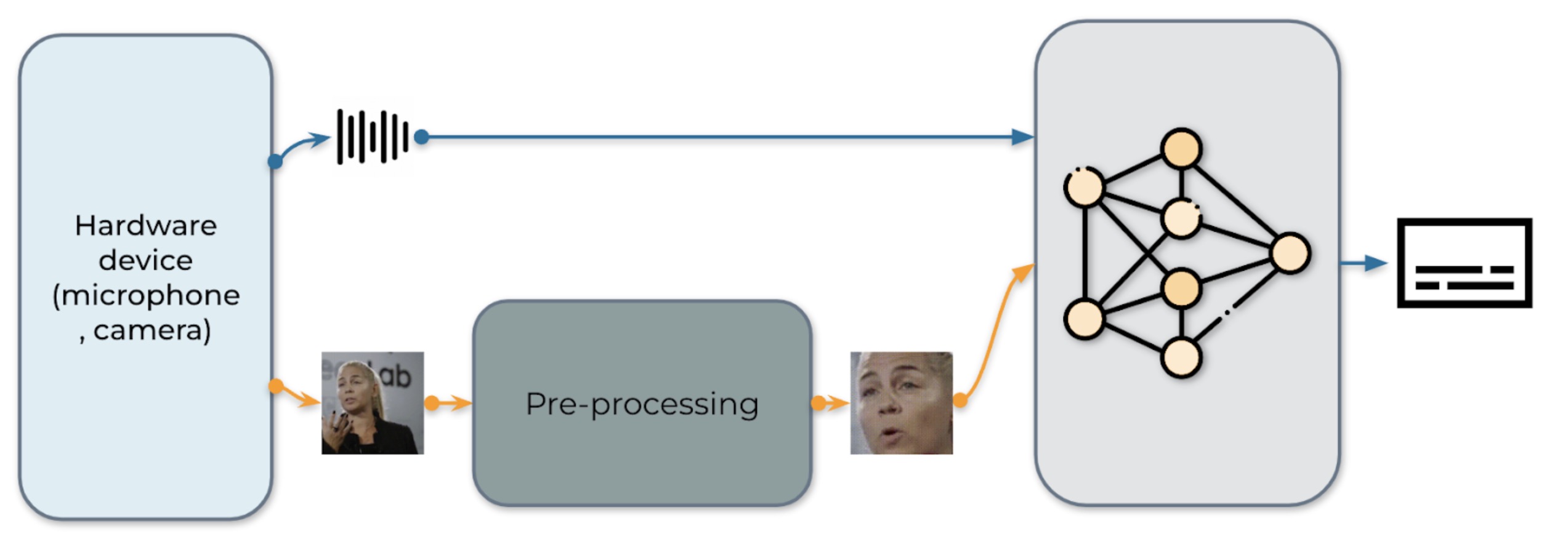
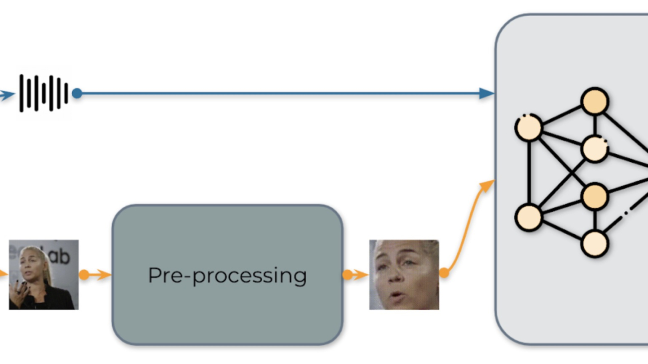
Fig. 1: The pipeline for audio-visual speech recognition system
Our real-time AV-ASR system is presented in Fig. 1. It consists of three components, a data collection module, a pre-processing module and an end-to-end model. The data collection module comprises hardware devices, such as a microphone and camera. Its role is to collect information from the real world. Once the information is collected, the pre-processing module location and crop out face. Next, we feed the raw audio stream and the pre-processed video stream into our end-to-end model for inference.
Data collection
We use torchaudio.io.StreamReader to capture audio/video from streaming device input, e.g. microphone and camera on laptop. Once the raw video and audio streams are collected, the pre-processing module locates and crops faces. It should be noted that data is immediately deleted during the streaming process.
Pre-processing
Before feeding the raw stream into our model, each video sequence has to undergo a specific pre-processing procedure. This involves three critical steps. The first step is to perform face detection. Following that, each individual frame is aligned to a referenced frame, commonly known as the mean face, in order to normalize rotation and size differences across frames. The final step in the pre-processing module is to crop the face region from the aligned face image. We would like to clearly note that our model is fed with raw audio waveforms and pixels of the face, without any further preprocessing like face parsing or landmark detection. An example of the pre-processing procedure is illustrated in Table 1.
 |
|
 |
 |
| 0. Original | 1. Detection | 2. Alignment | 3. Crop |
Table 1: Preprocessing pipeline.
Model
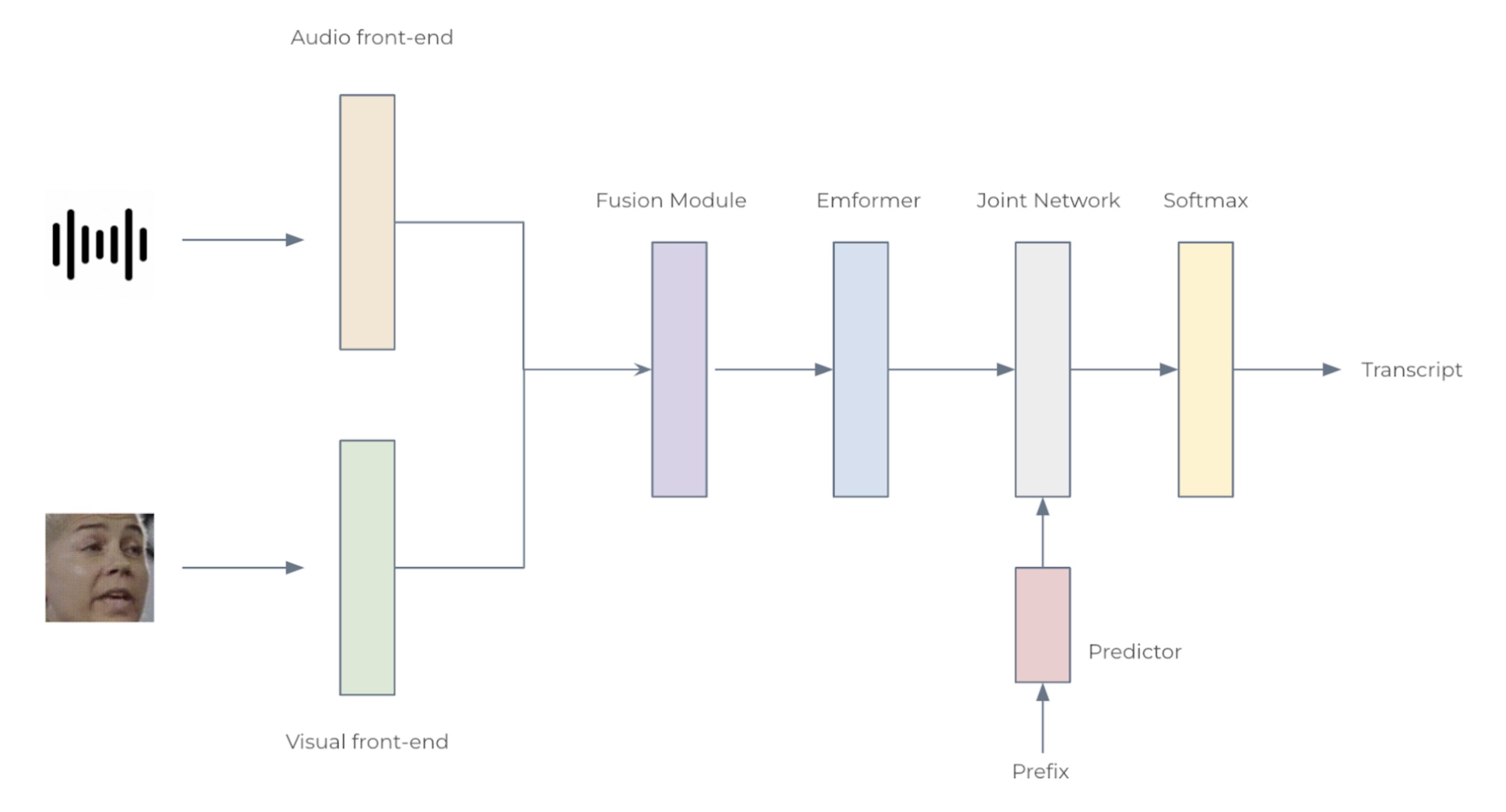
Fig. 2: The architecture for the audio-visual speech recognition system
We consider two configurations: Small with 12 Emformer blocks and Large with 28, with 34.9M and 383.3M parameters, respectively. Each AV-ASR model composes front-end encoders, a fusion module, an Emformer encoder, and a transducer model. To be specific, we use convolutional frontends to extract features from raw audio waveforms and facial images. The features are concatenated to form 1024-d features, which are then passed through a two-layer multi-layer perceptron and an Emformer transducer model. The entire network is trained using RNN-T loss. The architecture of the proposed AV-ASR model is illustrated in Fig. 2.
Analysis
Datasets. We follow Auto-AVSR: Audio-Visual Speech Recognition with Automatic Labels to use publicly available audio-visual datasets including LRS3, VoxCeleb2 and AVSpeech for training. We do not use mouth ROIs or facial landmarks or attributes during both training and testing stages.
Comparisons with the state-of-the-art. Non-streaming evaluation results on LRS3 are presented in Table 2. Our audio-visual model with an algorithmic latency of 800 ms (160ms+1280msx0.5) yields a WER of 1.3%, which is on par with those achieved by state-of-the-art offline models such as AV-HuBERT, RAVEn, and Auto-AVSR.
| Method | Total Hours | WER (%) |
| ViT3D-CM | 90, 000 | 1.6 |
| AV-HuBERT | 1, 759 | 1.4 |
| RAVEn | 1, 759 | 1.4 |
| AutoAVSR | 3, 448 | 0.9 |
| Ours | 3, 068 | 1.3 |
Table 2: Non-streaming evaluation results for audio-visual models on the LRS3 dataset.
Noisy experiments. During training, 16 different noise types are randomly injected to audio waveforms, including 13 types from Demand database, ‘DLIVING’,’DKITCHEN’, ‘OMEETING’, ‘OOFFICE’, ‘PCAFETER’, ‘PRESTO’, ‘PSTATION’, ‘STRAFFIC’, ‘SPSQUARE’, ‘SCAFE’, ‘TMETRO’, ‘TBUS’ and ‘TCAR’, two more types of noise from speech commands database, white and pink and one more type of noise from NOISEX-92 database, babble noise. SNR levels in the range of [clean, 7.5dB, 2.5dB, -2.5dB, -7.5dB] are selected from with a uniform distribution. Results of ASR and AV-ASR models, when tested with babble noise, are shown in Table 3. With increasing noise level, the performance advantage of our audio-visual model over our audio-only model grows, indicating that incorporating visual data improves noise robustness.
| Type | ∞ | 10dB | 5dB | 0dB | -5dB | -10dB |
| A | 1.6 | 1.8 | 3.2 | 10.9 | 27.9 | 55.5 |
| A+V | 1.6 | 1.7 | 2.1 | 6.2 | 11.7 | 27.6 |
Table 3: Streaming evaluation WER (%) results at various signal-to-noise ratios for our audio-only (A) and audio-visual (A+V) models on the LRS3 dataset under 0.80-second latency constraints.
Real-time factor. The real-time factor (RTF) is an important measure of a system’s ability to process real-time tasks efficiently. An RTF value of less than 1 indicates that the system meets real-time requirements. We measure RTF using a laptop with an Intel® Core™ i7-12700 CPU running at 2.70 GHz and an NVIDIA 3070 GeForce RTX 3070 Ti GPU. To the best of our knowledge, this is the first AV-ASR model that reports RTFs on the LRS3 benchmark. The Small model achieves a WER of 2.6% and an RTF of 0.87 on CPU (Table 4), demonstrating its potential for real-time on-device inference applications.
| Model | Device | Streaming WER [%] | RTF |
| Large | GPU | 1.6 | 0.35 |
| Small | GPU | 2.6 | 0.33 |
| CPU | 0.87 |
Table 4: Impact of AV-ASR model size and device on WER and RTF. Note that the RTF calculation includes the pre-processing step wherein the Ultra-Lightweight Face Detection Slim 320 model is used to generate face bounding boxes.
Learn more about the system from the published works below:
- Shi, Yangyang, Yongqiang Wang, Chunyang Wu, Ching-Feng Yeh, Julian Chan, Frank Zhang, Duc Le, and Mike Seltzer. “Emformer: Efficient memory transformer based acoustic model for low latency streaming speech recognition.” In ICASSP 2021-2021 IEEE International Conference on Acoustics, Speech and Signal Processing (ICASSP), pp. 6783-6787. IEEE, 2021.
- Ma, Pingchuan, Alexandros Haliassos, Adriana Fernandez-Lopez, Honglie Chen, Stavros Petridis, and Maja Pantic. “Auto-AVSR: Audio-Visual Speech Recognition with Automatic Labels.” In ICASSP 2023-2023 IEEE International Conference on Acoustics, Speech and Signal Processing (ICASSP), pp. 1-5. IEEE, 2023.
Mistral 7B foundation models from Mistral AI are now available in Amazon SageMaker JumpStart
Today, we are excited to announce that the Mistral 7B foundation models, developed by Mistral AI, are available for customers through Amazon SageMaker JumpStart to deploy with one click for running inference. With 7 billion parameters, Mistral 7B can be easily customized and quickly deployed. You can try out this model with SageMaker JumpStart, a machine learning (ML) hub that provides access to algorithms and models so you can quickly get started with ML. In this post, we walk through how to discover and deploy the Mistral 7B model.
What is Mistral 7B
Mistral 7B is a foundation model developed by Mistral AI, supporting English text and code generation abilities. It supports a variety of use cases, such as text summarization, classification, text completion, and code completion. To demonstrate the easy customizability of the model, Mistral AI has also released a Mistral 7B Instruct model for chat use cases, fine-tuned using a variety of publicly available conversation datasets.
Mistral 7B is a transformer model and uses grouped-query attention and sliding-window attention to achieve faster inference (low latency) and handle longer sequences. Group query attention is an architecture that combines multi-query and multi-head attention to achieve output quality close to multi-head attention and comparable speed to multi-query attention. Sliding-window attention uses the stacked layers of a transformer to attend in the past beyond the window size to increase context length. Mistral 7B has an 8,000-token context length, demonstrates low latency and high throughput, and has strong performance when compared to larger model alternatives, providing low memory requirements at a 7B model size. The model is made available under the permissive Apache 2.0 license, for use without restrictions.
What is SageMaker JumpStart
With SageMaker JumpStart, ML practitioners can choose from a growing list of best-performing foundation models. ML practitioners can deploy foundation models to dedicated Amazon SageMaker instances within a network isolated environment, and customize models using SageMaker for model training and deployment.
You can now discover and deploy Mistral 7B with a few clicks in Amazon SageMaker Studio or programmatically through the SageMaker Python SDK, enabling you to derive model performance and MLOps controls with SageMaker features such as Amazon SageMaker Pipelines, Amazon SageMaker Debugger, or container logs. The model is deployed in an AWS secure environment and under your VPC controls, helping ensure data security.
Discover models
You can access Mistral 7B foundation models through SageMaker JumpStart in the SageMaker Studio UI and the SageMaker Python SDK. In this section, we go over how to discover the models in SageMaker Studio.
SageMaker Studio is an integrated development environment (IDE) that provides a single web-based visual interface where you can access purpose-built tools to perform all ML development steps, from preparing data to building, training, and deploying your ML models. For more details on how to get started and set up SageMaker Studio, refer to Amazon SageMaker Studio.
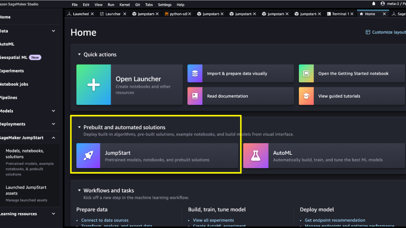
In SageMaker Studio, you can access SageMaker JumpStart, which contains pre-trained models, notebooks, and prebuilt solutions, under Prebuilt and automated solutions.

From the SageMaker JumpStart landing page, you can browse for solutions, models, notebooks, and other resources. You can find Mistral 7B in the Foundation Models: Text Generation carousel.

You can also find other model variants by choosing Explore all Text Models or searching for “Mistral.”

You can choose the model card to view details about the model such as license, data used to train, and how to use. You will also find two buttons, Deploy and Open notebook, which will help you use the model (the following screenshot shows the Deploy option).

Deploy models
Deployment starts when you choose Deploy. Alternatively, you can deploy through the example notebook that shows up when you choose Open notebook. The example notebook provides end-to-end guidance on how to deploy the model for inference and clean up resources.
To deploy using notebook, we start by selecting the Mistral 7B model, specified by the model_id. You can deploy any of the selected models on SageMaker with the following code:
This deploys the model on SageMaker with default configurations, including default instance type (ml.g5.2xlarge) and default VPC configurations. You can change these configurations by specifying non-default values in JumpStartModel. After it’s deployed, you can run inference against the deployed endpoint through the SageMaker predictor:
Optimizing the deployment configuration
Mistral models use Text Generation Inference (TGI version 1.1) model serving. When deploying models with the TGI deep learning container (DLC), you can configure a variety of launcher arguments via environment variables when deploying your endpoint. To support the 8,000-token context length of Mistral 7B models, SageMaker JumpStart has configured some of these parameters by default: we set MAX_INPUT_LENGTH and MAX_TOTAL_TOKENS to 8191 and 8192, respectively. You can view the full list by inspecting your model object:
By default, SageMaker JumpStart doesn’t clamp concurrent users via the environment variable MAX_CONCURRENT_REQUESTS smaller than the TGI default value of 128. The reason is because some users may have typical workloads with small payload context lengths and want high concurrency. Note that the SageMaker TGI DLC supports multiple concurrent users through rolling batch. When deploying your endpoint for your application, you might consider whether you should clamp MAX_TOTAL_TOKENS or MAX_CONCURRENT_REQUESTS prior to deployment to provide the best performance for your workload:
Here, we show how model performance might differ for your typical endpoint workload. In the following tables, you can observe that small-sized queries (128 input words and 128 output tokens) are quite performant under a large number of concurrent users, reaching token throughput on the order of 1,000 tokens per second. However, as the number of input words increases to 512 input words, the endpoint saturates its batching capacity—the number of concurrent requests allowed to be processed simultaneously—resulting in a throughput plateau and significant latency degradations starting around 16 concurrent users. Finally, when querying the endpoint with large input contexts (for example, 6,400 words) simultaneously by multiple concurrent users, this throughput plateau occurs relatively quickly, to the point where your SageMaker account will start encountering 60-second response timeout limits for your overloaded requests.
| . | throughput (tokens/s) | ||||||||||
| concurrent users | 1 | 2 | 4 | 8 | 16 | 32 | 64 | 128 | |||
| model | instance type | input words | output tokens | . | |||||||
| mistral-7b-instruct | ml.g5.2xlarge | 128 | 128 | 30 | 54 | 89 | 166 | 287 | 499 | 793 | 1030 |
| 512 | 128 | 29 | 50 | 80 | 140 | 210 | 315 | 383 | 458 | ||
| 6400 | 128 | 17 | 25 | 30 | 35 | — | — | — | — | ||
| . | p50 latency (ms/token) | ||||||||||
| concurrent users | 1 | 2 | 4 | 8 | 16 | 32 | 64 | 128 | |||
| model | instance type | input words | output tokens | . | |||||||
| mistral-7b-instruct | ml.g5.2xlarge | 128 | 128 | 32 | 33 | 34 | 36 | 41 | 46 | 59 | 88 |
| 512 | 128 | 34 | 36 | 39 | 43 | 54 | 71 | 112 | 213 | ||
| 6400 | 128 | 57 | 71 | 98 | 154 | — | — | — | — | ||
Inference and example prompts
Mistral 7B
You can interact with a base Mistral 7B model like any standard text generation model, where the model processes an input sequence and outputs predicted next words in the sequence. The following is a simple example with multi-shot learning, where the model is provided with several examples and the final example response is generated with contextual knowledge of these previous examples:
Mistral 7B instruct
The instruction-tuned version of Mistral accepts formatted instructions where conversation roles must start with a user prompt and alternate between user and assistant. A simple user prompt may look like the following:
A multi-turn prompt would look like the following:
This pattern repeats for however many turns are in the conversation.
In the following sections, we explore some examples using the Mistral 7B Instruct model.
Knowledge retrieval
The following is an example of knowledge retrieval:
Large context question answering
To demonstrate how to use this model to support large input context lengths, the following example embeds a passage, titled “Rats” by Robert Sullivan (reference), from the MCAS Grade 10 English Language Arts Reading Comprehension test into the input prompt instruction and asks the model a directed question about the text:
Mathematics and reasoning
The Mistral models also report strengths in mathematics accuracy. Mistral can provide comprehension such as the following math logic:
Coding
The following is an example of a coding prompt:
Clean up
After you’re done running the notebook, make sure to delete all the resources that you created in the process so your billing is stopped. Use the following code:
Conclusion
In this post, we showed you how to get started with Mistral 7B in SageMaker Studio and deploy the model for inference. Because foundation models are pre-trained, they can help lower training and infrastructure costs and enable customization for your use case. Visit Amazon SageMaker JumpStart now to get started.
Resources
- SageMaker JumpStart documentation
- SageMaker JumpStart foundation models documentation
- SageMaker JumpStart product detail page
- SageMaker JumpStart model catalog
About the Authors
 Dr. Kyle Ulrich is an Applied Scientist with the Amazon SageMaker JumpStart team. His research interests include scalable machine learning algorithms, computer vision, time series, Bayesian non-parametrics, and Gaussian processes. His PhD is from Duke University and he has published papers in NeurIPS, Cell, and Neuron.
 Dr. Ashish Khetan is a Senior Applied Scientist with Amazon SageMaker JumpStart and helps develop machine learning algorithms. He got his PhD from University of Illinois Urbana-Champaign. He is an active researcher in machine learning and statistical inference, and has published many papers in NeurIPS, ICML, ICLR, JMLR, ACL, and EMNLP conferences.
 Vivek Singh is a product manager with Amazon SageMaker JumpStart. He focuses on enabling customers to onboard SageMaker JumpStart to simplify and accelerate their ML journey to build generative AI applications.
 Roy Allela is a Senior AI/ML Specialist Solutions Architect at AWS based in Munich, Germany. Roy helps AWS customers—from small startups to large enterprises—train and deploy large language models efficiently on AWS. Roy is passionate about computational optimization problems and improving the performance of AI workloads.

SANPO: A Scene understanding, Accessibility, Navigation, Pathfinding, & Obstacle avoidance dataset

As most people navigate their everyday world, they process visual input from the environment using an eye-level perspective. Unlike robots and self-driving cars, people don’t have any “out-of-body” sensors to help guide them. Instead, a person’s sensory input is completely “egocentric”, or “from the self.” This also applies to new technologies that understand the world around us from a human-like perspective, e.g., robots navigating through unknown buildings, AR glasses that highlight objects, or assistive technology to help people run independently.
In computer vision, scene understanding is the subfield that studies how visible objects relate to the scene’s 3D structure and layout by focusing on the spatial, functional, and semantic relationships between objects and their environment. For example, autonomous drivers must understand the 3D structure of the road, sidewalks, and surrounding buildings while identifying and recognizing street signs and stop lights, a task made easier with 3D data from a special laser scanner mounted on the top of the car rather than 2D images from the driver’s perspective. Robots navigating a park must understand where the path is and what obstacles might interfere, which is simplified with a map of their surroundings and GPS positioning data. Finally, AR glasses that help users find their way need to understand where the user is and what they are looking at.
The computer vision community typically studies scene understanding tasks in contexts like self-driving, where many other sensors (GPS, wheel positioning, maps, etc.) beyond egocentric imagery are available. Yet most datasets in this space do not focus exclusively on egocentric data, so they are less applicable to human-centered navigation tasks. While there are plenty of self-driving focused scene understanding datasets, they have limited generalization to egocentric human scene understanding. A comprehensive human egocentric dataset would help build systems for related applications and serve as a challenging benchmark for the scene understanding community.
To that end, we present the Scene understanding, Accessibility, Navigation, Pathfinding, Obstacle avoidance dataset, or SANPO (also the Japanese word for ”brisk stroll”), a multi-attribute video dataset for outdoor human egocentric scene understanding. The dataset consists of real world data and synthetic data, which we call SANPO-Real and SANPO-Synthetic, respectively. It supports a wide variety of dense prediction tasks, is challenging for current models, and includes real and synthetic data with depth maps and video panoptic masks in which each pixel is assigned a semantic class label (and for some semantic classes, each pixel is also assigned a semantic instance ID that uniquely identifies that object in the scene). The real dataset covers diverse environments and has videos from two stereo cameras to support multi-view methods, including 11.4 hours captured at 15 frames per second (FPS) with dense annotations. Researchers can download and use SANPO here.
 |
| 3D scene of a real session built using the provided annotations (segmentation, depth and camera positions). The top center video shows the depth map, and the top right shows the RGB or semantic annotations. |
SANPO-Real
SANPO-Real is a multiview video dataset containing 701 sessions recorded with two stereo cameras: a head-mounted ZED Mini and a chest-mounted ZED-2i. That’s four RGB streams per session at 15 FPS. 597 sessions are recorded at a resolution of 2208×1242 pixels, and the remainder are recorded at a resolution of 1920×1080 pixels. Each session is approximately 30 seconds long, and the recorded videos are rectified using Zed software and saved in a lossless format. Each session has high-level attribute annotations, camera pose trajectories, dense depth maps from CREStereo, and sparse depth maps provided by the Zed SDK. A subset of sessions have temporally consistent panoptic segmentation annotations of each instance.
 |
| The SANPO data collection system for collecting real-world data. Right: (i) a backpack with ZED 2i and ZED Mini cameras for data collection (bottom), (ii) the inside of the backpack showing the ZED box and battery pack mounted on a 3D printed container (middle), and (iii) an Android app showing the live feed from the ZED cameras (top). Left: The chest-mounted ZED-2i has a stereo baseline of 12cm with a 2.1mm focal length, and the head-mounted ZED Mini has a baseline of 6.3cm with a 2.1mm focal length. |
Temporally consistent panoptic segmentation annotation protocol
SANPO includes thirty different class labels, including various surfaces (road, sidewalk, curb, etc.), fences (guard rails, walls,, gates), obstacles (poles, bike racks, trees), and creatures (pedestrians, riders, animals). Gathering high-quality annotations for these classes is an enormous challenge. To provide temporally consistent panoptic segmentation annotation we divide each video into 30-second sub-videos and annotate every fifth frame (90 frames per sub-video), using a cascaded annotation protocol. At each stage, we ask annotators to draw borders around five mutually exclusive labels at a time. We send the same image to different annotators with as many stages as it takes to collect masks until all labels are assigned, with annotations from previous subsets frozen and shown to the annotator. We use AOT, a machine learning model that reduces annotation effort by giving annotators automatic masks from which to start, taken from previous frames during the annotation process. AOT also infers segmentation annotations for intermediate frames using the manually annotated preceding and following frames. Overall, this approach reduces annotation time, improves boundary precision, and ensures temporally consistent annotations for up to 30 seconds.
 |
| Temporally consistent panoptic segmentation annotations. The segmentation mask’s title indicates whether it was manually annotated or AOT propagated. |
SANPO-Synthetic
Real-world data has imperfect ground truth labels due to hardware, algorithms, and human mistakes, whereas synthetic data has near-perfect ground truth and can be customized. We partnered with Parallel Domain, a company specializing in lifelike synthetic data generation, to create SANPO-Synthetic, a high-quality synthetic dataset to supplement SANPO-Real. Parallel Domain is skilled at creating handcrafted synthetic environments and data for machine learning applications. Thanks to their work, SANPO-Synthetic matches real-world capture conditions with camera parameters, placement, and scenery.
 |
| 3D scene of a synthetic session built using the provided annotations (segmentation, depth and odometry). The top center video shows the depth map, and the top right shows the RGB or semantic annotations. |
SANPO-Synthetic is a high quality video dataset, handcrafted to match real world scenarios. It contains 1961 sessions recorded using virtualized Zed cameras, evenly split between chest-mounted and head-mounted positions and calibrations. These videos are monocular, recorded from the left lens only. These sessions vary in length and FPS (5, 14.28, and 33.33) for a mix of temporal resolution / length tradeoffs, and are saved in a lossless format. All the sessions have precise camera pose trajectories, dense pixel accurate depth maps and temporally consistent panoptic segmentation masks.
SANPO-Synthetic data has pixel-perfect annotations, even for small and distant instances. This helps develop challenging datasets that mimic the complexity of real-world scenes. SANPO-Synthetic and SANPO-Real are also drop-in replacements for each other, so researchers can study domain transfer tasks or use synthetic data during training with few domain-specific assumptions.
 |
| An even sampling of real and synthetic scenes. |
Statistics
Semantic classes
We designed our SANPO taxonomy: i) with human egocentric navigation in mind, ii) with the goal of being reasonably easy to annotate, and iii) to be as close as possible to the existing segmentation taxonomies. Though built with human egocentric navigation in mind, it can be easily mapped or extended to other human egocentric scene understanding applications. Both SANPO-Real and SANPO-Synthetic feature a wide variety of objects one would expect in egocentric obstacle detection data, such as roads, buildings, fences, and trees. SANPO-Synthetic includes a broad distribution of hand-modeled objects, while SANPO-Real features more “long-tailed” classes that appear infrequently in images, such as gates, bus stops, or animals.
 |
| Distribution of images across the classes in the SANPO taxonomy. |
Instance masks
SANPO-Synthetic and a portion of SANPO-Real are also annotated with panoptic instance masks, which assign each pixel to a class and instance ID. Because it is generally human-labeled, SANPO-Real has a large number of frames with generally less than 20 instances per frame. Similarly, SANPO-Synthetic’s virtual environment offers pixel-accurate segmentation of most unique objects in the scene. This means that synthetic images frequently feature many more instances within each frame.
 |
| When considering per-frame instance counts, synthetic data frequently features many more instances per frame than the labeled portions of SANPO-Real. |
Comparison to other datasets
We compare SANPO to other important video datasets in this field, including SCAND, MuSoHu, Ego4D, VIPSeg, and Waymo Open. Some of these are intended for robot navigation (SCAND) or autonomous driving (Waymo) tasks. Across these datasets, only Waymo Open and SANPO have both panoptic segmentations and depth maps, and only SANPO has both real and synthetic data.
 |
| Comparison to other video datasets. For stereo vs mono video, datasets marked with ★ have stereo video for all scenes and those marked ☆ provide stereo video for a subset. For depth maps, ★ indicates dense depth while ☆ represents sparse depth, e.g., from a lower-resolution LIDAR scanner. |
Conclusion and future work
We present SANPO, a large-scale and challenging video dataset for human egocentric scene understanding, which includes real and synthetic samples with dense prediction annotations. We hope SANPO will help researchers build visual navigation systems for the visually impaired and advance visual scene understanding. Additional details are available in the preprint and on the SANPO dataset GitHub repository.
Acknowledgements
This dataset was the outcome of hard work of many individuals from various teams within Google and our external partner, Parallel Domain.
Core Team: Mikhail Sirotenko, Dave Hawkey, Sagar Waghmare, Kimberly Wilber, Xuan Yang, Matthew Wilson
Parallel Domain: Stuart Park, Alan Doucet, Alex Valence-Lanoue, & Lars Pandikow.
We would also like to thank following team members: Hartwig Adam, Huisheng Wang, Lucian Ionita, Nitesh Bharadwaj, Suqi Liu, Stephanie Debats, Cattalyya Nuengsigkapian, Astuti Sharma, Alina Kuznetsova, Stefano Pellegrini, Yiwen Luo, Lily Pagan, Maxine Deines, Alex Siegman, Maura O’Brien, Rachel Stigler, Bobby Tran, Supinder Tohra, Umesh Vashisht, Sudhindra Kopalle, Reet Bhatia.

HLTH 2023: Bringing AI to health responsibly
 Google leaders take the stage at HLTH to discuss the transformative power of AI for health.Read More
Use no-code machine learning to derive insights from product reviews using Amazon SageMaker Canvas sentiment analysis and text analysis models
According to Gartner, 85% of software buyers trust online reviews as much as personal recommendations. Customers provide feedback and reviews about products they have purchased through many channels, including review websites, vendor websites, sales calls, social media, and many others. The problem with the increasing volume of customer reviews across multiple channels is that it can be challenging for companies to process and derive meaningful insights from the data using traditional methods. Machine learning (ML) can analyze large volumes of product reviews and identify patterns, sentiments, and topics discussed. With this information, companies can gain a better understanding of customer preferences, pain points, and satisfaction levels. They can also use this information to improve products and services, identify trends, and take strategic actions that drive business growth. However, implementing ML can be a challenge for companies that lack resources such as ML practitioners, data scientists, or artificial intelligence (AI) developers. With the new Amazon SageMaker Canvas features, business analysts can now use ML to derive insights from product reviews.
SageMaker Canvas is designed for the functional needs of business analysts to use AWS no code ML for ad hoc analysis of tabular data. SageMaker Canvas is a visual, point-and-click service that allows business analysts to generate accurate ML predictions without writing a single line of code or requiring ML expertise. You can use models to make predictions interactively and for batch scoring on bulk datasets. SageMaker Canvas offers fully-managed ready-to-use AI model and custom model solutions. For common ML use cases, you can use a ready-to-use AI model to generate predictions with your data without any model training. For ML use cases specific to your business domain, you can train an ML model with your own data for custom prediction.
In this post, we demonstrate how to use the ready-to-use sentiment analysis model and custom text analysis model to derive insights from product reviews. In this use case, we have a set of synthesized product reviews that we want to analyze for sentiments and categorize the reviews by product type, to make it easy to draw patterns and trends that can help business stakeholders make better informed decisions. First, we describe the steps to determine the sentiment of the reviews using the ready-to-use sentiment analysis model. Then, we walk you through the process to train a text analysis model to categorize the reviews by product type. Next, we explain how to review the trained model for performance. Finally, we explain how to use the trained model to perform predictions.
Sentiment analysis is a natural language processing (NLP) ready-to-use model that analyzes text for sentiments. Sentiment analysis may be run for single line or batch predictions. The predicted sentiments for each line of text are either positive, negative, mixed or neutral.
Text analysis allows you to classify text into two or more categories using custom models. In this post, we want to classify product reviews based on product type. To train a text analysis custom model, you simply provide a dataset consisting of the text and the associated categories in a CSV file. The dataset requires a minimum of two categories and 125 rows of text per category. After the model is trained, you can review the model’s performance and retrain the model if needed, before using it for predictions.
Prerequisites
Complete the following prerequisites:
- Have an AWS account.
- Set up SageMaker Canvas.
- Download the sample product reviews datasets:
sample_product_reviews.csv– Contains 2,000 synthesized product reviews and is used for sentiment analysis and Text Analysis predictions.sample_product_reviews_training.csv– Contains 600 synthesized product reviews and three product categories, and is for text analysis model training.
Sentiment analysis
First, you use sentiment analysis to determine the sentiments of the product reviews by completing the following steps.
- On the SageMaker console, click Canvas in the navigation pane, then click Open Canvas to open the SageMaker Canvas application.
- Click Ready-to-use models in the navigation pane, then click Sentiment analysis.
- Click Batch prediction, then click Create dataset.
- Provide a Dataset name and click Create.
- Click Select files from your computer to import the
sample_product_reviews.csvdataset. - Click Create dataset and review the data. The first column contains the reviews and is used for sentiment analysis. The second column contains the review ID and is used for reference only.
- Click Create dataset to complete the data upload process.
- In the Select dataset for predictions view, select
sample_product_reviews.csvand then click Generate predictions. - When the batch prediction is complete, click View to view the predictions.

The Sentiment and Confidence columns provide the sentiment and confidence score, respectively. A confidence score is a statistical value between 0 and 100%, that shows the probability that the sentiment is correctly predicted.
- Click Download CSV to download the results to your computer.
Text analysis
In this section, we go through the steps to perform text analysis with a custom model: importing the data, training the model and then making predictions.
Import the data
First import the training dataset. Complete the following steps:
- On Ready-to-use models page, click Create a custom model
- For Model name, enter a name (for example,
Product Reviews Analysis). Click Text analysis, then click Create. - On the Select tab, click Create dataset to import the
sample_product_reviews_training.csvdataset. - Provide a Dataset name and click Create.
- Click Create dataset and review the data. The training dataset contains a third column describing product category, the target column consisting of three products: books, video, and music.
- Click Create dataset to complete the data upload process.
- On the Select dataset page, select
sample_product_reviews_training.csvand click Select dataset.

Train the model
Next, you configure the model to begin the training process.
- On the Build tab, on the Target column drop-down menu, click
product_categoryas the training target. - Click
product_reviewas the source. - Click Quick build to start the model training.
For more information about the differences between Quick build and Standard build, refer to Build a custom model.
When the model training is complete, you may review the performance of the model before you use it for prediction.
- On the Analyze tab, the model’s confidence score will be displayed. A confidence score indicates how certain a model is that its predictions are correct. On the Overview tab, review the performance for each category.
- Click Scoring to review the model accuracy insights.
- Click Advance metrics to review the confusion matrix and F1 score.
Make predictions
To make a prediction with your custom model, complete the following steps:
- On the Predict tab, click Batch prediction, then click Manual.
- Click the same dataset,
sample_product_reviews.csv, that you used previously for the sentiment analysis, then click Generate predictions. - When the batch prediction is complete, click View to view the predictions.
For custom model prediction, it takes some time for SageMaker Canvas to deploy the model for initial use. SageMaker Canvas automatically de-provisions the model if idle for 15 minutes to save costs.
The Prediction (Category) and Confidence columns provide the predicted product categories and confidence scores, respectively.
- Highlight the completed job, select the three dots and click Download to download the results to your computer.
Clean up
Click Log out in the navigation pane to log out of the SageMaker Canvas application to stop the consumption of Canvas session hours and release all resources.
Conclusion
In this post, we demonstrated how you can use Amazon SageMaker Canvas to derive insights from product reviews without ML expertise. First, you used a ready-to-use sentiment analysis model to determine the sentiments of the product reviews. Next, you used text analysis to train a custom model with the quick build process. Finally, you used the trained model to categorize the product reviews into product categories. All without writing a single line of code. We recommend that you repeat the text analysis process with the standard build process to compare the model results and prediction confidence.
About the Authors
 Gavin Satur is a Principal Solutions Architect at Amazon Web Services. He works with enterprise customers to build strategic, well-architected solutions and is passionate about automation. Outside work, he enjoys family time, tennis, cooking and traveling.
 Les Chan is a Sr. Solutions Architect at Amazon Web Services, based in Irvine, California. Les is passionate about working with enterprise customers on adopting and implementing technology solutions with the sole focus of driving customer business outcomes. His expertise spans application architecture, DevOps, serverless, and machine learning.
 Aaqib Bickiya is a Solutions Architect at Amazon Web Services based in Southern California. He helps enterprise customers in the retail space accelerate projects and implement new technologies. Aaqib’s focus areas include machine learning, serverless, analytics, and communication services
Prepare your data for Amazon Personalize with Amazon SageMaker Data Wrangler
A recommendation engine is only as good as the data used to prepare it. Transforming raw data into a format that is suitable for a model is key to getting better personalized recommendations for end-users.
In this post, we walk through how to prepare and import the MovieLens dataset, a dataset prepared by GroupLens research at the University of Minnesota, which consists of a variety of user rankings of various movies, into Amazon Personalize using Amazon SageMaker Data Wrangler. [1]
Solution overview
Amazon Personalize is a managed service whose core value proposition is its ability to learn user preferences from their past behavior and quickly adjust those learned preferences to take account of changing user behavior in near-real time. To be able to develop this understanding of users, Amazon Personalize needs to train on the historical user behavior so that it can find patterns that are generalizable towards the future. Specifically, the main type of data that Amazon Personalize learns from is what we call an interactions dataset, which is a tabular dataset that consists of at minimum three critical columns, userID, itemID, and timestamp, representing a positive interaction between a user and an item at a specific time. Users Amazon Personalize need to upload data containing their own customer’s interactions in order for the model to be able to learn these behavioral trends. Although the internal algorithms within Amazon Personalize have been chosen based on Amazon’s experience in the machine learning space, a personalized model doesn’t come pre-loaded with any sort of data and trains models on a customer-by-customer basis.
The MovieLens dataset explored in this walkthrough isn’t in this format, so to prepare it for Amazon Personalize, we use SageMaker Data Wrangler, a purpose-built data aggregation and preparation tool for machine learning. It has over 300 preconfigured data transformations as well as the ability to bring in custom code to create custom transformations in PySpark, SQL, and a variety of data processing libraries, such as pandas.
Prerequisites
First, we need to have an Amazon SageMaker Studio domain set up. For details on how to set it up, refer to Onboard to Amazon SageMaker Domain using Quick setup.
Also, we need to set up the right permissions using AWS Identity and Access Management (IAM) for Amazon Personalize and Amazon SageMaker service roles so that they can access the needed functionalities.
You can create a new Amazon Personalize dataset group to use in this walkthrough or use an existing one.
Finally, we need to download and unzip the MovieLens dataset and place it in an Amazon Simple Storage Service (Amazon S3) bucket.
Launch SageMaker Data Wrangler from Amazon Personalize
To start with the SageMaker Data Wrangler integration with Amazon Personalize, complete the following steps:
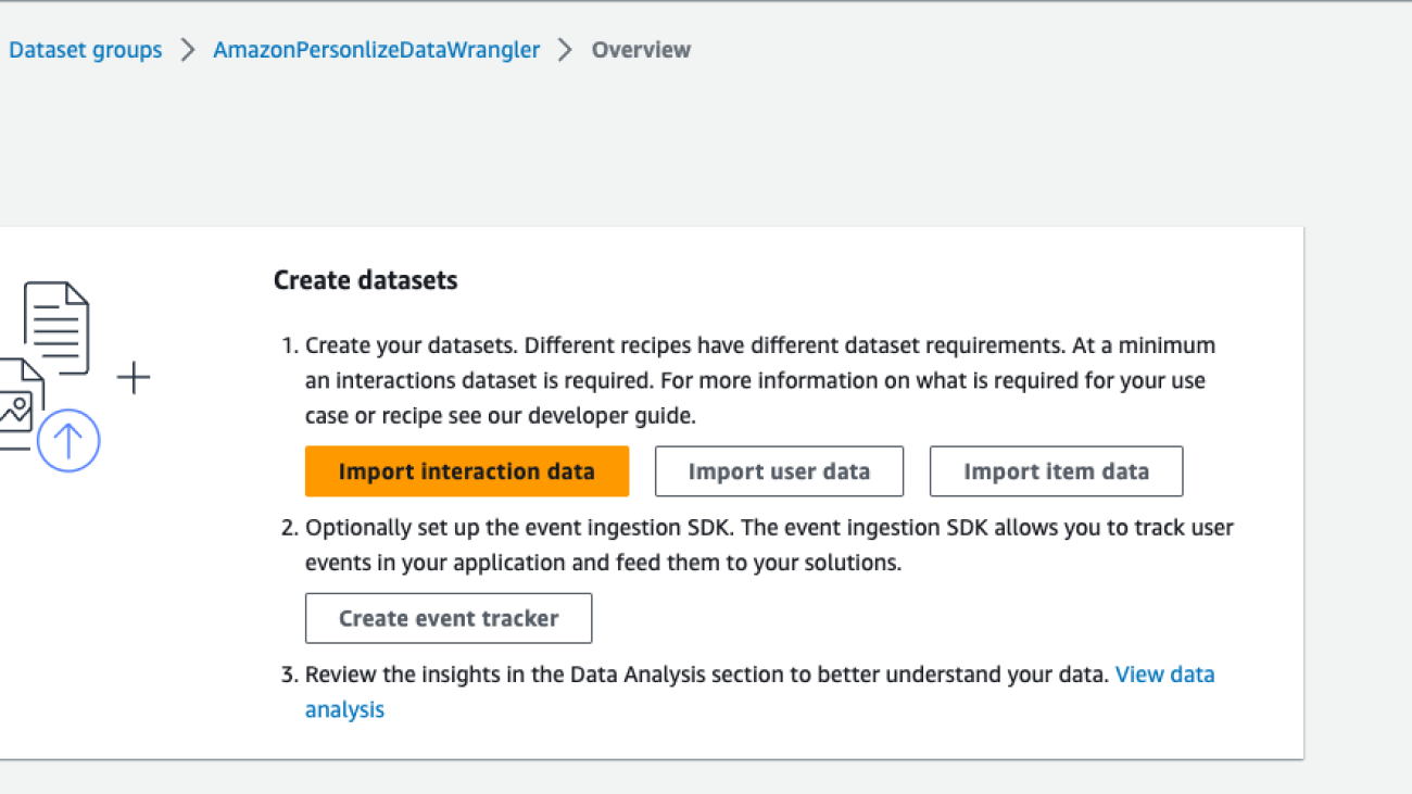
- On the Amazon Personalize console, navigate to the Overview page of your dataset group.
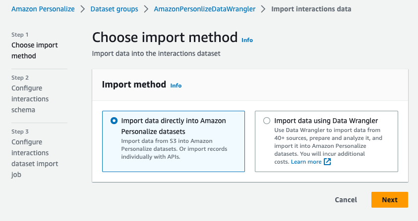
- Choose Import interaction data, Import user data, or Import item data, depending on the dataset type (for this post, we choose Import interaction data).

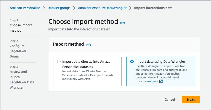
- For Import method, select Import data using Data Wrangler.
- Choose Next.
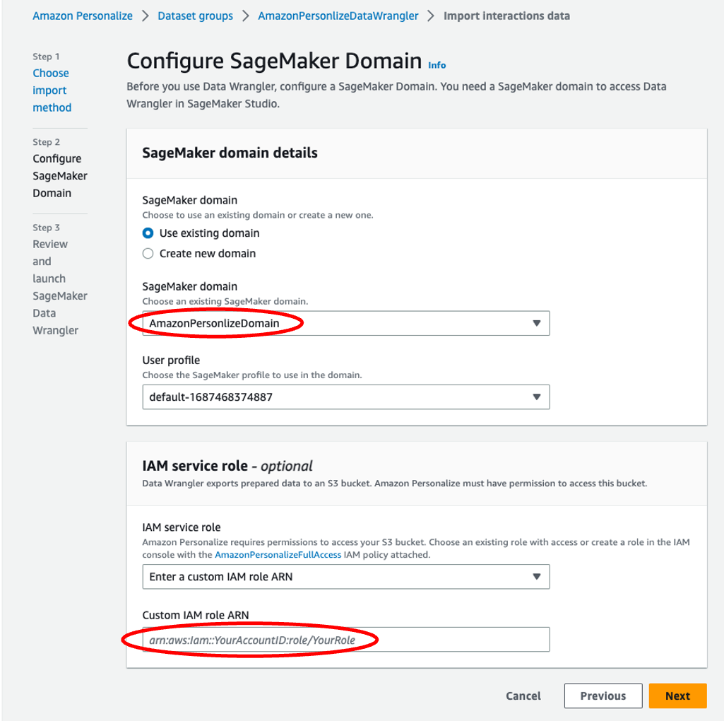
- Specify the SageMaker domain, user profile, and IAM service role that you created earlier as part of the prerequisites.
- Choose Next.
- Continue through the steps to launch an instance of SageMaker Data Wrangler.
Setting up the environment for the first time can take up to 5 minutes.
Import the raw data into SageMaker Data Wrangler
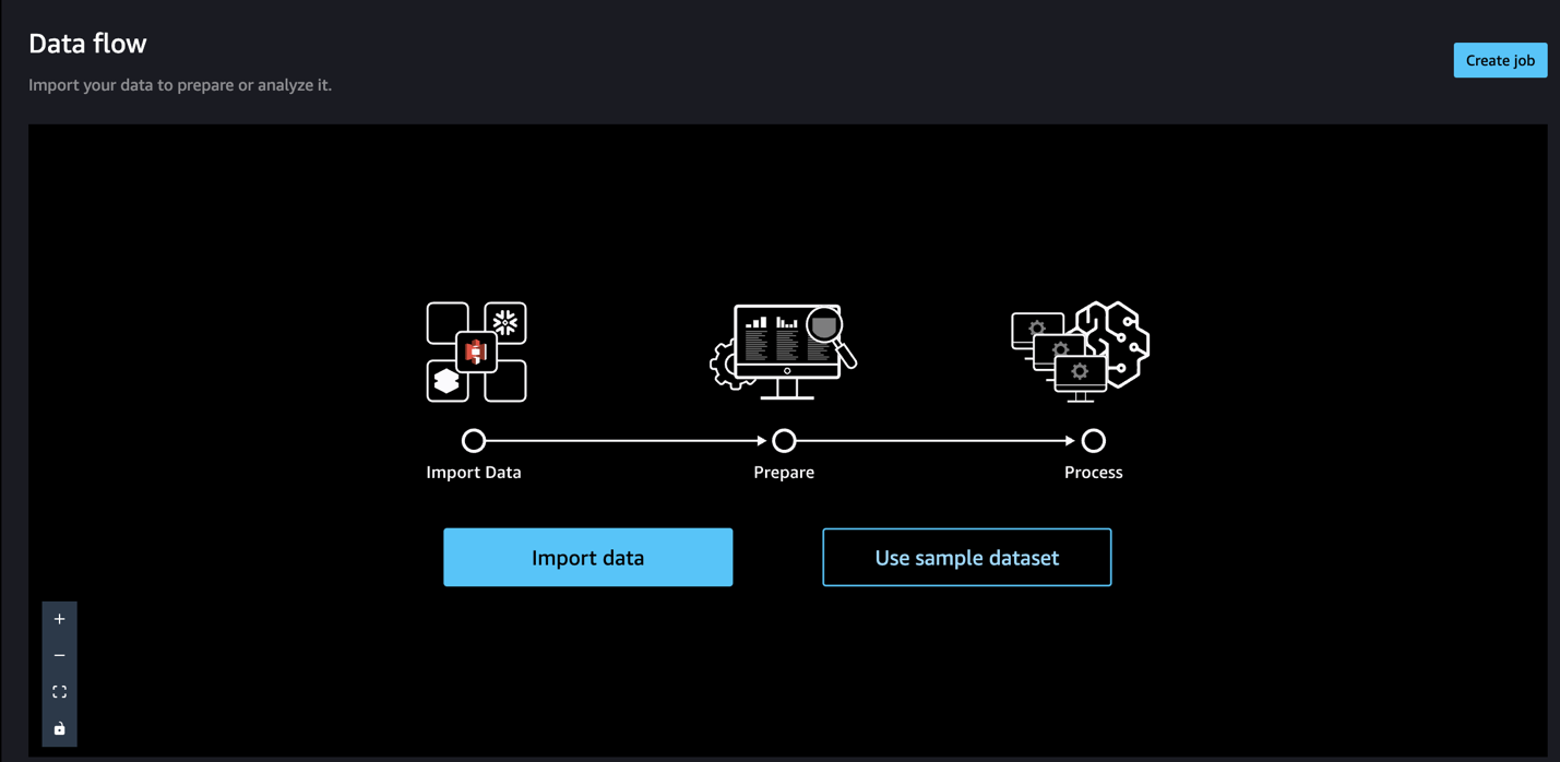
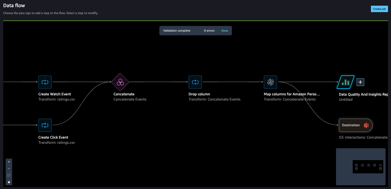
When using SageMaker Data Wrangler to prepare and import data, we use a data flow. A data flow defines a series of transformations and analyses on data to prepare it to create a machine learning model. Each time we add a step to our flow, SageMaker Data Wrangler takes an action on our data, such as joining it with another dataset or dropping some rows and columns.
To start, let’s import the raw data.
- On the data flow page, choose Import data.
With SageMaker Data Wrangler, we can import data from over 50 supported data sources.
- For Data sources¸ choose Amazon S3.
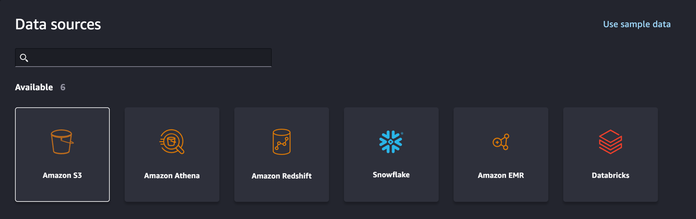
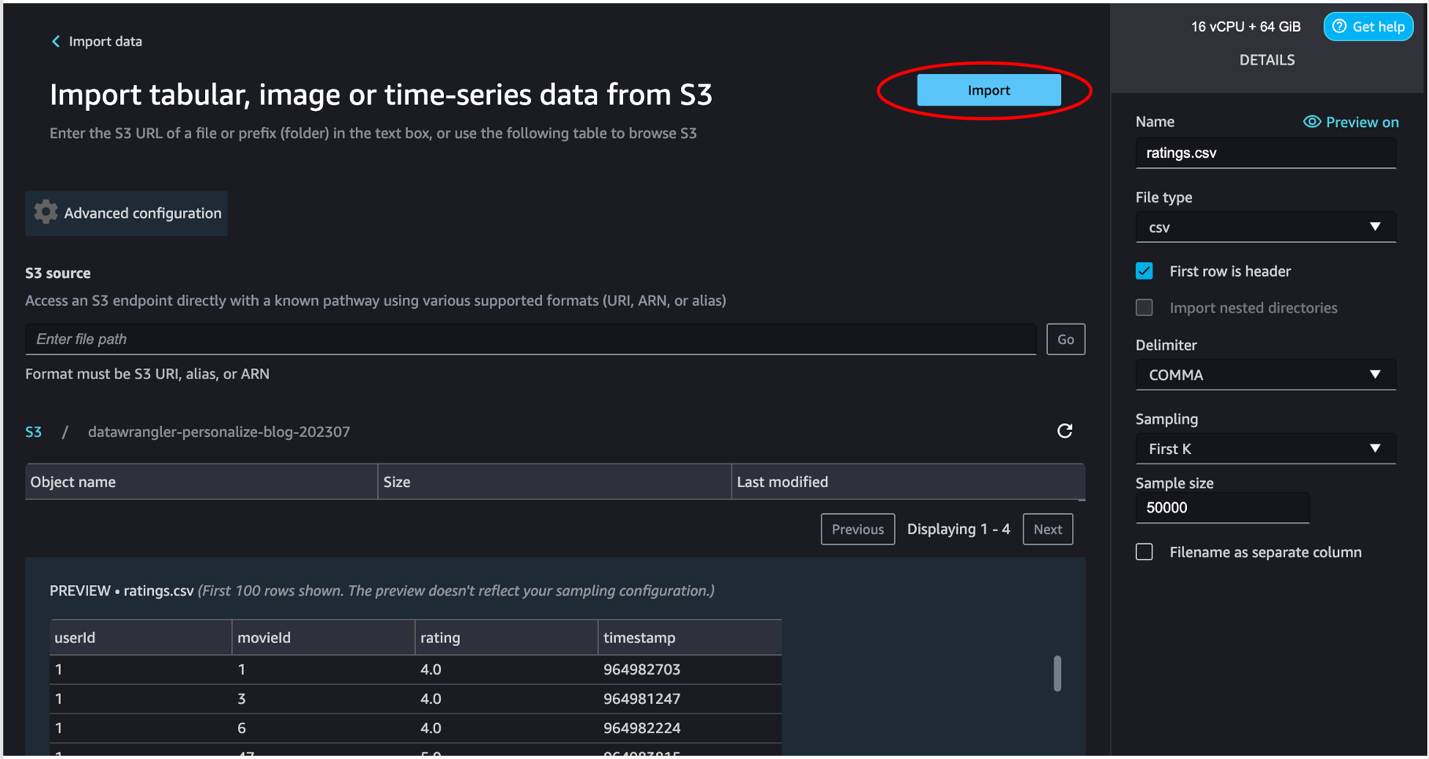
- Choose the dataset you uploaded to your S3 bucket.
SageMaker Data Wrangler automatically displays a preview of the data.
- Keep the default settings and choose Import.
After the data is imported, SageMaker Data Wrangler automatically validates the datasets and detects the data types for all the columns based on its sampling.
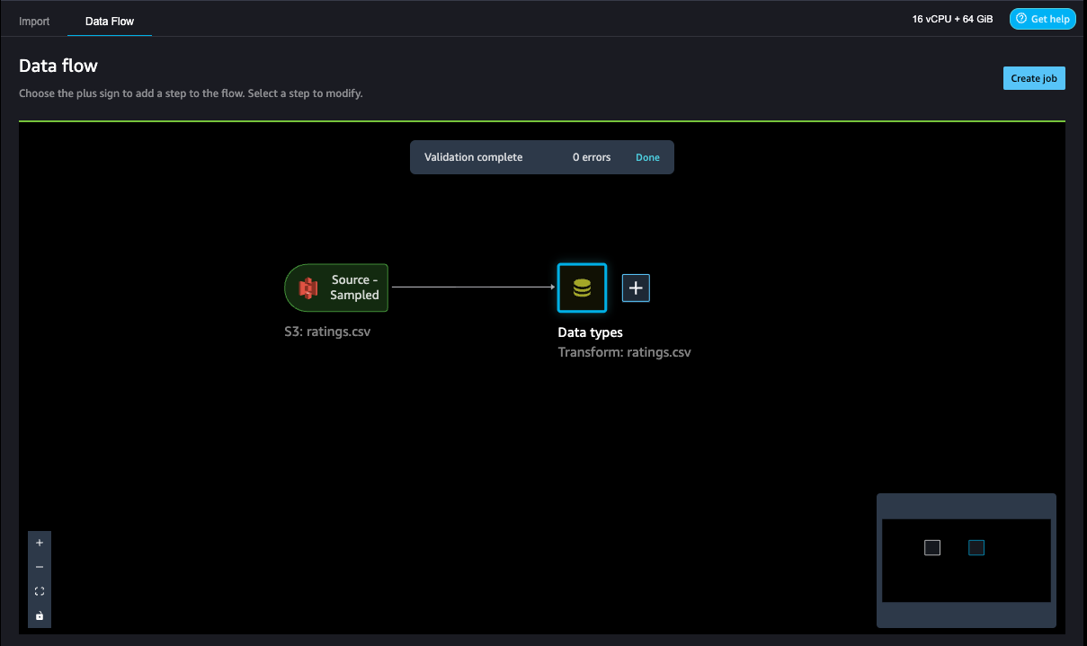
- Choose Data flow at the top of the Data types page to view the main data flow before moving to the next step.
One of the main advantages of SageMaker Data Wrangler is the ability to run previews of your transformations on a small subset of data before committing to apply the transformations on the entire dataset. To run the same transformation on multiple partitioned files in Amazon S3, you can use parameters.
Transform the data
To transform data in SageMaker Data Wrangler, you add a Transform step to your data flow. SageMaker Data Wrangler includes over 300 transforms that you can use to prepare your data, including a Map columns for Amazon Personalize transform. You can use the general SageMaker Data Wrangler transforms to fix issues such as outliers, type issues, and missing values, or apply data preprocessing steps.
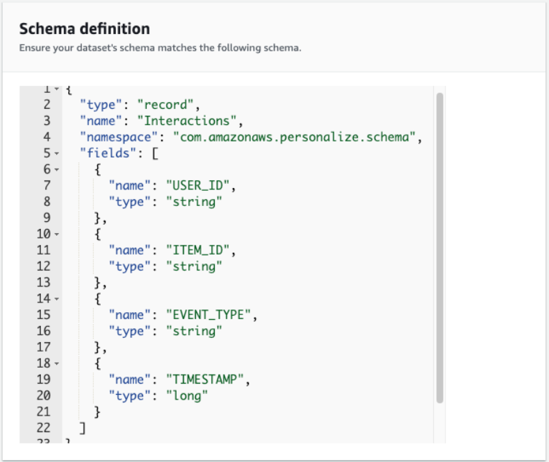
To use Amazon Personalize, the data you provided in the interactions dataset must match your dataset schema. For our movie recommender engine, the proposed interactions dataset schema includes:
user_id(string)item_id(string)event_type(string)timestamp(in Unix epoch time format)
To learn more about Amazon Personalize datasets and schemas, refer to Datasets and schemas.
The ratings.csv file as shown in the last step in the previous section includes movies rated from 1–5. We want to build a movie recommender engine based on that. To do so, we must complete the following steps:
- Modify the columns data types.
- Create two event types: Click and Watch.
- Assign all movies rated 2 and above as Click and movies rated 4 and above as both Click and Watch.
- Drop the
ratingscolumn. - Map the columns to the Amazon Personalize interactions dataset schema.
- Validate that our timestamp is in Unix epoch time.
Note that Step 3 isn’t needed to make a personalization model. If we want to use one of the Amazon Personalize streamlined video on demand domain recommenders, such as Top Picks for You, Click and Watch would be required event types. However, if we don’t have these, we could not include an event type field (or add our own event types such as the raw user ratings) and use a custom recipe such as User Personalization. Regardless of what type of recommendation engine we use, we need to ensure our dataset contains only representations of positive user intent. So whatever approach you choose, you need to drop all one-star ratings (and possibly two-star ratings as well).
Now let’s use SageMaker Data Wrangler to perform the preceding steps.
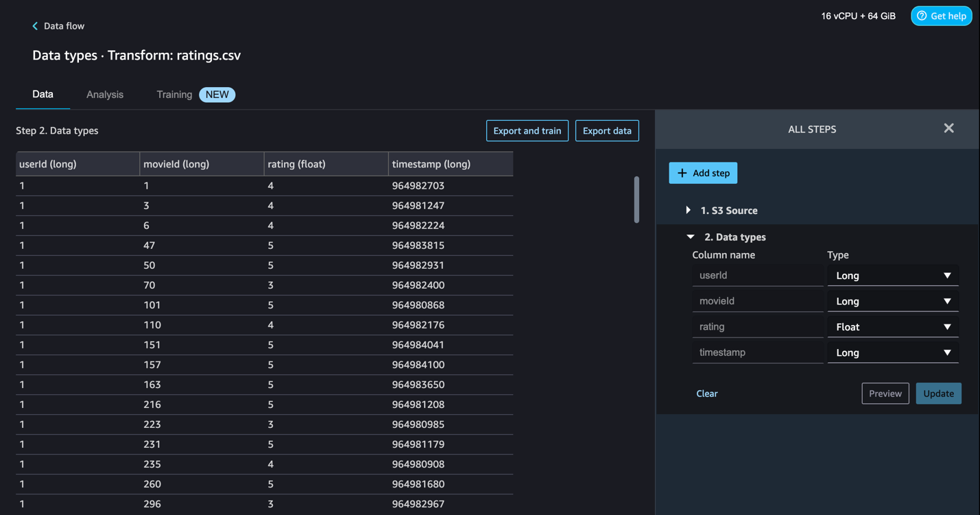
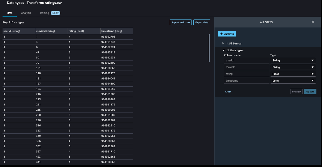
- On the Data flow page, choose the first transform, called Data types.
- Update the type for each column.
- Choose Preview to reflect the changes, then choose Update.
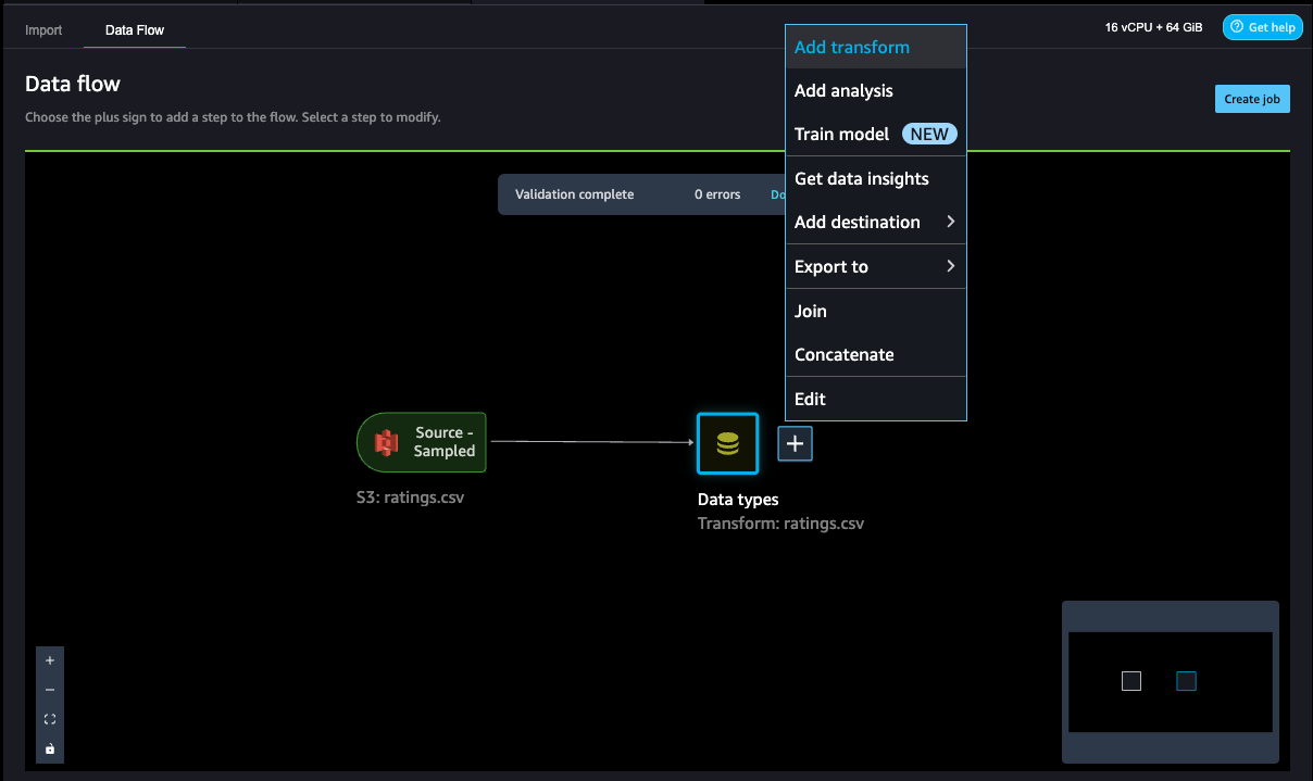
- To add a step in the data flow, choose the plus sign next to the step you want to perform the transform on, then choose Add transform.
- To filter the event Click out of the movie ratings, we add a Filter data step to filter out the movies rated 2 and above.
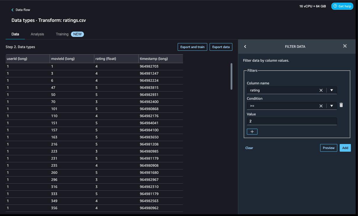
- Add another custom transform step to add a new column,
eventType, with Click as an assigned value. - Choose Preview to review your transformation to double-check the results are as intended, then choose Add.
- In this case, we write some PySpark code to add a column called
eventTypewhose value will be uniformly Click for all of our two-star through five-star movies:

- For the Watch events, repeat the previous steps for movies rated 4 and above and assign the Watch value by adding the steps to the Data types step. Our PySpark code for these steps is as follows:
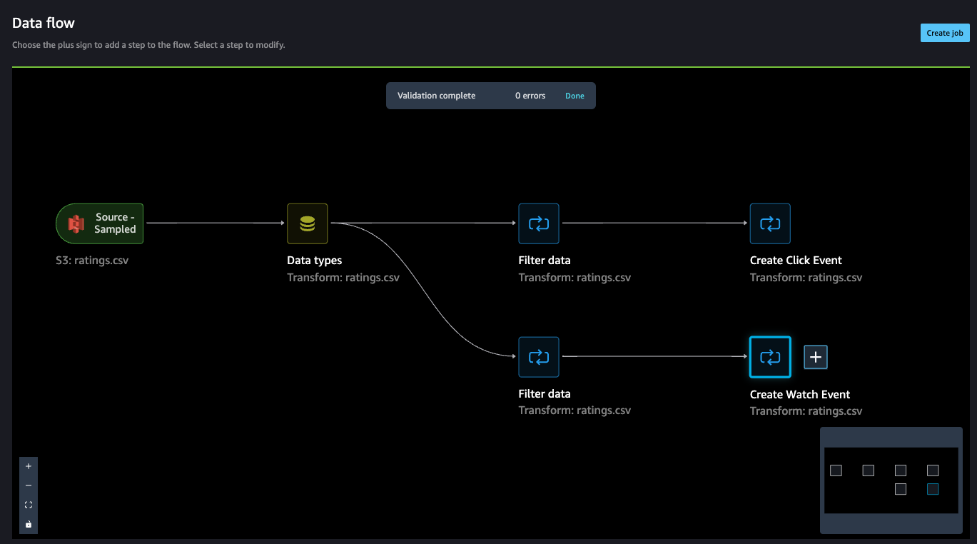
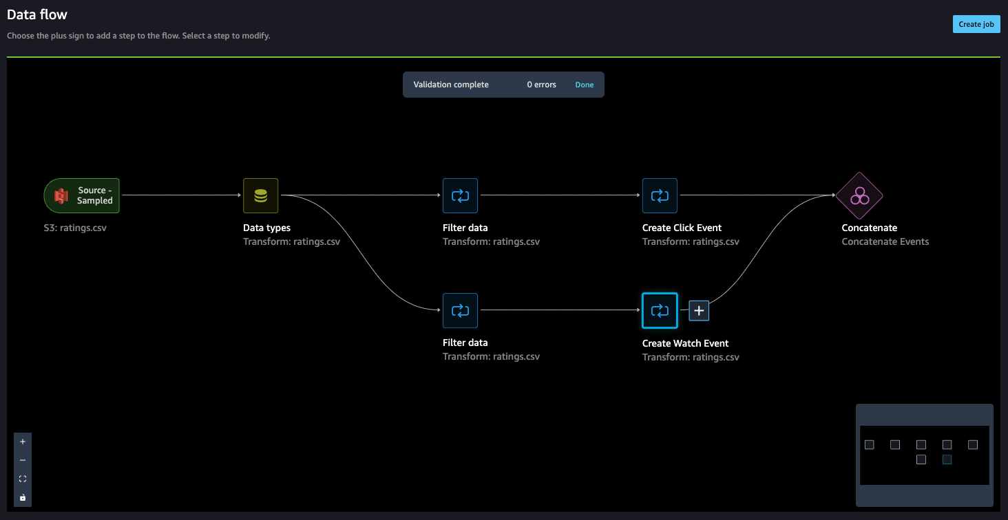
Up to this point, the data flow should look like the following screenshot.
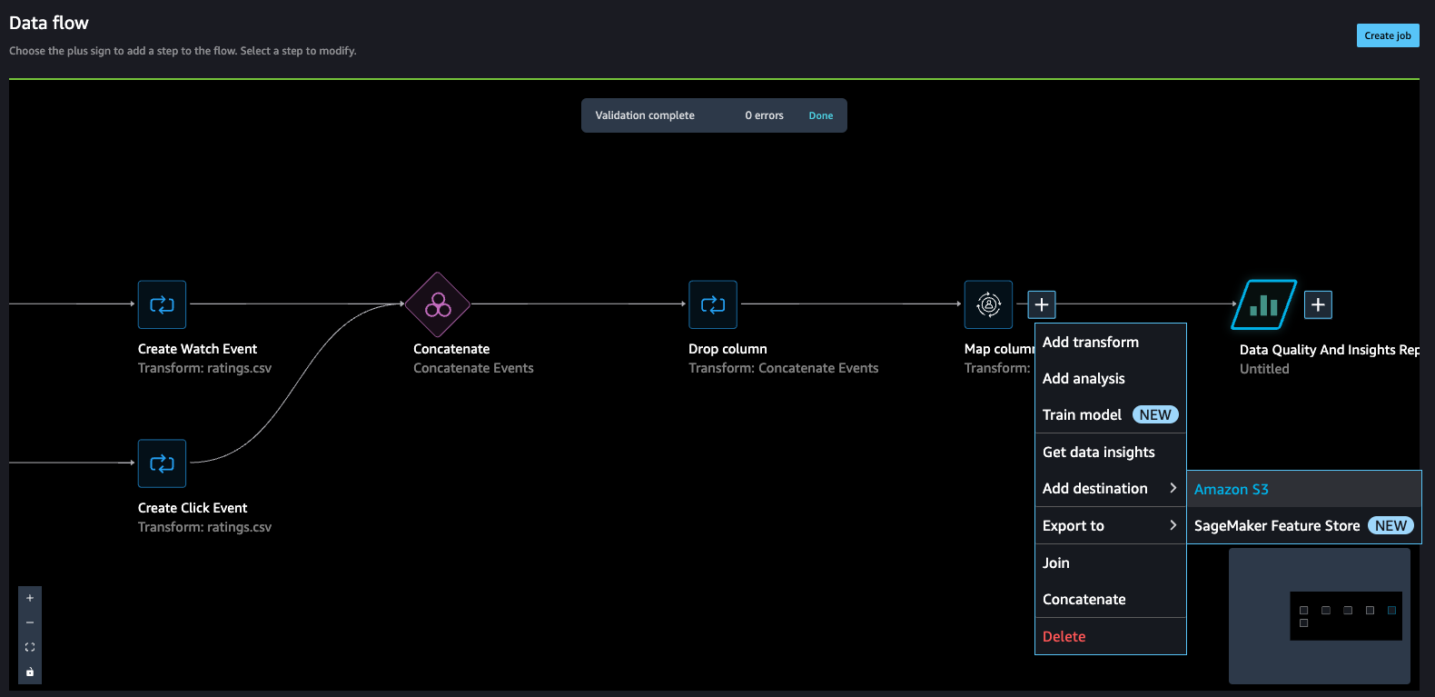
Concatenate datasets
Because we have two datasets for watched and clicked events, let’s walk through how to concatenate these into one interactions dataset.
- On the Data flow page, choose the plus sign next to Create Watch Event and choose Concatenate.
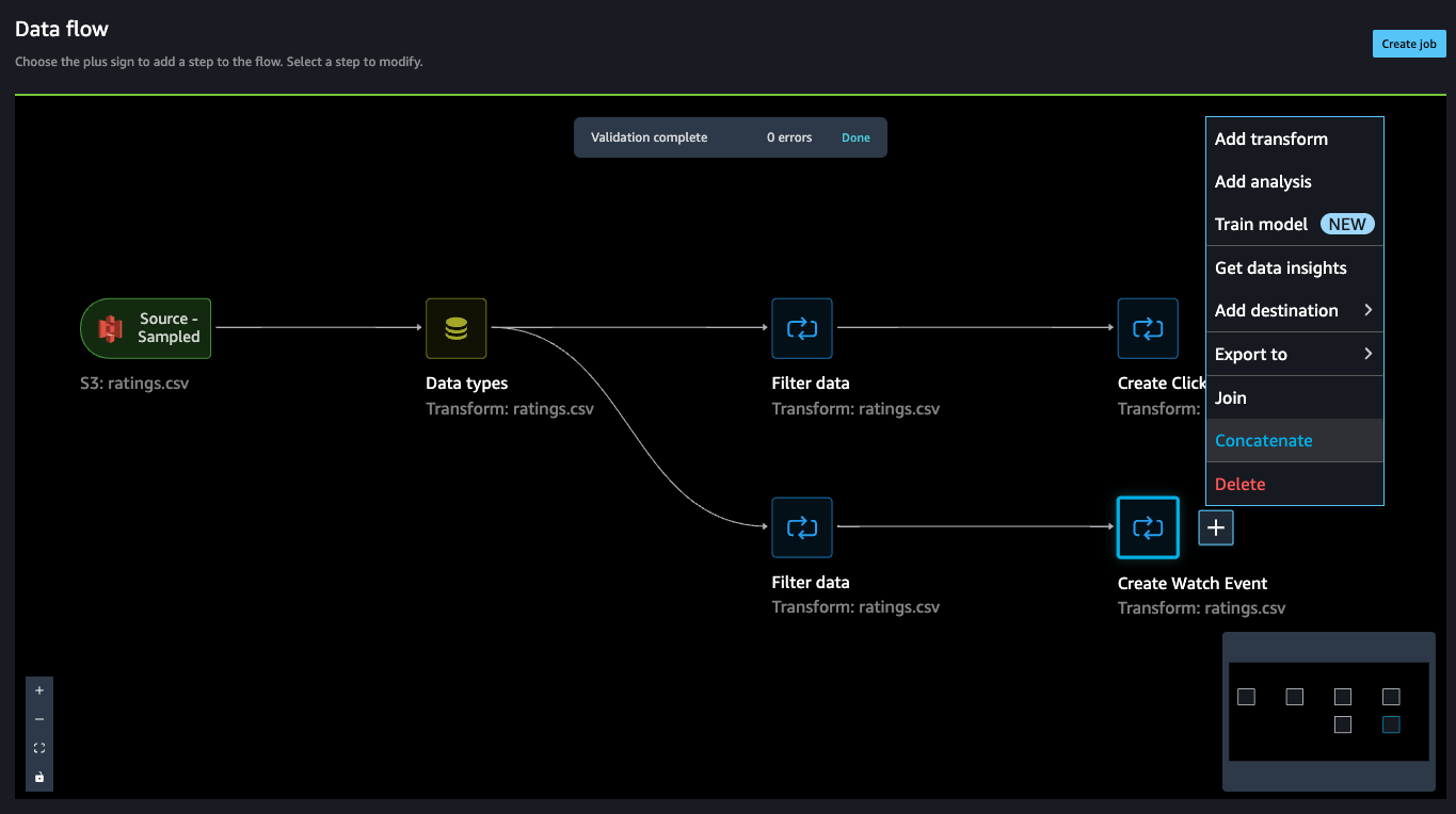
- Choose the other final step (Create Click Event), and this should automatically map (converge) both the sets into a concatenate preview.
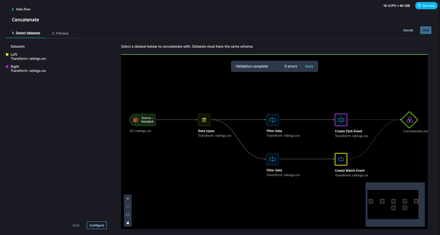
- Choose Configure to view a preview of the concatenated datasets.
- Add a name to the step.
- Choose Add to add the step.
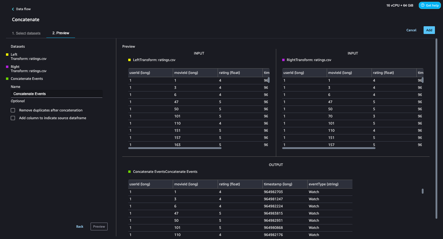
The data flow now looks like the following screenshot.
- Now, let’s add a Manage columns step to drop the original rating column.

Amazon Personalize has default column names for users, items, and timestamps. These default column names are user_id, item_id, and timestamp.
- Let’s add a Transform for Amazon Personalize step to replace the existing column headers with the default headers.
- In our case, we also use the
event_typefield, so let’s map that as well.
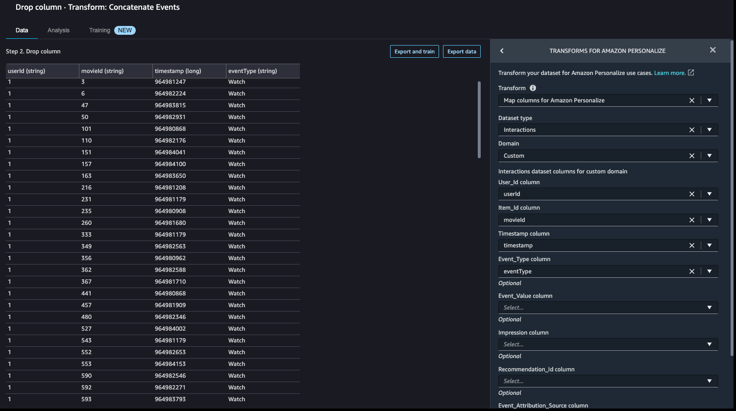
With this step, the data transformation activity is complete and the interactions dataset is ready for the next step.

Next, let’s validate our timestamps.
- We can do this by adding a Custom transform step. For this post, we choose Python (User-Defined Function).
- Choose timestamp as the input column and as the output, create a new column called
readable_timestamp. - Choose Python as the mode for the transformation and insert the following code for the Python function:
- Choose Preview to review the changes.

In this case, we see dates in the 2000s—because MovieLens started collecting data in 1996, this aligns with what is expected. If we don’t choose Add, this transformation won’t be added to our data flow.
- Because this was merely a sanity check, you can navigate back to the data flow by choosing Data flow in the upper left corner.

Finally, we add an analysis step to create a summary report about the dataset. This step performs an analysis to assess the suitability of the dataset for Amazon Personalize.
- Choose the plus sign next to the final step on the data flow and choose Add analysis.
- For Analysis type¸ choose Data Quality And Insights Report for Amazon Personalize.
- For Dataset type¸ choose Interactions.
- Choose Create.
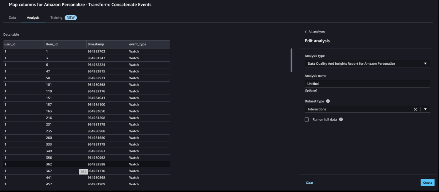
The MovieLens dataset is quite clean, so the analysis shows no issues. If some issues were identified, you can iterate on the dataset and rerun the analysis until you can address them.
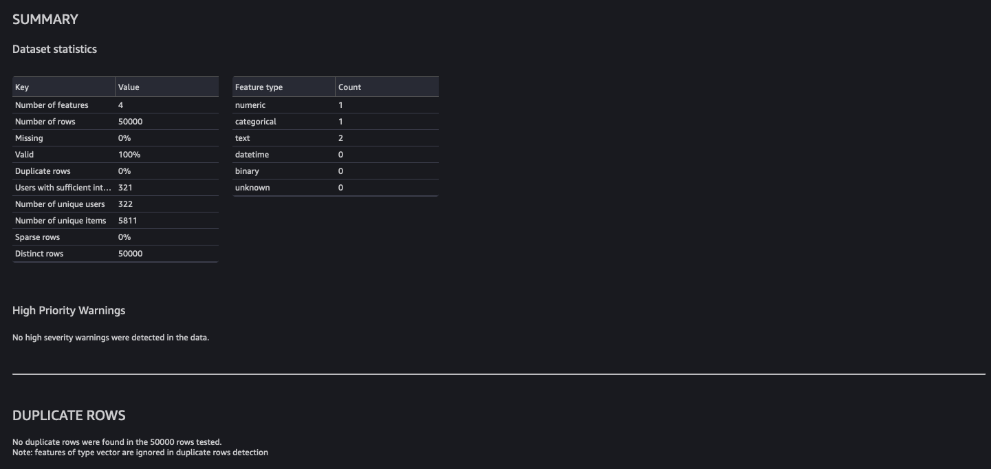
Note the analysis by default runs on a sample of 50,000 rows.
Import the dataset to Amazon Personalize
At this point, our raw data has been transformed and we are ready to import the transformed interactions dataset to Amazon Personalize. SageMaker Data Wrangler gives you the ability to export your data to a location within an S3 bucket. You can specify the location using one of the following methods:
- Destination node – Where SageMaker Data Wrangler stores the data after it has processed it
- Export to – Exports the data resulting from a transformation to Amazon S3
- Export data – For small datasets, you can quickly export the data that you’ve transformed
With the Destination node method, to export your data, you create destination nodes and a SageMaker Data Wrangler job. Creating a SageMaker Data Wrangler job starts a SageMaker Processing job to export your flow. You can choose the destination nodes that you want to export after you’ve created them.
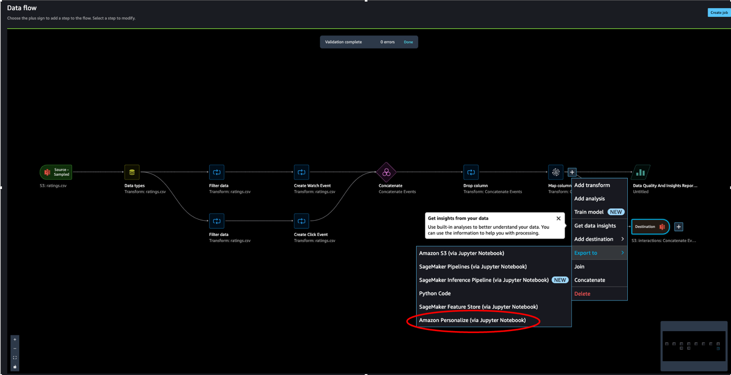
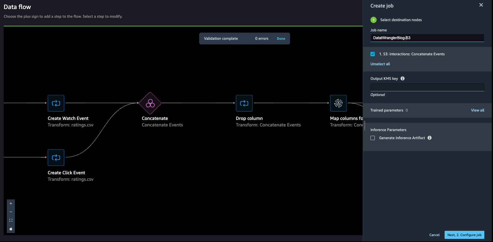
- Choose the plus sign next to the node that represents the transformations you want to export.
- Choose Export to and then choose Amazon S3 (via Jupyter Notebook).
Note we could have also chosen to export the data to Amazon Personalize via a Jupyter notebook available in SageMaker Data Wrangler.
- For Dataset name, enter a name, which will be used as a folder name in the S3 bucket provided as a destination.
- You can specify the file type, field delimiter, and compression method.
- Optionally, specify the number of partitions and column to partition by.
- Choose Add destination.
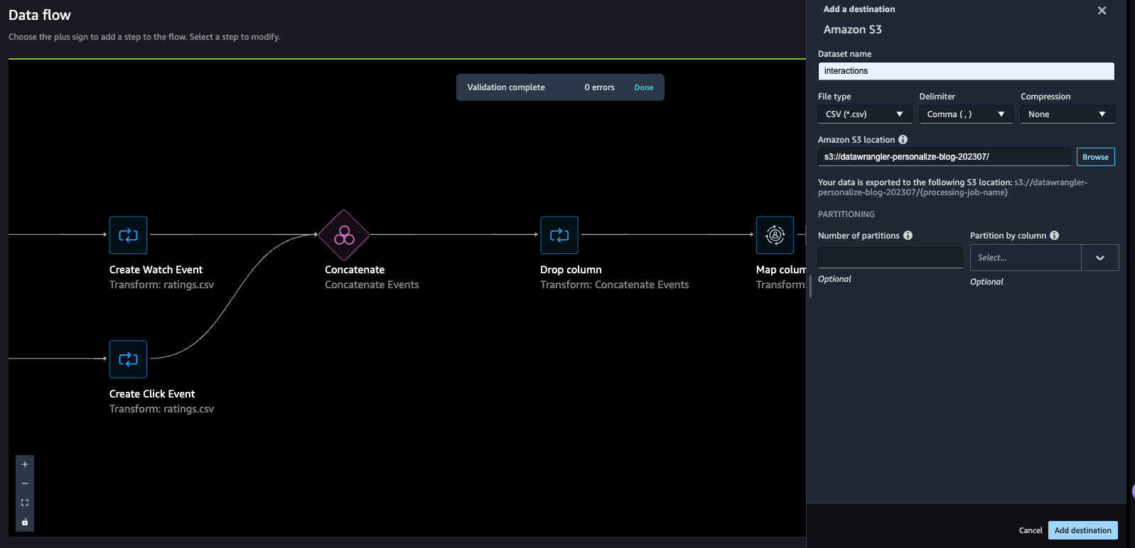
The data flow should look like the following screenshot.
- Create a job to process the data flow and store the data in the destination (S3 bucket) that we configured in the previous step.
- Enter a job name, then choose Configure job.
SageMaker Data Wrangler provides the ability to configure the instance type, instance count, and job configuration, and the ability to create a schedule to process the job. For guidance on how to choose an instance count, refer to Create and Use a Data Wrangler Flow.
To monitor the status of the job, navigate to the Dashboard page on the SageMaker console. The Processing section shows the number of completed and created jobs. You can drill down to get more details about the completed job.
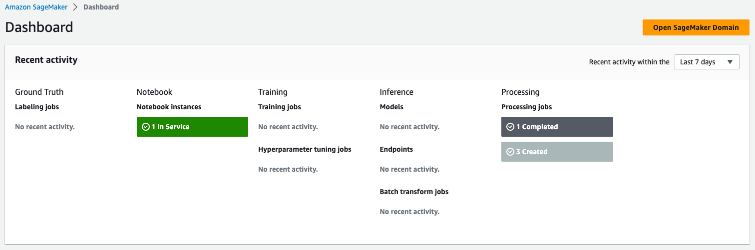
When the job is complete, a new file of the transformed data is created in the destination specified.
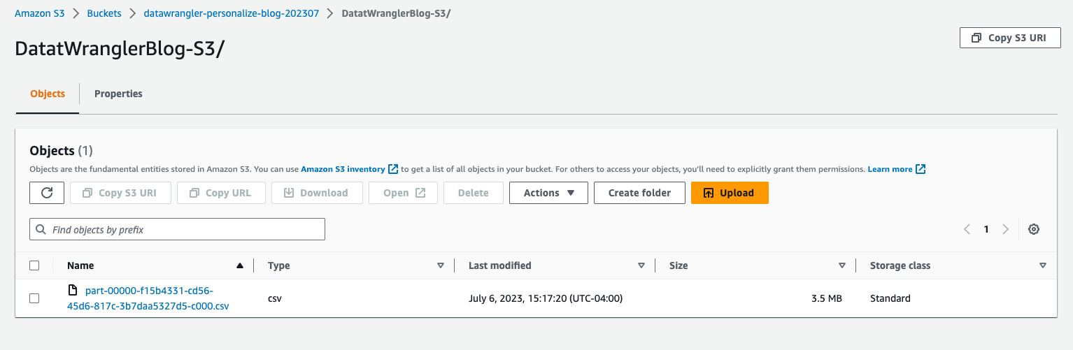
- Return to the Amazon Personalize console and navigate to the dataset group to import another dataset.
- Choose Import interaction data.

- Select Import data directly into Amazon Personalize datasets to import the transformed dataset directly from Amazon S3, then choose Next.
- Define the schema. For this post, our case our dataset consists of the
user_id(string),item_id(string),event_type(string), andtimestamp(long) fields.
At this point, you can create a video on demand domain recommender or a custom solution. To do so, follow the steps in Preparing and importing data
Conclusion
In this post, we described how to use SageMaker Data Wrangler to prepare a sample dataset for Amazon Personalize. SageMaker Data Wrangler offers over 300 transformations. These transformations and the ability to add custom user transformations can help streamline the process of creating a quality dataset to offer hyper-personalized content to end-users.
Although we only explored how to prepare an interactions dataset in this post, you can use SageMaker Data Wrangler to prepare user and item datasets as well. For more information on the types of data that can be used with Amazon Personalize, refer to Datasets and schemas.
If you’re new to Amazon Personalize or SageMaker Data Wrangler, refer to Get Started with Amazon Personalize or Get Started with SageMaker Data Wrangler, respectively. If you have any questions related to this post, please add them in the comments section.
About the Authors
 Maysara Hamdan is a Partner Solutions Architect based in Atlanta, Georgia. Maysara has over 15 years of experience in building and architecting Software Applications and IoT Connected Products in Telecom and Automotive Industries. In AWS, Maysara helps partners in building their cloud practices and growing their businesses. Maysara is passionate about new technologies and is always looking for ways to help partners innovate and grow.
 Eric Bolme is a Specialist Solution Architect with AWS based on the East Coast of the United States. He has 8 years of experience building out a variety of deep learning and other AI use cases and focuses on Personalization and Recommendation use cases with AWS.