October 2023 – Page 16

New contrastive-learning methods for better data representation

New loss functions enable better approximation of the optimal loss and more-useful representations of multimodal data.Read More

Scalable spherical CNNs for scientific applications

Posted by Carlos Esteves and Ameesh Makadia, Research Scientists, Google Research, Athena Team

Typical deep learning models for computer vision, like convolutional neural networks (CNNs) and vision transformers (ViT), process signals assuming planar (flat) spaces. For example, digital images are represented as a grid of pixels on a plane. However, this type of data makes up only a fraction of the data we encounter in scientific applications. Variables sampled from the Earth’s atmosphere, like temperature and humidity, are naturally represented on the sphere. Some kinds of cosmological data and panoramic photos are also spherical signals, and are better treated as such.

Using methods designed for planar images to process spherical signals is problematic for a couple of reasons. First, there is a sampling problem, i.e., there is no way of defining uniform grids on the sphere, which are needed for planar CNNs and ViTs, without heavy distortion.

When projecting the sphere into a plane, the patch represented by the red circle is heavily distorted near the poles. This sampling problem hurts the accuracy of conventional CNNs and ViTs on spherical inputs.

Second, signals and local patterns on the sphere are often complicated by rotations, so models need a way to address that. We would like equivariance to 3D rotations, which ensures that learned features follow the rotations of the input. This leads to better utilization of the model parameters and allows training with less data. Equivariance to 3D rotations is also useful in most settings where inputs don’t have a preferred orientation, such as 3D shapes and molecules.

Drone racing with panoramic cameras. Here the sharp turns result in large 3D rotations of the spherical image. We would like our models to be robust to such rotations. Source: https://www.youtube.com/watch?v=_J7qXbbXY80 (licensed under CC BY)

In the atmosphere, it is common to see similar patterns appearing at different positions and orientations. We would like our models to share parameters to recognize these patterns.

With the above challenges in mind, in “Scaling Spherical CNNs”, presented at ICML 2023, we introduce an open-source library in JAX for deep learning on spherical surfaces. We demonstrate how applications of this library match or surpass state-of-the-art performance on weather forecasting and molecular property prediction benchmarks, tasks that are typically addressed with transformers and graph neural networks.

Background on spherical CNNs

Spherical CNNs solve both the problems of sampling and of robustness to rotation by leveraging spherical convolution and cross-correlation operations, which are typically computed via generalized Fourier transforms. For planar surfaces, however, convolution with small filters is faster, because it can be performed on regular grids without using Fourier transforms. The higher computational cost for spherical inputs has so far restricted the application of spherical CNNs to small models and datasets and low resolution datasets.

Our contributions

We have implemented the spherical convolutions from spin-weighted spherical CNNs in JAX with a focus on speed, and have enabled distributed training over a large number of TPUs using data parallelism. We also introduced a new phase collapse activation and spectral batch normalization layer, and a new residual block that improves accuracy and efficiency, which allows training more accurate models up to 100x larger than before. We apply these new models on molecular property regression and weather forecasting.

We scale spherical CNNs by up to two orders of magnitude in terms of feature sizes and model capacity, compared to the literature: Cohen’18, Esteves’18, Esteves’20, and Cobb’21. VGG-19 is included as a conventional CNN reference. Our largest model for weather forecasting has 256 x 256 x 78 inputs and outputs, and runs 96 convolutional layers during training with a lowest internal resolution of 128 x 128 x 256.

Molecular property regression

Predicting properties of molecules has applications in drug discovery, where the goal is to quickly screen numerous molecules in search of those with desirable properties. Similar models may also be relevant in the design of drugs targeting the interaction between proteins. Current methods in computational or experimental quantum chemistry are expensive, which motivates the use of machine learning.

Molecules can be represented by a set of atoms and their positions in 3D space; rotations of the molecule change the positions but not the molecular properties. This motivates the application of spherical CNNs because of their rotation equivariance. However, molecules are not defined as signals on the sphere so the first step is to map them to a set of spherical functions. We do so by leveraging physics-based interactions between the atoms of the molecule.

Each atom is represented by a set of spherical signals accumulating physical interactions with other atoms of each type (shown in the three panels on the right). For example, the oxygen atom (O; top panel) has a channel for oxygen (indicated by the sphere labeled “O” on the left) and hydrogen (“H”, right). The accumulated Coulomb forces on the oxygen atom with respect to the two hydrogen atoms is indicated by the red shaded regions on the bottom of the sphere labeled “H”. Because the oxygen atom contributes no forces to itself, the “O” sphere is uniform. We include extra channels for the Van der Waals forces.

Spherical CNNs are applied to each atom’s features, and results are later combined to produce the property predictions. This results in state-of-the art performance in most properties as typically evaluated in the QM9 benchmark:

Error comparison against the state-of-the-art on 12 properties of QM9 (see the dataset paper for details). We show TorchMD-Net and PaiNN results, normalizing TorchMD-Net errors to 1.0 (lower is better). Our model, shown in green, outperforms the baselines in most targets.

Weather forecasting

Accurate climate forecasts serve as invaluable tools for providing timely warnings of extreme weather events, enabling effective water resource management, and guiding informed infrastructure planning. In a world increasingly threatened by climate disasters, there is an urgency to deliver forecasts much faster and more accurately over a longer time horizon than general circulation models. Forecasting models will also be important for predicting the safety and effectiveness of efforts intended to combat climate change, such as climate interventions. The current state-of-the-art uses costly numerical models based on fluid dynamics and thermodynamics, which tend to drift after a few days.

Given these challenges, there is an urgency for machine learning researchers to address climate forecasting problems, as data-driven techniques have the potential of both reducing the computational cost and improving long range accuracy. Spherical CNNs are suitable for this task since atmospheric data is natively presented on the sphere. They can also efficiently handle repeating patterns at different positions and orientations that are common in such data.

We apply our models to several weather forecasting benchmarks and outperform or match neural weather models based on conventional CNNs (specifically, 1, 2, and 3). Below we show results in a test setting where the model takes a number of atmospheric variables as input and predicts their values six hours ahead. The model is then iteratively applied on its own predictions to produce longer forecasts. During training, the model predicts up to three days ahead, and is evaluated up to five days. Keisler proposed a graph neural network for this task, but we show that spherical CNNs can match the GNN accuracy in the same setting.

Iterative weather forecasting up to five days (120h) ahead with spherical CNNs. The animations show the specific humidity forecast at a given pressure and its error.

Wind speed and temperature forecasts with spherical CNNs.

Additional resources

Our JAX library for efficient spherical CNNs is now available. We have shown applications to molecular property regression and weather forecasting, and we believe the library will be helpful in other scientific applications, as well as in computer vision and 3D vision.

Weather forecasting is an active area of research at Google with the goal of building more accurate and robust models — like Graphcast, a recent ML-based mid-range forecasting model — and to build tools that enable further advancement across the research community, such as the recently released WeatherBench 2.

Acknowledgements

This work was done in collaboration with Jean-Jacques Slotine, and is based on previous collaborations with Kostas Daniilidis and Christine Allen-Blanchette. We thank Stephan Hoyer, Stephan Rasp, and Ignacio Lopez-Gomez for helping with data processing and evaluation, and Fei Sha, Vivian Yang, Anudhyan Boral, Leonardo Zepeda-Núñez, and Avram Hershko for suggestions and discussions. We are thankful to Michael Riley and Corinna Cortes for supporting and encouraging this project.

How AI Helps Fight Wildfires in California

California has a new weapon against the wildfires that have devastated the state: AI.

A freshly launched system powered by AI trained on NVIDIA GPUs promises to provide timely alerts to first responders across the Golden State every time a blaze ignites.

The ALERTCalifornia initiative, a collaboration between California’s wildfire fighting agency CAL FIRE and the University of California, San Diego, uses advanced AI developed by DigitalPath.

Harnessing the raw power of NVIDIA GPUs and aided by a network of thousands of cameras dotting the Californian landscape, DigitalPath has refined a convolutional neural network to spot signs of fire in real time.

A Mission That’s Close to Home

DigitalPath CEO Jim Higgins said it’s a mission that means a lot to the 100-strong technology partner, which is nestled in the Sierra Nevada foothills in Chico, Calif., a short drive from the town of Paradise, where the state’s deadliest wildfire killed 85 people in 2018.

“It’s one of the main reasons we’re doing this,” Higgins said of the wildfire, the deadliest and most destructive in the history of the most populous U.S. state. “We don’t want people to lose their lives.”

The ALERTCalifornia initiative is based at UC San Diego’s Jacobs School of Engineering, the Qualcomm Institute and the Scripps Institution of Oceanography.

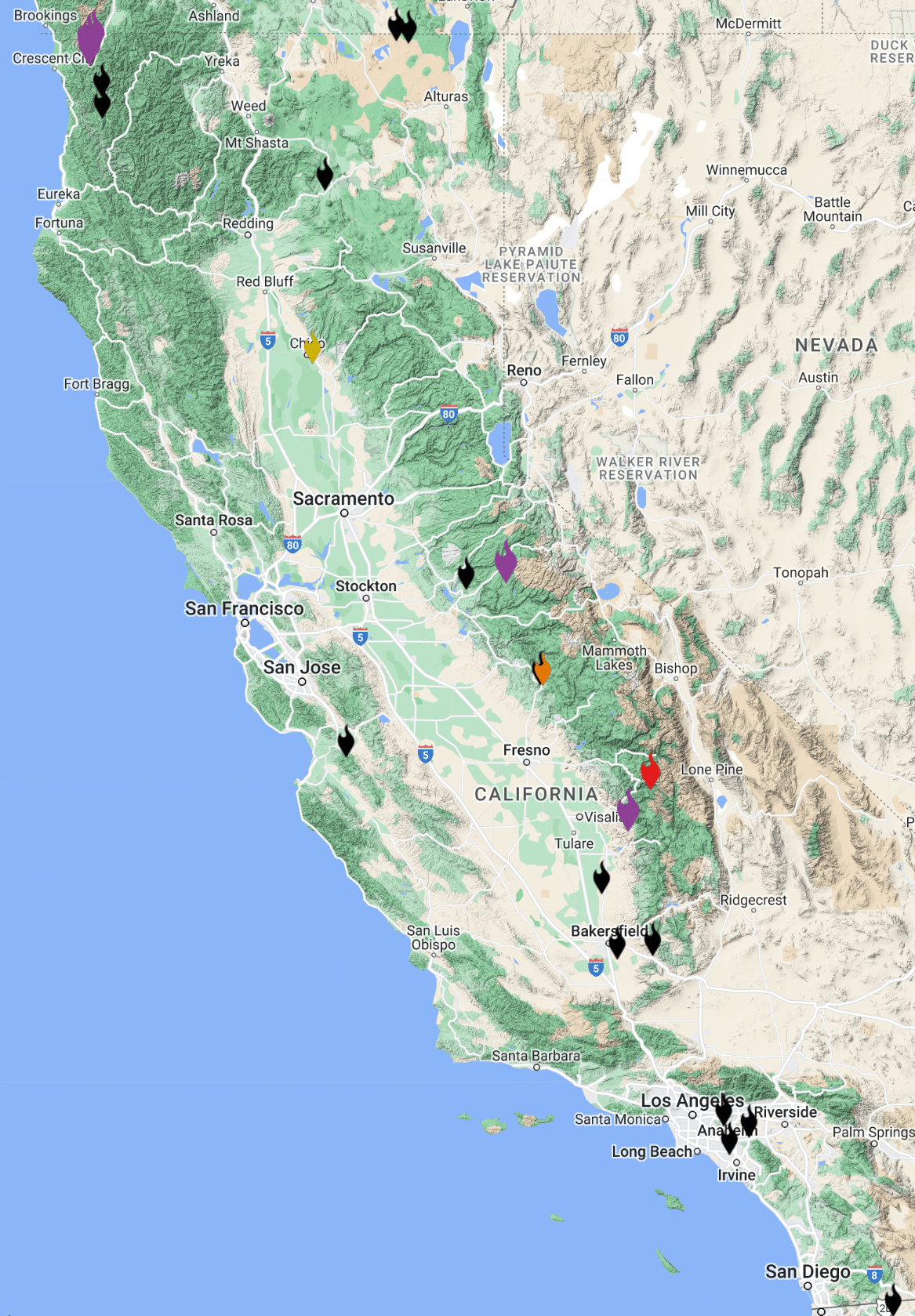
The program manages a network of thousands of monitoring cameras and sensor arrays and collects data that provides actionable, real-time information to inform public safety.

The AI program started in June and was initially deployed in six of Cal Fire’s command centers. This month it expanded to all of CAL FIRE’s 21 command centers.

ALERTCalifornia, powered by DigitalPath, can detect fires from cameras positioned across the golden state.

DigitalPath began by building out a management platform for a network of cameras used to confirm California wildfires after a 911 call.

The company quickly realized there would be no way to have people examine images from the thousands of cameras relaying images to the system every ten to fifteen seconds.

So Ethan Higgins, the company’s system architect, turned to AI.

The team began by training a convolutional neural network on a cloud-based system running an NVIDIA A100 Tensor Core GPU and later transitioned to a system running on eight A100 GPUs.

The AI model is crucial to examining a system that sees almost 8 million images a day streaming in from over 1,000 first-party cameras, primarily in California, and thousands more from third-party sources nationwide, he said.

Impact of Wildfires

All anomalies being tracked throughout California as of Sept. 20, 2023. Image Credit: DigitalPath

It’s arriving just in time.

Wildfires have ravaged California over the past decade, burning millions of acres of land, destroying thousands of homes and businesses and claiming hundreds of lives.

According to CAL FIRE, in 2020 alone, the state experienced five of its six largest and seven of its 20 most destructive wildfires.

And the total dollar damage of wildfires in California from 2019 to 2021 was estimated at over $25 billion.

The new system promises to give first responders a crucial tool to prevent such conflagrations.

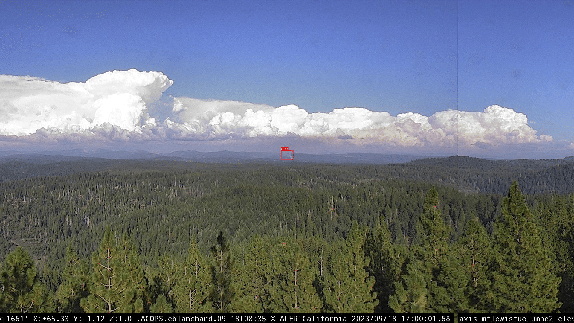
In fact, during a recent interview with DigitalPath, the system detected two separate fires in Northern California as they ignited.

Every day, the system detects between 50 and 300 events, offering invaluable real-time information to local first responders.

Beyond Detection: Enhancing Capabilities

Example of multiple cameras detecting a single anomaly. Image Credit: DigitalPath.

But AI is just part of the story.

The system is also a case study in how innovative companies can use AI to amplify their unique capabilities.

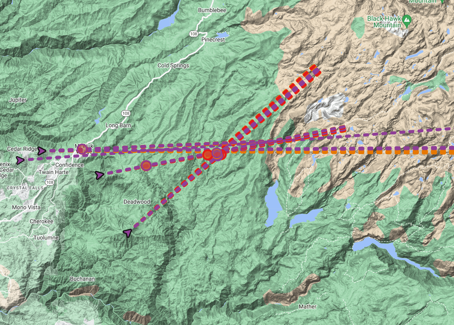
One of DigitalPath’s breakthroughs is its system’s ability to identify the same fire captured from diverse camera angles. DigitalPath’s system efficiently filters imagery down to a human-digestible level. The system filters 8 million daily images down to just 100 alerts, or 1.25 thousandths of one percent of total images captured.

“The system was designed from the start with human processing in mind,” Higgins said, ensuring that authorities receive a single, consolidated notification for every incident.

“We’ve got to catch every fire we can,” he adds.

Expanding Horizons

DigitalPath eventually hopes to expand its detection technology to help California detect more kinds of natural disasters.

And having proven its worth in California, DigitalPath is now in talks with state and county officials and university research teams across the fire-prone Western United States under its ALERTWest subsidiary.

Their goal: to help partners replicate the success of UC San Diego and ALERTCalifornia, potentially shielding countless lives and homes from the wrath of wildfires.

Featured image credit: SLworking2, via Flickr, Creative Commons license, some rights reserved.

Android 14: More customization, control and accessibility features

Android 14 is here with personal, protective and accessible features that put users first and celebrate their individuality.Read More

New Library Updates in PyTorch 2.1

Summary

We are bringing a number of improvements to the current PyTorch libraries, alongside the PyTorch 2.1 release. These updates demonstrate our focus on developing common and extensible APIs across all domains to make it easier for our community to build ecosystem projects on PyTorch.

Along with 2.1, we are also releasing a series of beta updates to the PyTorch domain libraries including TorchAudio and TorchVision. Please find the list of the latest stable versions and updates below.

Latest Stable Library Versions	(Full List)*
TorchArrow 0.1.0	TorchRec 0.4.0	TorchVision 0.16
TorchAudio 2.1	TorchServe 0.7.1	TorchX 0.5.0
TorchData 0.7.0	TorchText 0.16.0	PyTorch on XLA Devices 1.14

*To see prior versions or (unstable) nightlies, click on versions in the top left menu above ‘Search Docs’.

TorchAudio

TorchAudio v2.1 introduces the following new features and backward-incompatible changes:

[Beta] A new API to apply filter, effects and codec

`torchaudio.io.AudioEffector` can apply filters, effects and encodings to waveforms in online/offline fashion. You can use it as a form of augmentation.

Please refer to https://pytorch.org/audio/2.1/tutorials/effector_tutorial.html for the usage and examples.

[Beta] Tools for Forced alignment

New functions and a pre-trained model for forced alignment were added. `torchaudio.functional.forced_align` computes alignment from an emission and `torchaudio.pipelines.MMS_FA` provides access to the model trained for multilingual forced alignment in MMS: Scaling Speech Technology to 1000+ languages project.

Please refer to https://pytorch.org/audio/2.1/tutorials/ctc_forced_alignment_api_tutorial.html for the usage of `forced_align` function, and https://pytorch.org/audio/2.1/tutorials/forced_alignment_for_multilingual_data_tutorial.html for how one can use `MMS_FA` to align transcript in multiple languages.

[Beta] TorchAudio-Squim : Models for reference-free speech assessment

Model architectures and pre-trained models from the paper TorchAudio-Sequim: Reference-less Speech Quality and Intelligibility measures in TorchAudio were added.

You can use the pre-trained models `torchaudio.pipelines.SQUIM_SUBJECTIVE` and `torchaudio.pipelines.SQUIM_OBJECTIVE`. They can estimate the various speech quality and intelligibility metrics (e.g. STOI, wideband PESQ, Si-SDR, and MOS). This is helpful when evaluating the quality of speech generation models, such as Text-to-Speech (TTS).

Please refer to https://pytorch.org/audio/2.1/tutorials/squim_tutorial.html for the details.

[Beta] CUDA-based CTC decoder

`torchaudio.models.decoder.CUCTCDecoder` performs CTC beam search in CUDA devices. The beam search is fast. It eliminates the need to move data from CUDA device to CPU when performing automatic speech recognition. With PyTorch’s CUDA support, it is now possible to perform the entire speech recognition pipeline in CUDA.

Please refer to https://pytorch.org/audio/master/tutorials/asr_inference_with_cuda_ctc_decoder_tutorial.html for the detail.

[Prototype] Utilities for AI music generation

We are working to add utilities that are relevant to music AI. Since the last release, the following APIs were added to the prototype.

Please refer to respective documentation for the usage.

New recipes for training models

Recipes for Audio-visual ASR, multi-channel DNN beamforming and TCPGen context-biasing were added.

Please refer to the recipes

Update to FFmpeg support

The version of supported FFmpeg libraries was updated. TorchAudio v2.1 works with FFmpeg 6, 5 and 4.4. The support for 4.3, 4.2 and 4.1 are dropped.

Please refer to https://pytorch.org/audio/2.1/installation.html#optional-dependencies for the detail of the new FFmpeg integration mechanism.

Update to libsox integration

TorchAudio now depends on libsox installed separately from torchaudio. Sox I/O backend no longer supports file-like objects. (This is supported by FFmpeg backend and soundfile.)

Please refer to https://pytorch.org/audio/master/installation.html#optional-dependencies for the details.

TorchRL

Our RLHF components make it easy to build an RLHF training loop with limited RL knowledge. TensorDict enables an easy interaction between datasets (eg, HF datasets) and RL models. The new algorithms we provide deliver a wide range of solutions for offline RL training, which is more data efficient.

Through RoboHive and IsaacGym, TorchRL now provides a built-in interface with hardware (robots), tying training at scale with policy deployment on device. Thanks to SMAC, VMAS, and PettingZoo and related MARL-oriented losses, TorchRL is now fully capable of training complex policies in multi-agent settings.

New algorithms

[BETA] We integrate some RLHF components and examples: we provide building blocks for data formatting in RL frameworks, reward model design, specific transforms that enable efficient learning (eg. KL correction) and training scripts
[Stable] New algorithms include Decision transformers, CQL, multi-agent losses such as MAPPO and QMixer.New features– [Stable] New transforms such as Visual Cortex 1 (VC1), a foundational model for RL.
We widened the panel of library covered by TorchRL:
- [Beta] IsaacGym, a powerful GPU-based simulator that allows interaction and rendering of thousands of vectorized environments by NVIDIA.
- [Stable] PettingZoo, a multi-agent library by the Farama Foundation.
- [Stable] SMAC-v2, the new Starcraft Multi-agent simulator
- [Stable] RoboHive, a collection of environments/tasks simulated with the MuJoCo physics engine.

Performance improvements

We provide faster data collection through refactoring and integration of SB3 and Gym asynchronous environments execution. We also made our value functions faster to execute.

TorchRec

[Prototype] Zero Collision / Managed Collision Embedding Bags

A common constraint in Recommender Systems is the sparse id input range is larger than the number of embeddings the model can learn for a given parameter size. To resolve this issue, the conventional solution is to hash sparse ids into the same size range as the embedding table. This will ultimately lead to hash collisions, with multiple sparse ids sharing the same embedding space. We have developed a performant alternative algorithm that attempts to address this problem by tracking the N most common sparse ids and ensuring that they have a unique embedding representation. The module is defined here and an example can be found here.

[Prototype] UVM Caching – Prefetch Training Pipeline

For tables where on-device memory is insufficient to hold the entire embedding table, it is common to leverage a caching architecture where part of the embedding table is cached on device and the full embedding table is on host memory (typically DDR SDRAM). However, in practice, caching misses are common, and hurt performance due to relatively high latency of going to host memory. Building on TorchRec’s existing data pipelining, we developed a new Prefetch Training Pipeline to avoid these cache misses by prefetching the relevant embeddings for upcoming batch from host memory, effectively eliminating cache misses in the forward path.

TorchVision

Transforms and augmentations

Major speedups

The new transforms in torchvision.transforms.v2 are now 10%-40% faster than before! This is mostly achieved thanks to 2X-4X improvements made to v2.Resize(), which now supports native uint8 tensors for Bilinear and Bicubic mode. Output results are also now closer to PIL’s! Check out our performance recommendations to learn more.

Additionally, torchvision now ships with libjpeg-turbo instead of libjpeg, which should significantly speed-up the jpeg decoding utilities (read_image, decode_jpeg), and avoid compatibility issues with PIL.

CutMix and MixUp

Long-awaited support for the CutMix and MixUp augmentations is now here! Check our tutorial to learn how to use them.

Towards stable V2 transforms

In the previous release 0.15 we BETA-released a new set of transforms in torchvision.transforms.v2 with native support for tasks like segmentation, detection, or videos. We have now stabilized the design decisions of these transforms and made further improvements in terms of speedups, usability, new transforms support, etc.

We’re keeping the torchvision.transforms.v2 and torchvision.tv_tensors namespaces as BETA until 0.17 out of precaution, but we do not expect disruptive API changes in the future.

Whether you’re new to Torchvision transforms, or you’re already experienced with them, we encourage you to start with Getting started with transforms v2 in order to learn more about what can be done with the new v2 transforms.

Browse our main docs for general information and performance tips. The available transforms and functionals are listed in the API reference. Additional information and tutorials can also be found in our example gallery, e.g. Transforms v2: End-to-end object detection/segmentation example or How to write your own v2 transforms.

[BETA] MPS support

The nms and roi-align kernels (roi_align, roi_pool, ps_roi_align, ps_roi_pool) now support MPS. Thanks to Li-Huai (Allan) Lin for this contribution!

TorchX

Schedulers

[Prototype] Kubernetes MCAD Scheduler: Integration for easily scheduling jobs on Multi-Cluster-Application-Dispatcher (MCAD)
AWS Batch
- Add privileged option to enable running containers on EFA enabled instances with elevated networking permissions

TorchX Tracker

[Prototype] MLFlow backend for TorchX Tracker: in addition to fsspec based tracker, TorchX can use MLFlow instance to track metadata/experiments

Components

dist.spmd component to support Single-Process-Multiple-Data style applications

Workspace

Add ability to access image and workspace path from Dockerfile while building docker workspace

Release includes number of other bugfixes.

To learn more about Torchx visit https://pytorch.org/torchx/latest/

TorchText and TorchData

As of September 2023 we have paused active development of TorchText and TorchData as we re-evaluate how we want to serve the needs of the community in this space.

PyTorch 2.1: automatic dynamic shape compilation, distributed checkpointing

We are excited to announce the release of PyTorch® 2.1 (release note)! PyTorch 2.1 offers automatic dynamic shape support in torch.compile, torch.distributed.checkpoint for saving/loading distributed training jobs on multiple ranks in parallel, and torch.compile support for the NumPy API.

In addition, this release offers numerous performance improvements (e.g. CPU inductor improvements, AVX512 support, scaled-dot-product-attention support) as well as a prototype release of torch.export, a sound full-graph capture mechanism, and torch.export-based quantization.

Along with 2.1, we are also releasing a series of updates to the PyTorch domain libraries. More details can be found in the library updates blog.

This release is composed of 6,682 commits and 784 contributors since 2.0. We want to sincerely thank our dedicated community for your contributions. As always, we encourage you to try these out and report any issues as we improve 2.1. More information about how to get started with the PyTorch 2-series can be found at our Getting Started page.

Summary:

torch.compile now includes automatic support for detecting and minimizing recompilations due to tensor shape changes using automatic dynamic shapes.
torch.distributed.checkpoint enables saving and loading models from multiple ranks in parallel, as well as resharding due to changes in cluster topology.
torch.compile can now compile NumPy operations via translating them into PyTorch-equivalent operations.
torch.compile now includes improved support for Python 3.11.
New CPU performance features include inductor improvements (e.g. bfloat16 support and dynamic shapes), AVX512 kernel support, and scaled-dot-product-attention kernels.
torch.export, a sound full-graph capture mechanism is introduced as a prototype feature, as well as torch.export-based quantization.
torch.sparse now includes prototype support for semi-structured (2:4) sparsity on NVIDIA® GPUs.

Beta	Prototype	Performance Improvements
Automatic Dynamic Shapes	torch.export()	AVX512 kernel support
torch.distributed.checkpoint	Torch.export-based Quantization	CPU optimizations for scaled-dot-product-attention (SPDA)
torch.compile + NumPy	semi-structed (2:4) sparsity	CPU optimizations for bfloat16
torch.compile + Python 3.11	cpp_wrapper for torchinductor
torch.compile + autograd.Function
third-party device integration: PrivateUse1

*To see a full list of public 2.1, 2.0, and 1.13 feature submissions click here.

Beta Features

(Beta) Automatic Dynamic Shapes

Dynamic shapes is functionality built into torch.compile that can minimize recompilations by tracking and generating code based on the symbolic shape of a tensor rather than the static shape (e.g. [B, 128, 4] rather than [64, 128, 4]). This allows torch.compile to generate a single kernel that can work for many sizes, at only a modest cost to efficiency. Dynamic shapes has been greatly stabilized in PyTorch 2.1, and is now automatically enabled if torch.compile notices recompilation due to varying input shapes. You can disable automatic dynamic by passing dynamic=False to torch.compile, or by setting torch._dynamo.config.automatic_dynamic_shapes = False.

In PyTorch 2.1, we have shown good performance with dynamic shapes enabled on a variety of model types, including large language models, on both CUDA and CPU.

For more information on dynamic shapes, see this documentation.

[Beta] torch.distributed.checkpoint

torch.distributed.checkpoint enables saving and loading models from multiple ranks in parallel. In addition, checkpointing automatically handles fully-qualified-name (FQN) mappings across models and optimizers, enabling load-time resharding across differing cluster topologies.

For more information, see torch.distributed.checkpoint documentation and tutorial.

[Beta] torch.compile + NumPy

torch.compile now understands how to compile NumPy operations via translating them into PyTorch-equivalent operations. Because this integration operates in a device-agnostic manner, you can now GPU-accelerate NumPy programs – or even mixed NumPy/PyTorch programs – just by using torch.compile.

Please see this section in the torch.compile FAQ for more information about torch.compile + NumPy interaction, and follow the PyTorch Blog for a forthcoming blog about this feature.

[Beta] torch.compile + Python 3.11

torch.compile previously only supported Python versions 3.8-3.10. Users can now optimize models with torch.compile in Python 3.11.

[Beta] torch.compile + autograd.Function

torch.compile can now trace and optimize the backward function of user-defined autograd Functions, which unlocks training optimizations for models that make heavier use of extensions mechanisms.

[Beta] Improved third-party device support: PrivateUse1

Third-party device types can now be registered to PyTorch using the privateuse1 dispatch key. This allows device extensions to register new kernels to PyTorch and to associate them with the new key, allowing user code to work equivalently to built-in device types. For example, to register “my_hardware_device”, one can do the following:

torch.rename_privateuse1_backend("my_hardware_device")
torch.utils.generate_methods_for_privateuse1_backend()
x = torch.randn((2, 3), device='my_hardware_device')
y = x + x # run add kernel on 'my_hardware_device'

To validate this feature, the OSS team from Ascend NPU has successfully integrated torch_npu into pytorch as a plug-in through the PrivateUse1 functionality.

For more information, please see the PrivateUse1 tutorial here.

Prototype Features

[Prototype] torch.export()

torch.export() provides a sound tracing mechanism to capture a full graph from a PyTorch program based on new technologies provided by PT2.0.

Users can extract a clean representation (Export IR) of a PyTorch program in the form of a dataflow graph, consisting of mostly straight-line calls to PyTorch operators. Export IR can then be transformed, serialized, saved to file, transferred, loaded back for execution in an environment with or without Python.

For more information, please see the tutorial here.

[Prototype] torch.export-based Quantization

torch.ao.quantization now supports post-training static quantization on PyTorch2-based torch.export flows. This includes support for built-in XNNPACK and X64Inductor Quantizer, as well as the ability to specify one’s own Quantizer.

For an explanation on post-training static quantization with torch.export, see this tutorial, for quantization-aware training for static quantization with torch.export, see this tutorial.

For an explanation on how to write one’s own Quantizer, see this tutorial.

[Prototype] semi-structured (2:4) sparsity for NVIDIA® GPUs

torch.sparse now supports creating and accelerating compute over semi-structured sparse (2:4) tensors. For more information on the format, see this blog from NVIDIA.A minimal example introducing semi-structured sparsity is as follows:

from torch.sparse import to_sparse_semi_structured
 
x = torch.rand(64, 64).half().cuda()
mask = torch.tensor([0, 0, 1, 1]).tile((64, 16)).cuda().bool()
linear = nn.Linear(64, 64).half().cuda()

linear.weight = nn.Parameter(to_sparse_semi_structured(linear.weight.masked_fill(~mask, 0)))
linear(x)

To learn more, please see the documentation and accompanying tutorial.

[Prototype] cpp_wrapper for torchinductor

cpp_wrapper can reduce the Python overhead for invoking kernels in torchinductor by generating the kernel wrapper code in C++. This feature is still in the prototype phase; it does not support all programs that successfully compile in PT2 today. Please file issues if you discover limitations for your use case to help us prioritize.

The API to turn this feature on is:

import torch
import torch._inductor.config as config
config.cpp_wrapper = True

For more information, please see the tutorial.

Performance Improvements

AVX512 kernel support

In PyTorch 2.0, AVX2 kernels would be used even if the CPU supported AVX512 instructions. Now, PyTorch defaults to using AVX512 CPU kernels if the CPU supports those instructions, equivalent to setting ATEN_CPU_CAPABILITY=avx512 in previous releases. The previous behavior can be enabled by setting ATEN_CPU_CAPABILITY=avx2.

CPU optimizations for scaled-dot-product-attention (SDPA)

Previous versions of PyTorch provided optimized CUDA implementations for transformer primitives via torch.nn.functiona.scaled_dot_product_attention. PyTorch 2.1 includes optimized FlashAttention-based CPU routines.

See the documentation here.

CPU optimizations for bfloat16

PyTorch 2.1 includes CPU optimizations for bfloat16, including improved vectorization support and torchinductor codegen.

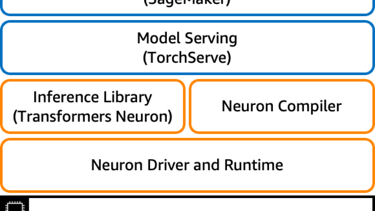
High performance Llama 2 deployments with AWS Inferentia2 using TorchServe

Recently, Llama 2 was released and has attracted a lot of interest from the machine learning community. Amazon EC2 Inf2 instances, powered by AWS Inferentia2, now support training and inference of Llama 2 models. In this post, we show low-latency and cost-effective inference of Llama-2 models on Amazon EC2 Inf2 instances using the latest AWS Neuron SDK release. We first introduce how to create, compile and deploy the Llama-2 model and explain the optimization techniques introduced by AWS Neuron SDK to achieve high performance at low cost. We then present our benchmarking results. Lastly, we show how the Llama-2 model can be deployed through Amazon SageMaker using TorchServe on an Inf2 instance.

What is Llama 2

Llama 2 is an auto-regressive language model that uses an optimized transformer architecture. Llama 2 is intended for commercial and research use in English. It comes in multiple sizes—7 billion, 13 billion, and 70 billion parameters—as well as pre-trained and fine-tuned variations. According to Meta, the tuned versions use supervised fine-tuning (SFT) and reinforcement learning with human feedback (RLHF) to align to human preferences for helpfulness and safety. Llama 2 was pre-trained on 2 trillion tokens of data from publicly available sources. The tuned models are intended for assistant-like chat, whereas pre-trained models can be adapted for a variety of natural language generation tasks. Regardless of which version of the model a developer uses, the responsible use guide from Meta can assist in guiding additional fine-tuning that may be necessary to customize and optimize the models with appropriate safety mitigations.

Amazon EC2 Inf2 instances Overview

Amazon EC2 Inf2 instances, featuring Inferentia2, provide 3x higher compute, 4x more accelerator memory, resulting in up to 4x higher throughput, and up to 10x lower latency, compared to the first generation Inf1 instances.

Large language model (LLM) inference is a memory bound workload, performance scales up with more accelerator memory bandwidth. Inf2 instances are the only inference optimized instances in Amazon EC2 to provide high speed accelerator interconnect (NeuronLink) enabling high performance large LLM model deployments with cost effective distributed inference. You can now efficiently and cost-effectively deploy billion-scale LLMs across multiple accelerators on Inf2 instances.

Inferentia2 supports FP32, TF32, BF16, FP16, UINT8, and the new configurable FP8 (cFP8) data type. AWS Neuron can take high-precision FP32 and FP16 models and autocast them to lower-precision data types while optimizing accuracy and performance. Autocasting reduces time to market by removing the need for lower-precision retraining and enabling higher-performance inference with smaller data types.

To make it flexible and extendable to deploy constantly evolving deep learning models, Inf2 instances have hardware optimizations and software support for dynamic input shapes as well as custom operators written in C++ through the standard PyTorch custom operator programming interfaces.

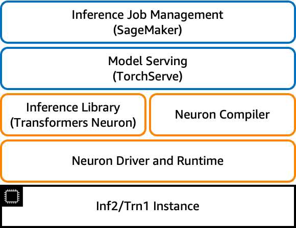
Transformers Neuron (transformers-neuronx)

Transformers Neuron is a software package that enables PyTorch users to deploy performance optimized LLM inference. It has an optimized version of transformer models implemented with XLA high level operators (HLO), which enables sharding tensors across multiple NeuronCores, a.k.a. tensor parallelism, and performance optimizations such as parallel context encoding and KV caching for Neuron hardware. The Llama 2 source code in XLA HLOs can be found here.

Llama 2 is supported in Transformers Neuron through the LlamaForSampling class. Transformers Neuron provides a seamless user experience with Hugging Face models to provide optimized inference on Inf2 instances. More details can be found from the Transforms Neuron Developer Guide. In the following section, we will explain how to deploy the Llama-2 13B model using Transformers Neuron. And, this example also applies to other Llama-based models.

Llama 2 model inference with Transformers Neuron

Create model, compile and deploy

We have three simple steps here to create, compile and deploy the model on Inf2 instances.

Create a CPU model, use this script or the following code snippet to serialize and save checkpoints in a local directory.

from transformers import AutoModelForCausalLM
from transformers_neuronx.module import save_pretrained_split
model_cpu = AutoModelForCausalLM.from_pretrained("meta-llama/Llama-2-13b-hf", low_cpu_mem_usage=True)
model_dir = "./llama-2-13b-split"
save_pretrained_split(model_cpu, model_dir)

Load and compile model from the local directory that you saved serialized checkpoints using the following.
To load the Llama 2 model, we use LlamaForSampling from Transformers Neuron. Note that the environment variable NEURON_RT_NUM_CORES specifies the number of NeuronCores to be used at runtime and it should match the tensor parallelism (TP) degree specified for the model. Also, NEURON_CC_FLAGS enables compiler optimization on decoder-only LLM models.

from transformers_neuronx.llama.model import LlamaForSampling
os.environ['NEURON_RT_NUM_CORES'] = '24'
os.environ['NEURON_CC_FLAGS'] = '--model-type=transformer'
model = LlamaForSampling.from_pretrained(
        model_dir,
        batch_size=1,
        tp_degree=24,
        amp='bf16',
        n_positions=16,
        context_length_estimate=[8]
    )

Now let’s compile the model and load model weights into device memory with a one liner API.

model.to_neuron()

Finally let’s run the inference on the compiled model. Note that both input and output of the sample function are a sequence of tokens.

inputs = torch.tensor([[1, 16644, 31844, 312, 31876, 31836, 260, 3067, 2228, 31844]])
seq_len = 16
outputs = model.sample(inputs, seq_len, top_k=1)

Inference optimizations in Transformers Neuron

Tensor parallelism

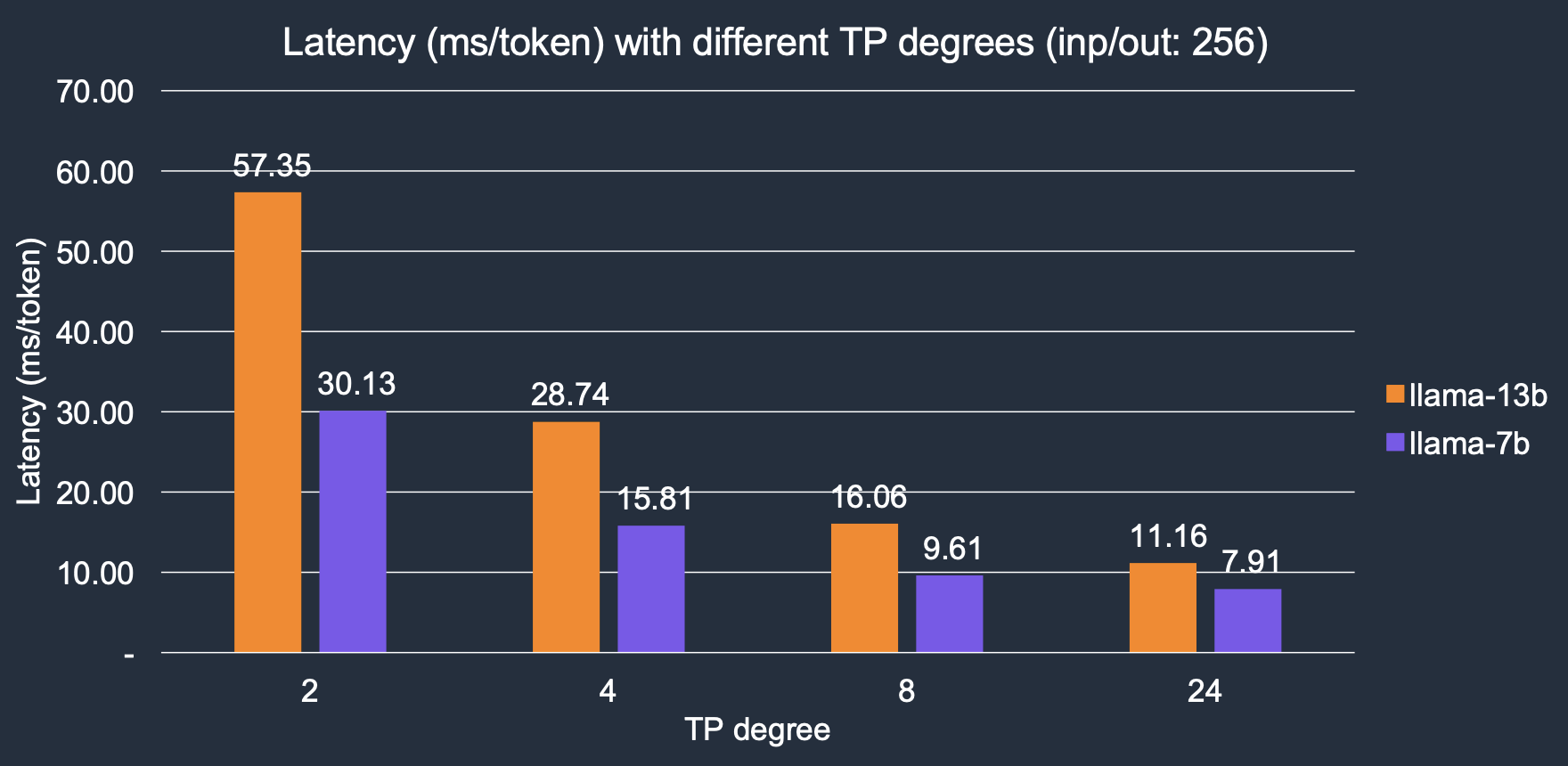
Transformer Neuron implements parallel tensor operations across multiple NeuronCores. We denote the number of cores to be used for inference as TP degree. Larger TP degree provides higher memory bandwidth, leading to lower latency, as LLM token generation is a memory-IO bound workload. With increasing the TP degree, the inference latency has decreased significantly, our results shows, ~4x overall speed up with increased TP degrees from 2 to 24. For the Llama-2 7B model, latency decreases from 30.1 ms/token with 2 cores to 7.9 ms/token with 24 cores; similarly for the Llama-2 13B model, it goes down from 57.3 ms/token to 11.1 ms/token.

Parallel context encoding

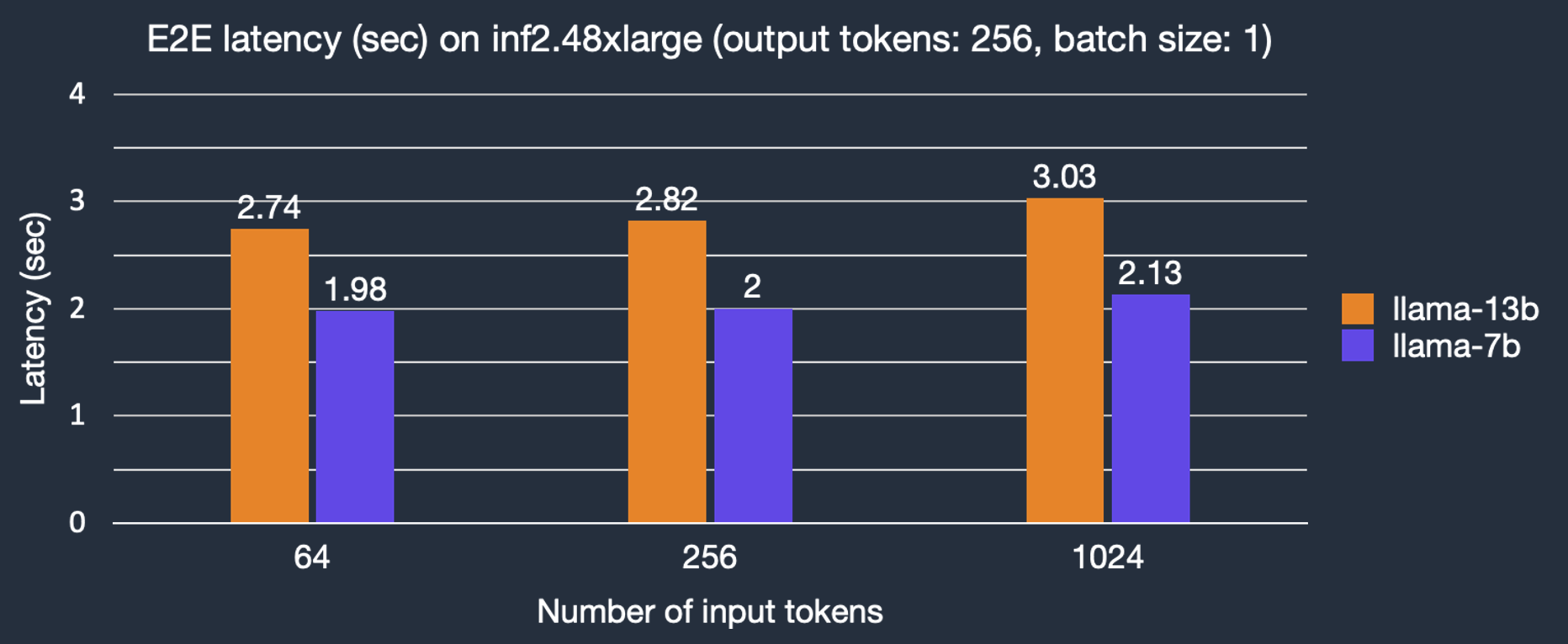
In the transformer architecture, tokens are produced in a sequential procedure called autoregressive sampling while input prompt tokens can be processed in parallel with parallel context encoding. This can significantly reduce the latency for input prompt context encoding before token generation through autoregressive sampling. By default, the parameter context_length_estimate would be set as a list of power-of-2 numbers which aims to cover a wide variety of context lengths. Depending on the use case, it can be set to custom numbers. This can be done when creating the Llama 2 model using LlamaForSampling.from_pretrained. We characterize the impact of input token length on end-to-end (E2E) latency. As shown in the figure, latency for text generation with the Llama-2 7B model only slightly increases with bigger input prompts, thanks to parallel context encoding.

KV caching

Self-attention block performs the self-attention operation with KV vectors. And, KV vectors are calculated using token embeddings and weights of KV and thus associated with tokens. In naive implementations, for each generated token, the entire KV cache is recalculated, but this reduces performance. Therefore Transformers Neuron library is reusing previously calculated KV vectors to avoid unnecessary computation, also known as KV caching, to reduce latency in the autoregressive sampling phase.

Benchmarking results

We benchmarked the latency and cost for both Llama-2 7B and 13B models under different conditions, i.e., number of output tokens, instance types. Unless specified, we use data type ‘bf16’ and batch size of 1 as this is a common configuration for real-time applications like chatbot and code assistant.

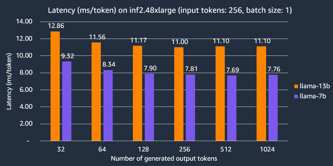
Latency

The following graphs shows the per token latency on inf2.48xlarge instance with TP degree 24. Here, the latency per output token is calculated as the end-to-end latency divided by the number of output tokens. Our experiments show Llama-2 7B end-to-end latency to generate 256 tokens is 2x faster compared to other comparable inference-optimized EC2 instances.

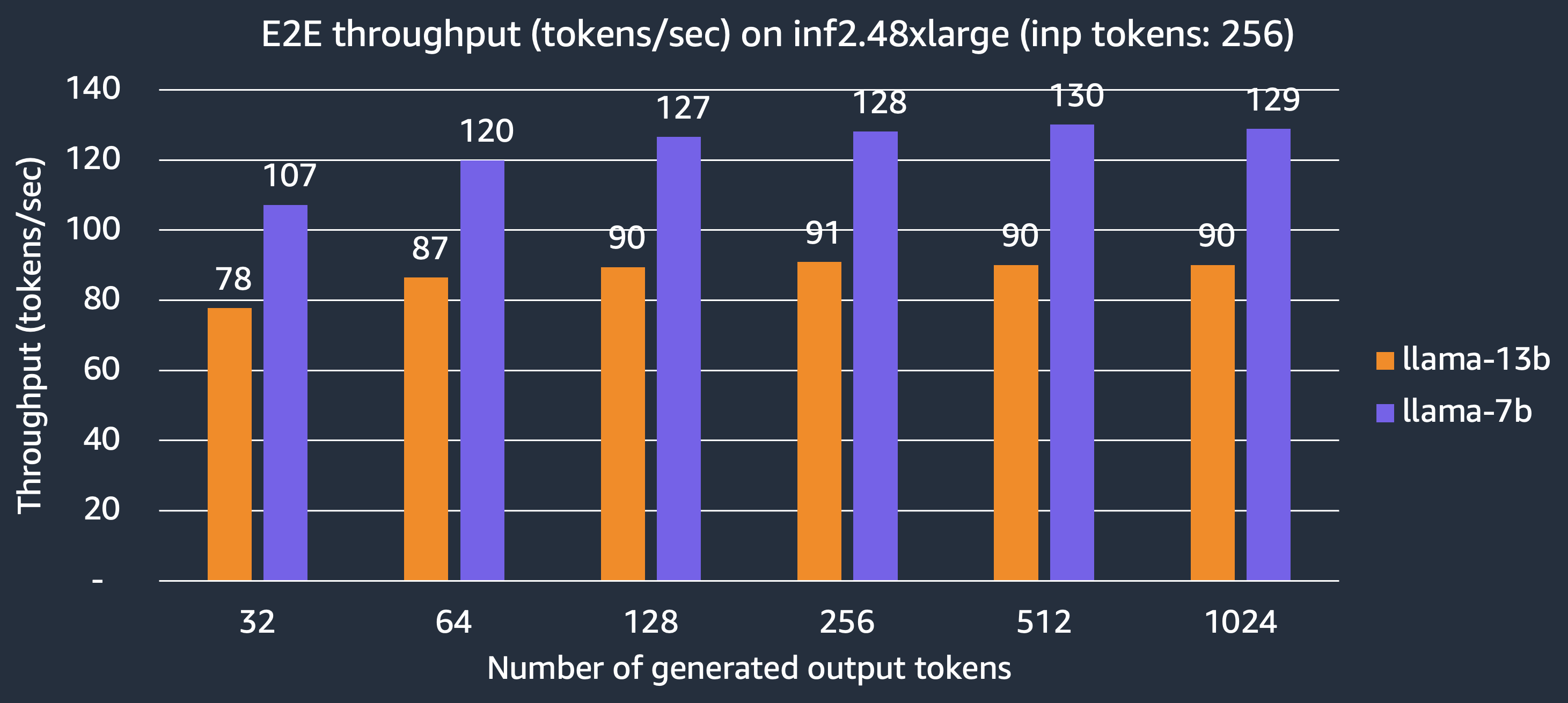
Throughput

We now show the number of tokens generated per second for the Llama-2 7B and 13B models that can be delivered by the inf2.48xlarge instance. With TP degree 24, fully utilizing all the 24 NeuronCores, we can achieve 130 tokens/sec and 90 tokens/sec for the Llama-2 7B and 13B models, respectively.

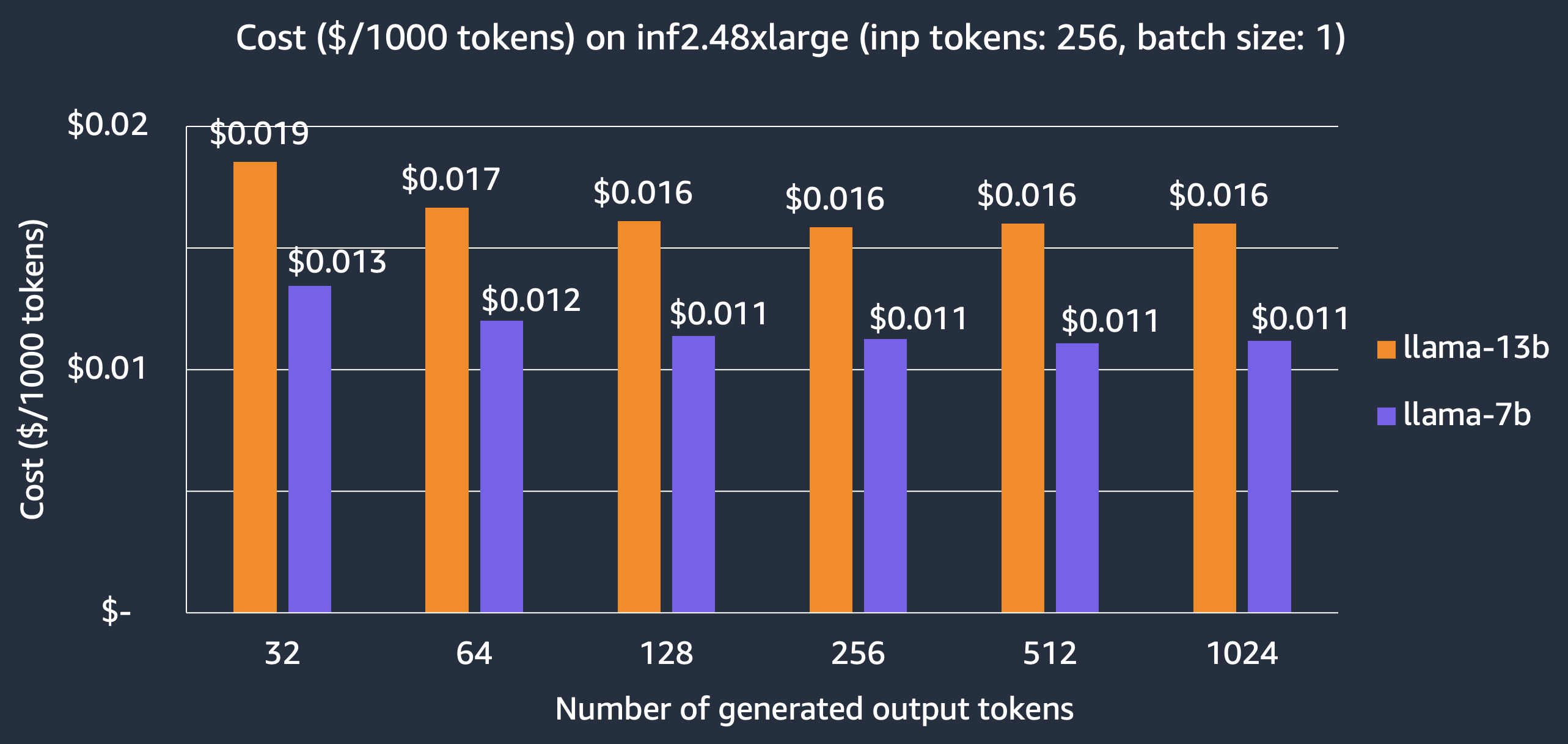
Cost

For latency-first applications, we show the cost of hosting Llama-2 models on the inf2.48xlarge instance, $0.011 per 1000 tokens and $0.016 per 1000 tokens for the 7B and 13B models, respectively, which achieve 3x cost saving over other comparable inference-optimized EC2 instances. Note that we report the cost based on 3-year reserved instance price which is what customers use for large production deployments.

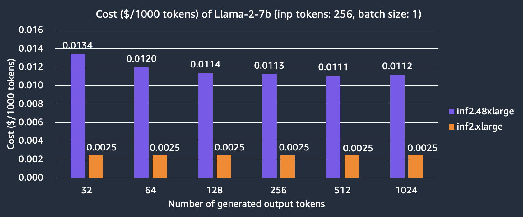
We also compare the cost of hosting the Llama-2 7B model on inf2.xlarge and inf2.48xlarge instances. We can see that inf2.xlarge is more than 4x cheaper than inf2.48xlarge but at the expense of longer latency due to smaller TP degree. For example, it takes 7.9 ms for the model to generate 256 output tokens with 256 input tokens on inf2.48xlarge but 30.1 ms on Inf2.xlarge.

Serving Llama2 with TorchServe on EC2 Inf2 instance

Now, we move on to model deployment. In this section, we show you how to deploy the Llama-2 13B model through SageMaker using TorchServe, which is the recommended model server for PyTorch, preinstalled in the AWS PyTorch Deep Learning Containers (DLC).

This section describes the preparation work needed for using TorchServe, particularly, how to configure model_config.yaml and inf2_handler.py as well as how to generate model artifacts and pre-compile the model for use in later model deployment. Preparing the model artifacts ahead-of-time avoids model compilation during model deployment and thus reduces the model loading time.

Model configuration model-config.yaml

The parameters defined in section handler and micro_batching are used in customer handler inf2_handler.py. More details about model_config.yaml are here. TorchServe micro-batching is a mechanism to pre-process and post-process a batch of inference requests in parallel. It is able to achieve higher throughput by better utilizing the available accelerator when the backend is steadily fed with incoming data, see here for more details. For model inference on Inf2, micro_batch_size, amp, tp_degree and max_length specify the batch size, data type, tensor parallelism degree and max sequence length, respectively.

# TorchServe Frontend Parameters
minWorkers: 1
maxWorkers: 1
maxBatchDelay: 100
responseTimeout: 10800
batchSize: 16

# TorchServe Backend Custom Handler Parameters
handler:
    model_checkpoint_dir: "llama-2-13b-split"
    amp: "bf16"
    tp_degree: 12
    max_length: 100

micro_batching:
    # Used by batch_size in function LlamaForSampling.from_pretrained
    micro_batch_size: 1  
    parallelism:
        preprocess: 2
        inference: 1
        postprocess: 2

Custom handler inf2_handler.py

Custom handler in Torchserve is a simple Python script that lets you define the model initialization, preprocessing, inference and post-processing logic as functions. Here, we create our Inf2 custom handler.

The initialize function is used to load the model. Here, Neuron SDK will compile the model for the first time and save the precompiled model in the directory as enabled by NEURONX_CACHE in the directory specified by NEURONX_DUMP_TO. After the first time, subsequent runs will check if there are already pre-compiled model artifacts. If so, it will skip model compilation.
Once the model is loaded, we initiate warm-up inference requests so that the compiled version is cached. When the neuron persistent cache is utilized, it can significantly reduce the model loading latency, ensuring that the subsequent inference runs swiftly.

os.environ["NEURONX_CACHE"] = "on"
os.environ["NEURONX_DUMP_TO"] = f"{model_dir}/neuron_cache"

TorchServe `TextIteratorStreamerBatch` extends Hugging Face transformers `BaseStreamer` to support response streaming when `batchSize` is larger than 1.

self.output_streamer = TextIteratorStreamerBatch(
    self.tokenizer,
    batch_size=self.handle.micro_batch_size,
    skip_special_tokens=True,
)

The inference function calls send_intermediate_predict_response to send the streaming response.

for new_text in self.output_streamer:
    logger.debug("send response stream")
    send_intermediate_predict_response(
        new_text[: len(micro_batch_req_id_map)],
        micro_batch_req_id_map,
        "Intermediate Prediction success",
        200,
        self.context,
    )

Package model artifacts

Package all the model artifacts into a folder llama-2-13b-neuronx-b1 using the torch-model-archiver.

torch-model-archiver --model-name llama-2-13b-neuronx-b1 --version 1.0 --handler inf2_handler.py -r requirements.txt --config-file model-config.yaml --archive-format no-archive

Serve the model

export TS_INSTALL_PY_DEP_PER_MODEL="true"
torchserve --ncs --start --model-store model_store --models llama-2-13b-neuronx-b1

Once the log shows “WORKER_MODEL_LOADED”, the pre-compiled model should be saved in the folder llama-2-13b-neuronx-b1/neuron_cache, which is tightly coupled with Neuron SDK version. Then, upload the folder llama-2-13b-neuronx-b1 to your S3 bucket for later use in the product deployment. The Llama-2 13B model artifacts in this blog can be found here, which is associated with Neuron SDK 2.13.2, in the TorchServe model zoo.

Deploy Llama-2 13B model on SageMaker Inf2 instance using TorchServe

In this section, we deploy the Llama-2 13B model using a PyTorch Neuronx container on a SageMaker endpoint with an ml.inf2.24xlarge hosting instance, which has 6 Inferentia2 accelerators corresponding to our model configuration model_config.yaml handler’s setting – tp_degree: 12. Given that we have packaged all the model artifacts into a folder using torch-model-archiver and uploaded to S3 bucket, we will now use the SageMaker Python SDK to create a SageMaker model and deploy it to a SageMaker real-time endpoint using the deploy uncompressed model method. Speed is the key benefit to deploying in this manner with SageMaker and you get a fully functional production ready endpoint complete with a secure RESTful endpoint without any effort spent on infrastructure. There are 3 steps to deploying the model and running inference on SageMaker. The notebook example can be found here.

Create a SageMaker model

from datetime import datetime

instance_type = "ml.inf2.24xlarge"
endpoint_name = sagemaker.utils.name_from_base("ts-inf2-llama2-13b-b1")

model = Model(
    name="torchserve-inf2-llama2-13b" + datetime.now().strftime("%Y-%m-%d-%H-%M-%S"),
    # Enable SageMaker uncompressed model artifacts
    model_data={
        "S3DataSource": {
                "S3Uri": s3_uri,
                "S3DataType": "S3Prefix",
                "CompressionType": "None",
        }
    },
    image_uri=container,
    role=role,
    sagemaker_session=sess,
    env={"TS_INSTALL_PY_DEP_PER_MODEL": "true"},
)

Deploy a SageMaker model

model.deploy(
    initial_instance_count=1,
    instance_type=instance_type,
    endpoint_name=endpoint_name,
    volume_size=512, # increase the size to store large model
    model_data_download_timeout=3600, # increase the timeout to download large model
    container_startup_health_check_timeout=600, # increase the timeout to load large model
)

Run streaming response inference on SageMaker
When the endpoint is in service, you can use the invoke_endpoint_with_response_stream API call to invoke the model. This feature enables the return of each generated token to the user, enhancing the user experience. It’s especially beneficial when generating an entire sequence is time-consuming.

import json

body = "Today the weather is really nice and I am planning on".encode('utf-8')
resp = smr.invoke_endpoint_with_response_stream(EndpointName=endpoint_name, Body=body, ContentType="application/json")
event_stream = resp['Body']
parser = Parser()
for event in event_stream:
    parser.write(event['PayloadPart']['Bytes'])
    for line in parser.scan_lines():
        print(line.decode("utf-8"), end=' ')

Sample inference:

Input

“Today the weather is really nice and I am planning on”

Output

“Today the weather is really nice and I am planning on going to the beach. I am going to take my camera and take some pictures of the beach. I am going to take pictures of the sand, the water, and the people. I am also going to take pictures of the sunset. I am really excited to go to the beach and take pictures.

The beach is a great place to take pictures. The sand, the water, and the people are all great subjects for pictures. The sunset is also a great subject for pictures.”

Conclusion

In this post, we showcased how to run Llama 2 model inference using Transformers Neuron and deploy Llama 2 model serving using TorchServe through Amazon SageMaker on an EC2 Inf2 instance. We demonstrated the benefits of using Inferentia2—low latency and low cost—enabled by optimizations in AWS Neuron SDK including tensor parallelism, parallel context encoding and KV caching, particularly for LLM inference. To stay up to date, please follow AWS Neuron’s latest release for new features.

Get started today with Llama 2 examples on EC2 and through SageMaker and stay tuned for how to optimize Llama 70B on Inf2!

Accelerate Foundation Models Research: Supporting a global academic research ecosystem for AI

The latest advances in artificial intelligence have sparked broad public interest and excitement, and the sciences are no exception. Increasingly capable foundation models are fuelling a fundamental shift in computing research, natural sciences, social sciences, and even computing education itself. As industry-led advances in AI continue to reach new heights, Microsoft Research believes that a vibrant and diverse research ecosystem is essential to realizing the promise of AI. This means ensuring that the academic research community, and especially researchers working outside computer science, can tap into these capabilities. Their depth and breadth of expertise across disciplines, cultures and languages can contribute meaningfully to our ability to use AI to address some of the world’s greatest technical, scientific, and societal challenges.

To this end, Microsoft Research has established Accelerate Foundation Models Research (AFMR), a new initiative that brings together an interdisciplinary research community to pursue three goals:

Aligning AI with shared human goals, values, and preferences via research on models, which enhances safety, robustness, sustainability, responsibility, and transparency, while also exploring new evaluation methods to measure the rapidly growing capabilities of new models.
Improving human interactions via sociotechnical research, which enables AI to extend human ingenuity, creativity and productivity, while also working to reduce inequities of access and working to ensure positive benefits for people and societies worldwide.
Accelerating scientific discovery in natural sciences through proactive knowledge discovery, hypothesis generation, and multiscale multimodal data generation.

AFMR is a global research network and a resource platform that enables researchers in computer science and many other disciplines to engage with some of the greatest technical and societal challenges of our time. This includes a grant program that provides access to state-of-the-art foundation models hosted through Microsoft Azure AI.

The goal is to foster more collaborations across disciplines, institutions, and sectors, and to unleash the full potential of AI for a wide range of research questions, applications, and societal contexts.

Following a successful pilot program and initial call for proposals (CFP), details of which are provided below, we are committed to continuing this work and can expect to solicit additional proposals throughout the coming year. Visit the AFMR site to learn more about upcoming programs and events, read peer-reviewed work that has resulted from the program and find resources to accelerate research and collaborations.

Inspiring research in the era of AI

When ChatGPT was released in the fall of 2022, it quickly became clear that this new technology and tool would play a central role in AI computing research and applications.

“As a natural language processing (NLP) researcher, I was excited at first by ChatGPT’s potential to stimulate an AI revolution,” said Evelyne Viegas, senior director of research engagement at Microsoft Research. “Soon, I became concerned about a potential lack of access to this resource outside of industry, which could delay important progress in academic settings.”

When Microsoft enabled access to OpenAI models (Embeddings series, GPT-3.5-Turbo series, and GPT-4 series) via the Azure AI services, it created an opportunity to engage with the academic community to learn about their needs and aspirations and start enabling them. A team at Microsoft Research conducted a pilot program offering model access to a small number of participants, and the success of this effort inspired a broader and more sustained program.

Research topics undertaken as part of the pilot reflect the ambitions of AI research at Microsoft in understanding general AI, driving model innovation, ensuring social benefit, transforming scientific discovery, and extending human capabilities across different domains (e.g., astronomy, education, health, law, society).

Although the research supported by this pilot is still underway, the examples below illustrate the possibilities of opening access to leading-edge models to a diverse group of researchers:

Integrating ChatGPT into English as a Foreign Language (EFL) Writing Education – Korea Advanced Institute of Science and Technology (KAIST)

This project explores how students can utilize generative AI for interactive revision in EFL writing. Because the majority of KAIST courses are given in English, the sooner non-English speakers can learn the language the better they will be able to participate in their classes. While earlier chatbots have been used for EFL, language learners found them unengaging. With Azure OpenAI Service, the KAIST team is gathering data to show how the unique capabilities of a GPT-4-based chatbot are accelerating learning while making the learner’s experience more engaging.

Lightweight Adaptation of LLMs for Healthcare Applications – Stanford University

This work focuses on accelerating the task of report summarization for radiologists to improve workflow and decrease the time needed to generate an accurate report. It uses domain adaptation via pretraining on biomedical text, or clinical text and discrete prompting or fine-tuning. Initial results are promising, showing the added value of using foundation models for some clinical tasks.

AI-Based Traffic Monitoring System using Physics-Informed Neural Networks and GPT Models – North Carolina A&T State University

Researchers are creating a traffic monitoring system using data collected from unmanned aerial vehicles (UAVs) to fine-tune foundation models for video analysis and traffic state estimation. This work can directly benefit transportation agencies and city planners, helping them understand traffic patterns, congestion, and safety hazards.

Forging New Horizons in Astronomy – Harvard University

This project seeks to enhance human interaction with astronomy literature utilizing the capabilities of the large language models (LLM), particularly GPT-4. This work employs in-context prompting techniques to expose the model to astronomy papers to build an astronomy-focused chat application to engage the broader community.

Expanding AFMR

Much experimentation remains to be done with foundation models. The AFMR CFP invited the community to develop proposals focused on the goals and questions below:

Aligning AI systems with human goals and preferences
Advancing beneficial applications of AI
Accelerating scientific discovery in the natural and life sciences

The response to the AFMR Fall CFP has been phenomenal, with close to 400 proposals from 170 universities across 33 countries.

“Research undertaken by the principal investigators brings the promise to advance research across a greater breadth of research pursuits, application domains, and societal contexts than we could have imagined,” Viegas said. “It covers a vast range of scientific and sociotechnical topics: creativity, culture, economy, education, finance, health, causality, evaluation, augmentation and adaptation, multimodal, responsible AI, robotics, scientific discovery, software and society. It is inspiring to see experts from different countries with different cultures, languages, institutions, and departments, including computer science, social science, natural sciences, humanities, medicine, music, all come together to work on democratizing AI and work on solving some of the greatest technical and societal challenges of tomorrow.”

The post Accelerate Foundation Models Research: Supporting a global academic research ecosystem for AI appeared first on Microsoft Research.

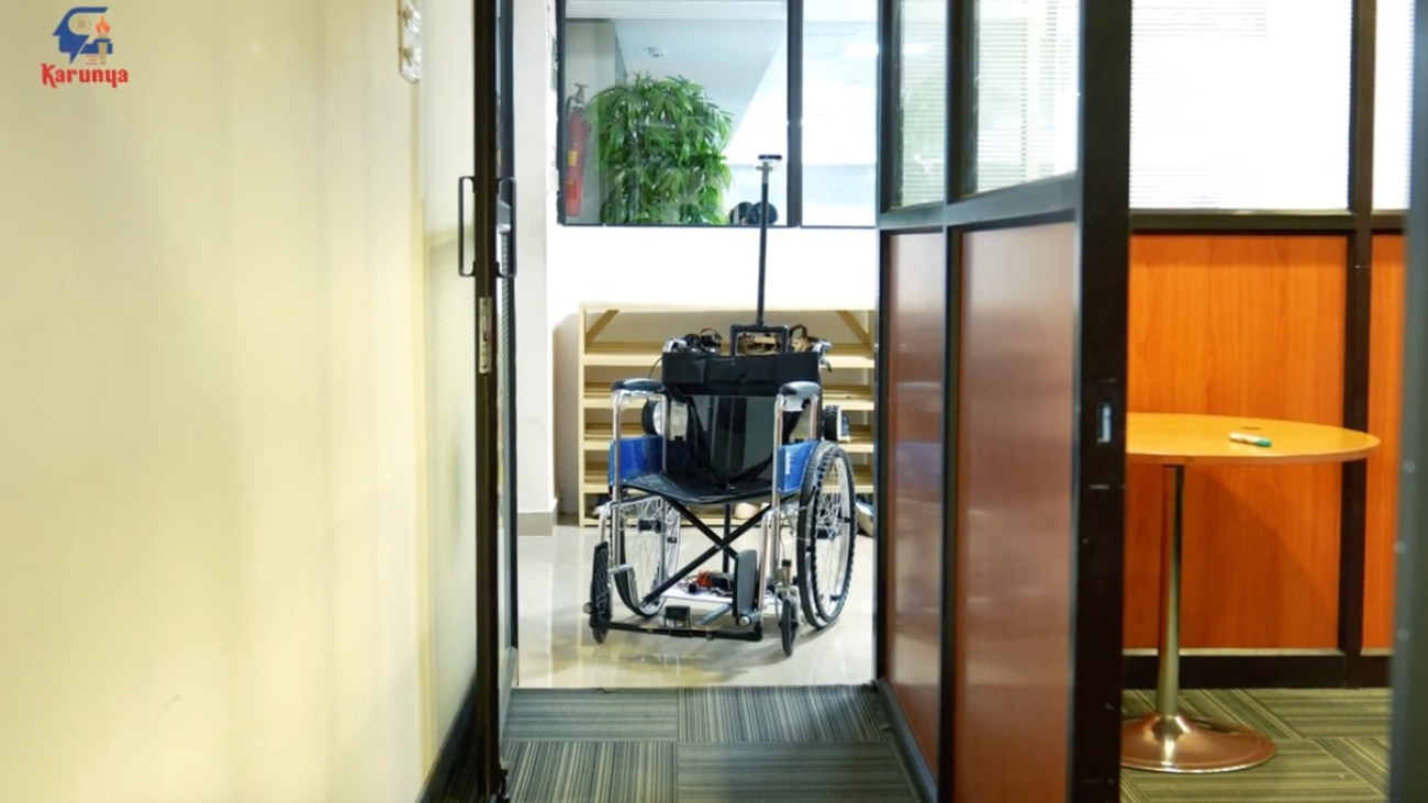
Meet the Maker: Robotics Student Rolls Out Autonomous Wheelchair With NVIDIA Jetson

With the help of AI, robots, tractors and baby strollers — even skate parks — are becoming autonomous. One developer, Kabilan KB, is bringing autonomous-navigation capabilities to wheelchairs, which could help improve mobility for people with disabilities.

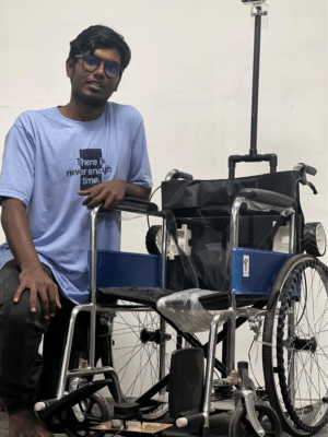
The undergraduate from the Karunya Institute of Technology and Sciences in Coimbatore, India, is powering his autonomous wheelchair project using the NVIDIA Jetson platform for edge AI and robotics.

The autonomous motorized wheelchair is connected to depth and lidar sensors — along with USB cameras — which allow it to perceive the environment and plan an obstacle-free path toward a user’s desired destination.

“A person using the motorized wheelchair could provide the location they need to move to, which would already be programmed in the autonomous navigation system or path-planned with assigned numerical values,” KB said. “For example, they could press ‘one’ for the kitchen or ‘two’ for the bedroom, and the autonomous wheelchair will take them there.”

An NVIDIA Jetson Nano Developer Kit processes data from the cameras and sensors in real time. It then uses deep learning-based computer vision models to detect obstacles in the environment.

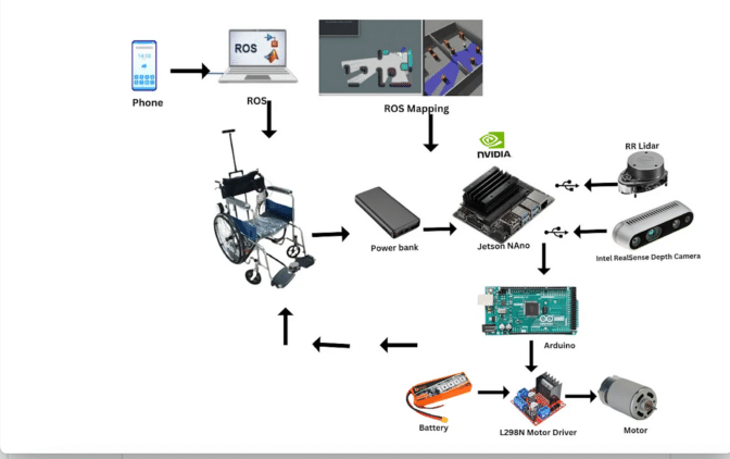
The developer kit acts as the brain of the autonomous system — generating a 2D map of its surroundings to plan a collision-free path to the destination — and sends updated signals to the motorized wheelchair to help ensure safe navigation along the way.

About the Maker

KB, who has a background in mechanical engineering, became fascinated with AI and robotics during the pandemic, when he spent his free time searching up educational YouTube videos on the topics.

He’s now working toward a bachelor’s degree in robotics and automation at the Karunya Institute of Technology and Sciences and aspires to one day launch a robotics startup.

KB, a self-described supporter of self-education, has also received several certifications from the NVIDIA Deep Learning Institute, including “Building Video AI Applications at the Edge on Jetson Nano” and “Develop, Customize and Publish in Omniverse With Extensions.”

Once he learned the basics of robotics, he began experimenting with simulation in NVIDIA Omniverse, a platform for building and operating 3D tools and applications based on the OpenUSD framework.

“Using Omniverse for simulation, I don’t need to invest heavily in prototyping models for my robots, because I can use synthetic data generation instead,” he said. “It’s the software of the future.”

His Inspiration

With this latest NVIDIA Jetson project, KB aimed to create a device that could be helpful for his cousin, who has a mobility disorder, and other people with disabilities who might not be able to control a manual or motorized wheelchair.

“Sometimes, people don’t have the money to buy an electric wheelchair,” KB said. “In India, only upper- and middle-class people can afford them, so I decided to use the most basic type of motorized wheelchair available and connect it to the Jetson to make it autonomous.”

The personal project was funded by the Program in Global Surgery and Social Change, which is jointly positioned under the Boston Children’s Hospital and Harvard Medical School.

His Jetson Project

After purchasing the basic motorized wheelchair, KB connected its motor hub with the NVIDIA Jetson Nano and lidar and depth cameras.

He trained the AI algorithms for the autonomous wheelchair using YOLO object detection on the Jetson Nano, as well as the Robot Operating System, or ROS, a popular software for building robotics applications.

The wheelchair can tap these algorithms to perceive and map its environment and plan a collision-free path.

“The NVIDIA Jetson Nano’s real-time processing speed prevents delays or lags for the user,” said KB, who’s been working on the project’s prototype since June. The developer dives into the technical components of the autonomous wheelchair on his blog. A demo of the autonomous wheelchair has also been featured on the Karunya Innovation and Design Studio YouTube channel.

Looking forward, he envisions his project could be expanded to allow users to control a wheelchair using brain signals from electroencephalograms, or EEGs, that are connected to machine learning algorithms.

“I want to make a product that would let a person with a full mobility disorder control their wheelchair by simply thinking, ‘I want to go there,’” KB said.

Learn more about the NVIDIA Jetson platform.

Scaling up learning across many different robot types

Robots are great specialists, but poor generalists. Typically, you have to train a model for each task, robot, and environment. Changing a single variable often requires starting from scratch. But what if we could combine the knowledge across robotics and create a way to train a general-purpose robot?Read More