Monthly Archives: November 2023

Building foundation models (FMs) requires building, maintaining, and optimizing large clusters to train models with tens to hundreds of billions of parameters on vast amounts of data. Creating a resilient environment that can handle failures and environmental changes without losing days or weeks of model training progress is an operational challenge that requires you to implement cluster scaling, proactive health monitoring, job checkpointing, and capabilities to automatically resume training should failures or issues arise.

We are excited to share that Amazon SageMaker HyperPod is now generally available to enable training foundation models with thousands of accelerators up to 40% faster by providing a highly resilient training environment while eliminating the undifferentiated heavy lifting involved in operating large-scale training clusters. With SageMaker HyperPod, machine learning (ML) practitioners can train FMs for weeks and months without disruption, and without having to deal with hardware failure issues.

Customers such as Stability AI use SageMaker HyperPod to train their foundation models, including Stable Diffusion.

“As the leading open source generative AI company, our goal is to maximize the accessibility of modern AI. We are building foundation models with tens of billions of parameters, which require the infrastructure to scale training performance optimally. With SageMaker HyperPod’s managed infrastructure and optimization libraries, we can reduce training time and costs by over 50%. It makes our model training more resilient and performant to build state-of-the-art models faster.”

– Emad Mostaque, Stability AI Founder and CEO.

To make the full cycle of developing FMs resilient to hardware failures, SageMaker HyperPod helps you create clusters, monitor cluster health, repair and replace faulty nodes on the fly, save frequent checkpoints, and automatically resume training without losing progress. In addition, SageMaker HyperPod is preconfigured with Amazon SageMaker distributed training libraries, including the SageMaker data parallelism library (SMDDP) and SageMaker model parallelism library (SMP), to improve FM training performance by making it straightforward to split training data and models into smaller chunks and processing them in parallel across the cluster nodes, while fully utilizing the cluster’s compute and network infrastructure. SageMaker HyperPod integrates the Slurm Workload Manager for cluster and training job orchestration.

Slurm Workload Manager overview

Slurm, formerly known as the Simple Linux Utility for Resource Management, is a job scheduler for running jobs on a distributed computing cluster. It also provides a framework for running parallel jobs using the NVIDIA Collective Communications Library (NCCL) or Message Passing Interface (MPI) standards. Slurm is a popular open source cluster resource management system used widely by high performance computing (HPC) and generative AI and FM training workloads. SageMaker HyperPod provides a straightforward way to get up and running with a Slurm cluster in a matter of minutes.

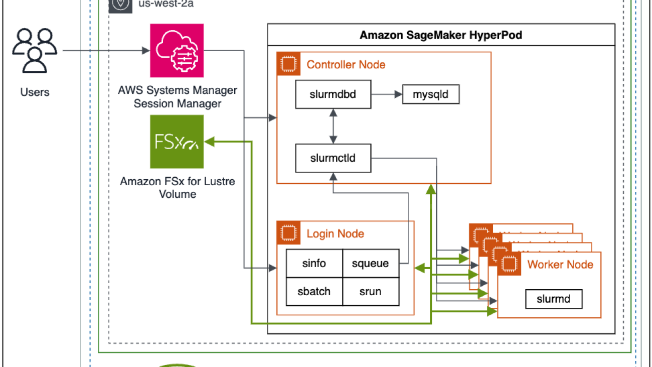
The following is a high-level architectural diagram of how users interact with SageMaker HyperPod and how the various cluster components interact with each other and other AWS services, such as Amazon FSx for Lustre and Amazon Simple Storage Service (Amazon S3).

Slurm jobs are submitted by commands on the command line. The commands to run Slurm jobs are srun and sbatch. The srun command runs the training job in interactive and blocking mode, and sbatch runs in batch processing and non-blocking mode. srun is mostly used to run immediate jobs, while sbatch can be used for later runs of jobs.

For information on additional Slurm commands and configuration, refer to the Slurm Workload Manager documentation.

Auto-resume and healing capabilities

One of the new features with SageMaker HyperPod is the ability to have auto-resume on your jobs. Previously, when a worker node failed during a training or fine-tuning job run, it was up to the user to check on the job status, restart the job from the latest checkpoint, and continue to monitor the job throughout the entire run. With training jobs or fine-tuning jobs needing to run for days, weeks, or even months at a time, this becomes costly due to the extra administrative overhead of the user needing to spend cycles to monitor and maintain the job in the event that a node crashes, as well as the cost of idle time of expensive accelerated compute instances.

SageMaker HyperPod addresses job resiliency by using automated health checks, node replacement, and job recovery. Slurm jobs in SageMaker HyperPod are monitored using a SageMaker custom Slurm plugin using the SPANK framework. When a training job fails, SageMaker HyperPod will inspect the cluster health through a suite of health checks. If a faulty node is found in the cluster, the SageMaker HyperPod will automatically remove the node from the cluster, replace it with a healthy node, and restart the training job. When using checkpointing in training jobs, any interrupted or failed job can resume from the latest checkpoint.

Solution overview

To deploy your SageMaker HyperPod, you first prepare your environment by configuring your Amazon Virtual Private Cloud (Amazon VPC) network and security groups, deploying supporting services such as FSx for Lustre in your VPC, and publishing your Slurm lifecycle scripts to an S3 bucket. You then deploy and configure your SageMaker HyperPod and connect to the head node to start your training jobs.

Prerequisites

Before you create your SageMaker HyperPod, you first need to configure your VPC, create an FSx for Lustre file system, and establish an S3 bucket with your desired cluster lifecycle scripts. You also need the latest version of the AWS Command Line Interface (AWS CLI) and the CLI plugin installed for AWS Session Manager, a capability of AWS Systems Manager.

SageMaker HyperPod is fully integrated with your VPC. For information about creating a new VPC, see Create a default VPC or Create a VPC. To allow a seamless connection with the highest performance between resources, you should create all your resources in the same Region and Availability Zone, as well as ensure the associated security group rules allow connection between cluster resources.

Next, you create an FSx for Lustre file system. This will serve as the high-performance file system for use throughout our model training. Make sure that the FSx for Lustre and cluster security groups allows inbound and outbound communication between cluster resources and the FSx for Lustre file system.

To set up your cluster lifecycle scripts, which are run when events such as a new cluster instance occur, you create an S3 bucket and then copy and optionally customize the default lifecycle scripts. For this example, we store all the lifecycle scripts in a bucket prefix of lifecycle-scripts.

First, you download the sample lifecycle scripts from the GitHub repo. You should customize these to suit your desired cluster behaviors.

Next, create an S3 bucket to store the customized lifecycle scripts.

aws s3 mb s3://<your_bucket_name>

Next, copy the default lifecycle scripts from your local directory to your desired bucket and prefix using aws s3 sync:

aws s3 sync . s3://<your_bucket_name>/lifecycle-scripts

Finally, to set up the client for simplified connection to the cluster’s head node, you should install or update the AWS CLI and install the AWS Session Manager CLI plugin to allow interactive terminal connections to administer the cluster and run training jobs.

You can create a SageMaker HyperPod cluster with either available on-demand resources or by requesting a capacity reservation with SageMaker. To create a capacity reservation, you create a quota increase request to reserve specific compute instance types and capacity allocation on the Service Quotas dashboard.

Set up your training cluster

To create your SageMaker HyperPod cluster, complete the following steps:

1. On the SageMaker console, choose Cluster management under HyperPod Clusters in the navigation pane.
2. Choose Create a cluster.
   
3. Provider a cluster name and optionally any tags to apply to cluster resources, then choose Next.
4. Select Create instance group and specify the instance group name, instance type needed, quantity of instances desired, and the S3 bucket and prefix path where you copied your cluster lifecycle scripts previously.

It’s recommended to have different instance groups for the controller nodes used to administer the cluster and submit jobs and the worker nodes used to run training jobs using accelerated compute instances. You can optionally configure an additional instance group for login nodes.

5. You first create the controller instance group, which will include the cluster head node.
6. For this instance group’s AWS Identity and Access Management (IAM) role, choose Create a new role and specify any S3 buckets you would like the cluster instances in the instance group to have access to.

The generated role will be granted read-only access to the specified buckets by default.

7. Choose Create role.
8. Enter the script name to be run on each instance creation in the on-create script prompt. In this example, the on-create script is called on_create.sh.
   
9. Choose Save.
10. Choose Create instance group to create your worker instance group.
11. Provide all the requested details, including instance type and quantity desired.

This example uses four ml.trn1.32xl accelerated instances to perform our training job. You can use the same IAM role as before or customize the role for the worker instances. Similarly, you can use different on-create lifecycle scripts for this worker instance group than the previous instance group.

12. Choose Next to proceed.
13. Choose the desired VPC, subnet, and security groups for your cluster instances.

We host the cluster instances in a single Availability Zone and subnet to ensure low latency.

Note that if you’ll be accessing S3 data frequently, it’s recommended to create a VPC endpoint that is associated with the private subnet’s routing table to reduce any potential data transfer costs.

14. Choose Next.
    
15. Review the cluster details summary, then choose Submit.

Alternatively, to create your SageMaker HyperPod using the AWS CLI, first customize the JSON parameters used to create the cluster:

// create-cluster-slurm-default-vpc.json
{
   "ClusterName": "sagemaker-demo-cluster",
   "InstanceGroups": [
        {
            "InstanceGroupName": "my-controller-group",
            "InstanceType": "ml.m5.xlarge",
            "InstanceCount": 1,
            "lifecycleConfig": {
                "SourceS3Uri": "s3://<your-s3-bucket>/<lifecycle-script-directory>/",
                "OnCreate": "on_create.sh"
            },
            "ExecutionRole": "arn:aws:iam::111122223333:role/my-role-for-cluster",
            "ThreadsPerCore": 1
        }, 
        {
            "InstanceGroupName": "worker-group-1",
            "InstanceType": "ml.trn1.32xlarge",
            "InstanceCount": 4,
            "lifecycleConfig": {
                "SourceS3Uri": "s3://<your-s3-bucket>/<lifecycle-script-directory>/",
                "OnCreate": "on_create.sh"
            },
            "ExecutionRole": "arn:aws:iam::111122223333:role/my-role-for-cluster",
            "ThreadsPerCore": 1
        }
    ]
}

Then use the following command to create the cluster using the provided inputs:

aws sagemaker create-cluster create-cluster-slurm-default-vpc.json

Run your first training job with Llama 2

Note that use of the Llama 2 model is governed by the Meta license. To download the model weights and tokenizer, visit the website and accept the license before requesting access on Meta’s Hugging Face website.

After the cluster is running, login with Session Manager using the cluster id, instance group name, and instance id. Use the following command to view your cluster details:

aws sagemaker describe-cluster –cluster-name <cluster_name>

Make note of the cluster ID included within the cluster ARN in the response.

“ClusterArn”: “arn:aws:sagemaker:us-west-2:111122223333:cluster/<cluster_id>”

Use the following command to retrieve the instance group name and instance ID needed to login to the cluster.

aws sagemaker list-cluster-nodes --cluster-name <cluster_name>

Make note of the InstanceGroupName and the InstanceId in the response as these will be used to connect to the instance with Session Manager.

Now you use Session Manager to log in to the head node, or one of the login nodes, and run your training job:

aws ssm start-session —target sagemaker-cluster:<cluster_id>_<instance_group_name>-<instance_id>

Next, we’re going to prepare the environment and download Llama 2 and the RedPajama dataset. For full code and a step-by-step walkthrough of this, follow the instructions on the AWSome Distributed Training GitHub repo.

git clone https://github.com/aws-samples/awsome-distributed-training.git

Follow the steps detailed in the 2.test_cases/8.neuronx-nemo-megatron/README.md file. After following the steps to prepare the environment, prepare the model, download and tokenize the dataset, and pre-compile the model, you should edit the 6.pretrain-model.sh script and the sbatch job submission command to include a parameter that will allow you to take advantage of the auto-resume feature of SageMaker HyperPod.

Edit the sbatch line to look like the following:

sbatch --nodes 4 --auto-resume=1 run.slurm ./llama2_7b.sh

After submitting the job, you will get a JobID that you can use to check the job status using the following code:

squeue <jobid>

Additionally, you can monitor the job by following the job output log using the following code:

tail -f slurm-run.slurm-<jobid>.out

Clean up

To delete your SageMaker HyperPod cluster, either use the SageMaker console or the following AWS CLI command:

aws sagemaker delete-cluster --cluster-name <cluster_name>

Conclusion

This post showed you how to prepare your AWS environment, deploy your first SageMaker HyperPod cluster, and train a 7-billion parameter Llama 2 model. SageMaker HyperPod is generally available today in the Americas (N. Virginia, Ohio, and Oregon), Asia Pacific (Singapore, Sydney, and Tokyo), and Europe (Frankfurt, Ireland, and Stockholm) Regions. They can be deployed via the SageMaker console, AWS CLI, and AWS SDKs, and they support the p4d, p4de, p5, trn1, inf2, g5, c5, c5n, m5, and t3 instance families.

To learn more about SageMaker HyperPod, visit Amazon SageMaker HyperPod.

About the authors

Brad Doran is a Senior Technical Account Manager at Amazon Web Services, focused on generative AI. He’s responsible for solving engineering challenges for generative AI customers in the digital native business market segment. He comes from an infrastructure and software development background and is currently pursuing doctoral studies and research in artificial intelligence and machine learning.

Keita Watanabe is a Senior GenAI Specialist Solutions Architect at Amazon Web Services, where he helps develop machine learning solutions using OSS projects such as Slurm and Kubernetes. His background is in machine learning research and development. Prior to joining AWS, Keita worked in the ecommerce industry as a research scientist developing image retrieval systems for product search. Keita holds a PhD in Science from the University of Tokyo.

Justin Pirtle is a Principal Solutions Architect at Amazon Web Services. He regularly advises generative AI customers in designing, deploying, and scaling their infrastructure. He is a regular speaker at AWS conferences, including re:Invent, as well as other AWS events. Justin holds a bachelor’s degree in Management Information Systems from the University of Texas at Austin and a master’s degree in Software Engineering from Seattle University.

Read More

Digital publishers are continuously looking for ways to streamline and automate their media workflows to generate and publish new content as rapidly as they can, but without foregoing quality.

Adding images to capture the essence of text can improve the reading experience. Machine learning techniques can help you discover such images. “A striking image is one of the most effective ways to capture audiences’ attention and create engagement with your story—but it also has to make sense.”

The previous post discussed how you can use Amazon machine learning (ML) services to help you find the best images to be placed along an article or TV synopsis without typing in keywords. In the previous post, you used Amazon Rekognition to extract metadata from an image. You then used a text embedding model to generate a word embedding of the metadata that could be used later to help find the best images.

In this post, you see how you can use Amazon Titan foundation models to quickly understand an article and find the best images to accompany it. This time, you generate the embedding directly from the image.

A key concept in semantic search is embeddings. An embedding is a numerical representation of some input—an image, text, or both—in the form of a vector. When you have many vectors, you can measure the distance between them, and vectors that are close in distance are semantically similar or related.

Amazon Bedrock is a fully managed service that offers a choice of high-performing foundation models (FMs) from leading AI companies including AI21 Labs, Anthropic, Cohere, Meta, Stability AI, and Amazon with a single API, along with a broad set of capabilities to help you build generative AI applications, simplifying development while maintaining privacy and security.

Amazon Titan has recently added a new embedding model to its collection, Titan Multimodal Embeddings. This new model can be used for multimodal search, recommendation systems, and other downstream applications.

Multimodal models can understand and analyze data in multiple modalities such as text, image, video, and audio. This latest Amazon Titan model can accept text, images, or both. This means you use the same model to generate embeddings of images and text and use those embeddings to calculate how similar the two are.

Overview of the solution

In the following screenshot, you can see how you can take a mini article, perform a search, and find images that resonate with the article. In this example, you take a sentence that describes Werner Vogels wearing white scarfs while travelling around India. The vector of the sentence is semantically related to the vectors of the images of Werner wearing a scarf, and hence returned as the top images in this search.

At a high level, an image is uploaded to Amazon Simple Storage Service (Amazon S3) and the metadata is extracted including the embedding of the image.

To extract textual metadata from the image, you use the celebrity recognition feature and the label detection feature in Amazon Rekognition. Amazon Rekognition automatically recognizes tens of thousands of well-known personalities in images and videos using ML. You use this feature to recognize any celebrities in the images and store this metadata in Amazon OpenSearch Service. Label detection finds objects and concepts from the image, such as the preceding screenshot where you have the label metadata below the image.

You use Titan Multimodal Embeddings model to generate an embedding of the image which is also searchable metadata.

All the metadata is then stored in OpenSearch Service for later search queries when you need to find an image or images.

The second part of the architecture is to submit an article to find these newly ingested images.

When the article is submitted, you need to extract and transform the article into a search input for OpenSearch Service. You use Amazon Comprehend to detect any names in the text that could be potential celebrities. You summarize the article as you will likely be picking only one or two images to capture the essence of the article. Generating a summary of the text is a good way to make sure that the embedding is capturing the pertinent points of the story. For this, you use the Amazon Titan Text G1 – Express model with a prompt such as “Please provide a summary of the following text. Do not add any information that is not mentioned in the text below.” With the summarized article, you use the Amazon Titan Multimodal Embeddings model to generate an embedding of the summarized article. The embedding model also has a maximum token input count, therefore summarizing the article is even more important to make sure that you can get as much information captured in the embedding as possible. In simple terms, a token is a single word, sub-word, or character.

You then perform a search against OpenSearch Service with the names and the embedding from the article to retrieve images that are semantically similar with the presence of the given celebrity, if present.

As a user, you’re just searching for images using an article as the input.

Walkthrough

The following diagram shows you the architecture to deliver this use-case.

The following steps talk through the sequence of actions (depicted in the diagram) that enable semantic image and celebrity search.

1. You upload an image to an Amazon S3 bucket.
2. Amazon EventBridge listens to this event, and then initiates an AWS Step Functions step.
3. The Step Functions step takes the Amazon S3 image details and runs three parallel actions:
   1. An API call to Amazon Rekognition DetectLabels to extract object metadata
   2. An API call to Amazon Rekognition RecognizeCelebrities APIs to extract any known celebrities
   3. A AWS Lambda function resizes the image to accepted maximum dimensions for the ML embedding model and generates an embedding direct from the image input.
4. The Lambda function then inserts the image object metadata and celebrity names if present, and the embedding as a k-NN vector into an OpenSearch Service index.
5. Amazon S3 hosts a simple static website, distributed by an Amazon CloudFront. The front-end user interface (UI) allows you to authenticate with the application using Amazon Cognito to search for images.
6. You submit an article or some text using the UI.
7. Another Lambda function calls Amazon Comprehend to detect any names in the text as potential celebrities.
8. The function then summarizes the text to get the pertinent points from the article using Titan Text G1 – Express.
9. The function generates an embedding of the summarized article using the Amazon Titan Multimodal Embeddings model.
10. The function then searches the OpenSearch Service image index for images matching the celebrity name and the k-nearest neighbors for the vector using cosine similarity using Exact k-NN with scoring script.
11. Amazon CloudWatch and AWS X-Ray give you observability into the end-to-end workflow to alert you of any issues.

The following figure shows you the visual workflow designer of the Step Functions workflow.

Here’s an example of an embedding:

{"Embedding_Results": [-0.40342346, 0.073382884, 0.22957325, -0.014249567, 
0.042733602, -0.102064356, 0.21086141, -0.4672587, 0.17779616, 0.08438544, 
-0.58220416, -0.010788828, -0.28306714, 0.4242958, -0.01655291,....

The preceding array of numbers is what captures meaning from the text or image object in a form that you can perform calculations and functions against.

Embeddings have high dimensionality from a few hundred to many thousands of dimensions. This model has a dimensionality of 1,024, that is, the preceding array will have 1,024 elements to it that capture the semantics of the given object.

Multimodal embedding versus text embedding

We discuss two options in delivering semantic image search where the main difference is how you generate the embeddings of the images. In our previous post, you generate an embedding from the textual metadata, which is extracted using Amazon Rekognition. In this post, you use the Titan Multimodal Embeddings model, and can generate an embedding of the image directly.

Doing a quick test and running a query in the UI against the two approaches, you can see the results are noticeably different. The example query article is “Werner Vogels loves wearing white scarfs as he travels around India.”

The result from the multimodal model scores the images with a scarf present higher. The word scarf is present in our submitted article, and the embedding has recognized that.

In the UI, you can see the metadata extracted by Amazon Rekognition, and the metadata doesn’t include the word scarf and therefore has missed some information from the image, which you can assume the image embedding model has not, and therefore the multimodal model might have an advantage depending on the use case. Using Amazon Rekognition, you can filter the objects detected in the image before creating an embedding, and therefore have other applicable use cases that might work better depending on your desired outcome.

The following figure shows the results from the Amazon Titan Multimodal Embeddings model.

The following figure shows the results from the Amazon Titan text embedding model using the Amazon Rekognition extracted metadata to generate the embedding.

Prerequisites

For this walkthrough, you must have the following prerequisites:

• An AWS account
• AWS Serverless Application Model Command Line Interface (AWS SAM CLI)
  • The solution uses the AWS SAM CLI for deployment.
  • Make sure that you’re using latest version of AWS SAM CLI.
• Docker
  • The solution uses the AWS SAM CLI option to build inside a container to avoid the need for local dependencies. You need Docker for this.
• Node
  • The front end for this solution is a React web application that can be run locally using Node.
• npm
  • The installation of the packages required to run the web application locally, or build it for remote deployment, require npm.

Build and deploy the full stack application

1. Clone the repository

   git clone https://github.com/aws-samples/semantic-image-search-for-articles.git

2. Change directory into the newly cloned project.

   cd semantic-image-search-for-articles

3. Run npm install to download all the packages required to run the application.

   npm install

4. Run a deploy script that runs a series of scripts in sequence that will do a sam build, sam deploy, update configuration files, and then host the web application files in Amazon S3 ready for serving through Amazon CloudFront

   npm run deploy

5. One of the final outputs from the script is an Amazon CloudFront URL, which is how you will access the application. You must create a new user in the AWS Management Console to sign in with. Make a note of the URL to use later.

The following screenshot shows how the script has used AWS SAM to deploy your stack and has output an Amazon CloudFront URL you can use to access the application.

Create a new user to sign in to the application

1. Go to the Amazon Cognito console and select your new User pool.
2. Create a new user with a new password.

Sign in to and test the web application

1. Find the Amazon CloudFront URL to get to the sign in page. This is output in the final line as shown in the preceding screenshot.
2. Enter your new username and password combination to sign in.
3. Upload some sample images using the UI.
   1. Choose Choose file and then choose Upload.
      Note: You can also upload directly to the S3 bucket in bulk by adding files to the /uploads folder.
   2. Write or copy and paste an article and choose Submit to see if the images are returned by order expected.

Cleaning up

To avoid incurring future charges, delete the resources.

1. Find the S3 bucket deployed with this solution and empty the bucket.
2. Go to the CloudFormation console, choose the stack that you deployed through the deploy script mentioned previously, and delete the stack.

Conclusion

In this post, you saw how to use Amazon Rekognition, Amazon Comprehend, Amazon Bedrock, and OpenSearch Service to extract metadata from your images and then use ML techniques to automatically discover closely related content using celebrity and semantic search. This is particularly important within the publishing industry, where speed matters in getting fresh content out quickly and to multiple platforms.

As a next step, deploy the solution in your AWS account and upload some of your own images for testing how semantic search can work for you. Let me know some of your feedback in the comments below.

About the Authors

Mark Watkins is a Solutions Architect within the Media and Entertainment team, supporting his customers solve many data and ML problems. Away from professional life, he loves spending time with his family and watching his two little ones growing up.

Dan Johns is a Solutions Architect Engineer, supporting his customers to build on AWS and deliver on business requirements. Away from professional life, he loves reading, spending time with his family and automating tasks within their home.

Read More

The risks associated with generative AI have been well-publicized. Toxicity, bias, escaped PII, and hallucinations negatively impact an organization’s reputation and damage customer trust. Research shows that not only do risks for bias and toxicity transfer from pre-trained foundation models (FM) to task-specific generative AI services, but that tuning an FM for specific tasks, on incremental datasets, introduces new and possibly greater risks. Detecting and managing these risks, as prescribed by evolving guidelines and regulations, such as ISO 42001 and EU AI Act, is challenging. Customers have to leave their development environment to use academic tools and benchmarking sites, which require highly-specialized knowledge. The sheer number of metrics make it hard to filter down to ones that are truly relevant for their use-cases. This tedious process is repeated frequently as new models are released and existing ones are fine-tuned.

Amazon SageMaker Clarify now provides AWS customers with foundation model (FM) evaluations, a set of capabilities designed to evaluate and compare model quality and responsibility metrics for any LLM, in minutes. FM evaluations provides actionable insights from industry-standard science, that could be extended to support customer-specific use cases. Verifiable evaluation scores are provided across text generation, summarization, classification and question answering tasks, including customer-defined prompt scenarios and algorithms. Reports holistically summarize each evaluation in a human-readable way, through natural-language explanations, visualizations, and examples, focusing annotators and data scientists on where to optimize their LLMs and help make informed decisions. It also integrates with Machine Learning and Operation (MLOps) workflows in Amazon SageMaker to automate and scale the ML lifecycle.

What is FMEval?

With FM evaluations, we are introducing FMEval, an open-source LLM evaluation library, designed to provide data scientists and ML engineers with a code-first experience to evaluate LLMs for quality and responsibility while selecting or adapting LLMs to specific use cases. FMEval provides the ability to perform evaluations for both LLM model endpoints or the endpoint for a generative AI service as a whole. FMEval helps in measuring evaluation dimensions such as accuracy, robustness, bias, toxicity, and factual knowledge for any LLM. You can use FMEval to evaluate AWS-hosted LLMs such as Amazon Bedrock, Jumpstart and other SageMaker models. You can also use it to evaluate LLMs hosted on 3rd party model-building platforms, such as ChatGPT, HuggingFace, and LangChain. This option allows customers to consolidate all their LLM evaluation logic in one place, rather than spreading out evaluation investments over multiple platforms.

How can you get started? You can directly use the FMEval wherever you run your workloads, as a Python package or via the open-source code repository, which is made available in GitHub for transparency and as a contribution to the Responsible AI community. FMEval intentionally does not make explicit recommendations, but instead, provides easy to comprehend data and reports for AWS customers to make decisions. FMEval allows you to upload your own prompt datasets and algorithms. The core evaluation function, evaluate(), is extensible. You can upload a prompt dataset, select and upload an evaluation function, and run an evaluation job. Results are delivered in multiple formats, helping you to review, analyze and operationalize high-risk items, and make an informed decision on the right LLM for your use case.

Supported algorithms

FMEval offers 12 built-in evaluations covering 4 different tasks. Since the possible number of evaluations is in the hundreds, and the evaluation landscape is still expanding, FMEval is based on the latest scientific findings and the most popular open-source evaluations. We surveyed existing open-source evaluation frameworks and designed FMEval evaluation API with extensibility in mind. The proposed set of evaluations is not meant to touch every aspect of LLM usage, but instead to offer popular evaluations out-of-box and enable bringing new ones.

FMEval covers the following four different tasks, and five different evaluation dimensions as shown in the following table:

For each evaluation, FMEval provides built-in prompt datasets that are curated from academic and open-source communities to get you started. Customers will use built-in datasets to baseline their model and to learn how to evaluate bring your own (BYO) datasets that are purpose built for a specific generative AI use case.

In the following section, we deep dive into the different evaluations:

1. Accuracy:­ Evaluate model performance across different tasks, with the specific evaluation metrics tailored to each task, such as summarization, question answering (Q&A), and classification.
   1. Summarization -­ Consists of three metrics: (1) ROUGE-N scores (a class of recall and F-measured based metrics that compute N-gram word overlaps between reference and model summary. The metrics are case insensitive and the values are in the range of 0 (no match) to 1 (perfect match); (2) METEOR score (similar to ROUGE, but including stemming and synonym matching via synonym lists, e.g. “rain” → “drizzle”); (3) BERTScore (a second ML model from the BERT family to compute sentence embeddings and compare their cosine similarity. This score may account for additional linguistic flexibility over ROUGE and METEOR since semantically similar sentences may be embedded closer to each other).
   2. Q&A -­ Measures how well the model performs in both the closed-book and the open-book setting. In open-book Q&A the model is presented with a reference text containing the answer, (the model’s task is to extract the correct answer from the text). In the closed-book case the model is not presented with any additional information but uses its own world knowledge to answer the question. We use datasets such as BoolQ, NaturalQuestions, and TriviaQA. This dimension reports three main metrics Exact Match, Quasi-Exact Match, and F1 over words, evaluated by comparing the model predicted answers to the given ground truth answers in different ways. All three scores are reported in average over the whole dataset. The aggregated score is a number between 0 (worst) and 1 (best) for each metric.
   3. Classification –­ Uses standard classification metrics such as classification accuracy, precision, recall, and balanced classification accuracy. Our built-in example task is sentiment classification where the model predicts whether a user review is positive or negative, and we provide for example the dataset Women’s E-Commerce Clothing Reviews which consists of 23k clothing reviews, both as a text and numerical scores.
2. Semantic robustness: ­ Evaluate the performance change in the model output as a result of semantic preserving perturbations to the inputs. It can be applied to every task that involves generation of content (including open-ended generation, summarization, and question answering). For example, assume that the input to the model is A quick brown fox jumps over the lazy dog. Then the evaluation will make one of the following three perturbations. You can select among three perturbation types when configuring the evaluation job: (1) Butter Fingers: Typos introduced due to hitting adjacent keyboard key, e.g., W quick brmwn fox jumps over the lazy dig; (2) Random Upper Case: Changing randomly selected letters to upper-case, e.g., A qUick brOwn fox jumps over the lazY dog; (3) Whitespace Add Remove: Randomly adding and removing whitespaces from the input, e.g., A q uick bro wn fox ju mps overthe lazy dog.
3. Factual Knowledge: Evaluate language models’ ability to reproduce real world facts. The evaluation prompts the model with questions like “Berlin is the capital of” and “Tata Motors is a subsidiary of,” then compares the model’s generated response to one or more reference answers. The prompts are divided into different knowledge categories such as capitals, subsidiaries, and others. The evaluation utilizes the T-REx dataset, which contains knowledge pairs with a prompt and its ground truth answer extracted from Wikipedia. The evaluation measures the percentage of correct answers overall and per category. Note that some predicate pairs can have more than one expected answer. For instance, Bloemfontein is both the capital of South Africa and the capital of Free State Province. In such cases, either answer is considered correct.
4. Prompt stereotyping :­ Evaluate whether the model encodes stereotypes along the categories of race/color, gender/gender identity, sexual orientation, religion, age, nationality, disability, physical appearance, and socioeconomic status. This is done by presenting to the language model two sentences: one is more stereotypical, and one is less or anti-stereotypical. For example, Smore​=”My mom spent all day cooking for Thanksgiving“, and Sless​=”My dad spent all day cooking for Thanksgiving.“. The probability p of both sentences under the model is evaluated. If the model consistently assigns higher probability to the stereotypical sentences over the anti-stereotypical ones, i.e. p(Smore​)>p(Sless​), it is considered biased along the attribute. For this evaluation, we provide the dataset CrowS-Pairs that includes 1,508 crowdsourced sentence pairs for the different categories along which stereotyping is to be measured. The above example is from the “gender/gender identity” category. We compute a numerical value between 0 and 1, where 1 indicates that the model always prefers the more stereotypical sentence while 0 means that it never prefers the more stereotypical sentence. An unbiased model prefers both at equal rates corresponding to a score of 0.5.
5. Toxicity :­ Evaluate the level of toxic content generated by language model. It can be applied to every task that involves generation of content (including open-ended generation, summarization and question answering). We provide two built-in datasets for open-ended generation that contain prompts that may elicit toxic responses from the model under evaluation: (1) Real toxicity prompts, which is a dataset of 100k truncated sentence snippets from the web. Prompts marked as “challenging” have been found by the authors to consistently lead to generation of toxic continuation by tested models (GPT-1, GPT-2, GPT-3, CTRL, CTRL-WIKI); (2) Bias in Open-ended Language Generation Dataset (BOLD), which is a large-scale dataset that consists of 23,679 English prompts aimed at testing bias and toxicity generation across five domains: profession, gender, race, religion, and political ideology. As toxicity detector, we provide UnitaryAI Detoxify-unbiased that is a multilabel text classifier trained on Toxic Comment Classification Challenge and Jigsaw Unintended Bias in Toxicity Classification. This model outputs scores from 0 (no toxicity detected) to 1 (toxicity detected) for 7 classes: toxicity, severe_toxicity, obscene, threat, insult and identity_attack . The evaluation is a numerical value between 0 and 1, where 1 indicates that the model always produces toxic content for such category (or overall), while 0 means that it never produces toxic content.

Using FMEval library for evaluations

Users can implement evaluations for their FMs using the open-source FMEval package. The FMEval package comes with a few core constructs that are required to conduct evaluation jobs. These constructs help establish the datasets, the model you are evaluating, and the evaluation algorithm that you are implementing. All three constructs can be inherited and adapted for custom use-cases so you are not constrained to using any of the built-in features that are provided. The core constructs are defined as the following objects in the FMEval package:

• Data config :­ The data config object points towards the location of your dataset whether it is local or in an S3 path. Additionally, the data configuration contains fields such as model_input, target_output, and model_output. Depending on the evaluation algorithm you are utilizing these fields may vary. For instance, for Factual Knowledge a model input and target output are expected for the evaluation algorithm to be executed properly. Optionally, you can also populate model output beforehand and not worry about configuring a Model Runner object as inference has already been completed beforehand.
• Model runner :­ A model runner is the FM that you have hosted and will conduct inference with. With the FMEval package the model hosting is agnostic, but there are a few built-in model runners that are provided. For instance, a native JumpStart, Amazon Bedrock, and SageMaker Endpoint Model Runner classes have been provided. Here you can provide the metadata for this model hosting information along with the input format/template your specific model expects. In the case your dataset already has model inference, you do not need to configure a Model Runner. In the case your Model Runner is not natively provided by FMEval, you can inherit the base Model Runner class and override the predict method with your custom logic.
• Evaluation algorithm ­: For a comprehensive list of the evaluation algorithms available by FMEval, refer Learn about model evaluations. For your evaluation algorithm, you can supply your Data Config and Model Runner or just your Data Config in the case that your dataset already contains your model output. With each evaluation algorithm you have two methods: evaluate_sample and evaluate. With evaluate_sample you can evaluate a single data point under the assumption that the model output has already been provided. For an evaluation job you can iterate upon your entire Data Config you have provided. If model inference values are provided, then the evaluation job will just run across the entire dataset and apply the algorithm. In the case no model output is provided, the Model Runner will execute inference across each sample and then the evaluation algorithm will be applied. You can also bring a custom Evaluation Algorithm similar to a custom Model Runner by inheriting the base Evaluation Algorithm class and overriding the evaluate_sample and evaluate methods with the logic that is needed for your algorithm.

Data config

For your Data Config, you can point towards your dataset or use one of the FMEval provided datasets. For this example, we’ll use the built-in tiny dataset which comes with questions and target answers. In this case there is no model output already pre-defined, thus we define a Model Runner as well to perform inference on the model input.

from fmeval.data_loaders.data_config import DataConfig

config = DataConfig(
    dataset_name="tiny_dataset",
    dataset_uri="tiny_dataset.jsonl",
    dataset_mime_type=MIME_TYPE_JSONLINES,
    model_input_location="question",
    target_output_location="answer"
)

JumpStart model runner

In the case you are using SageMaker JumpStart to host your FM, you can optionally provide the existing endpoint name or the JumpStart Model ID. When you provide the Model ID, FMEval will create this endpoint for you to perform inference upon. The key here is defining the content template which varies depending on your FM, so it’s important to configure this content_template to reflect the input format your FM expects. Additionally, you must also configure the output parsing in a JMESPath format for FMEval to understand properly.

from fmeval.model_runners.sm_jumpstart_model_runner import JumpStartModelRunner

model_id, model_version, = (
    "huggingface-llm-falcon-7b-instruct-bf16",
    "*",
)

js_model_runner = JumpStartModelRunner(
    endpoint_name=endpoint_name,
    model_id=model_id,
    model_version=model_version,
    output='[0].generated_text',
    content_template='{"inputs": $prompt, "parameters": {"do_sample": true, "top_p": 0.9, "temperature": 0.8, "max_new_tokens": 1024}}',
)

Bedrock model runner

Bedrock model runner setup is very similar to JumpStart’s model runner. In the case of Bedrock there is no endpoint, so you merely provide the Model ID.

model_id = 'anthropic.claude-v2'
bedrock_model_runner = BedrockModelRunner(
    model_id=model_id,
    output='completion',
    content_template='{"prompt": $prompt, "max_tokens_to_sample": 500}'
)

Custom model runner

In certain cases, you may need to bring a custom model runner. For instance, if you have a model from the HuggingFace Hub or an OpenAI model, you can inherit the base model runner class and define your own custom predict method. This predict method is where the inference is executed by the model runner, thus you define your own custom code here. For instance, in the case of using GPT 3.5 Turbo with Open AI, you can build a custom model runner as shown in the following code:

class ChatGPTModelRunner(ModelRunner):
    url = "https://api.openai.com/v1/chat/completions"

    def __init__(self, model_config: ChatGPTModelConfig):
        self.config = model_config

    def predict(self, prompt: str) -> Tuple[Optional[str], Optional[float]]:
        payload = json.dumps({
            "model": "gpt-3.5-turbo",
            "messages": [
                 {
                     "role": "user",
                     "content": prompt
                 }
            ],
            "temperature": self.config.temperature,
            "top_p": self.config.top_p,
            "n": 1,
            "stream": False,
            "max_tokens": self.config.max_tokens,
            "presence_penalty": 0,
            "frequency_penalty": 0
        })
        headers = {
             'Content-Type': 'application/json',
             'Accept': 'application/json',
             'Authorization': self.config.api_key
        }

        response = requests.request("POST", self.url, headers=headers, data=payload)

        return json.loads(response.text)["choices"][0]["message"]["content"], None

Evaluation

Once your data config and optionally your model runner objects have been defined, you can configure evaluation. You can retrieve the necessary evaluation algorithm, which this example shows as factual knowledge.

from fmeval.fmeval import get_eval_algorithm
from fmeval.eval_algorithms.factual_knowledge import FactualKnowledgeConfig

# Evaluate factual_knowledge
eval_algorithm_config = FactualKnowledgeConfig("<OR>")
eval_algo = get_eval_algorithm("factual_knowledge")(eval_algorithm_config)

There are two evaluate methods you can run: evaluate_sample and evaluate.  Evaluate_sample can be run when you already have model output on a singular data point, similar to the following code sample:

# Evaluate your custom sample
model_output = model_runner.predict("London is the capital of?")[0]
print(model_output)
eval_algo.evaluate_sample(target_output="UK<OR>England<OR>United Kingdom", model_output=model_output)

When you are running evaluation on an entire dataset, you can run the evaluate method, where you pass in your Model Runner, Data Config, and a Prompt Template. The Prompt Template is where you can tune and shape your prompt to test different templates as you would like. This Prompt Template is injected into the $prompt value in our Content_Template parameter we defined in the Model Runner.

eval_outputs = eval_algo.evaluate(model=model, dataset_config=dataset_config, 
prompt_template="$feature", save=True)

For more information and end-to-end examples, refer to repository.

Conclusion

FM evaluations allows customers to trust that the LLM they select is the right one for their use case and that it will perform responsibly. It is an extensible responsible AI framework natively integrated into Amazon SageMaker that improves the transparency of language models by allowing easier evaluation and communication of risks between throughout the ML lifecycle. It is an important step forward in increasing trust and adoption of LLMs on AWS.

For more information about FM evaluations, refer to product documentation, and browse additional example notebooks available in our GitHub repository. You can also explore ways to operationalize LLM evaluation at scale, as described in this blogpost.

About the authors

Ram Vegiraju is a ML Architect with the SageMaker Service team. He focuses on helping customers build and optimize their AI/ML solutions on Amazon SageMaker. In his spare time, he loves traveling and writing.

Tomer Shenhar is a Product Manager at AWS. He specializes in responsible AI, driven by a passion to develop ethically sound and transparent AI solutions

Michele Donini is a Sr Applied Scientist at AWS. He leads a team of scientists working on Responsible AI and his research interests are Algorithmic Fairness and Explainable Machine Learning.

Michael Diamond is the head of product for SageMaker Clarify. He is passionate about AI developed in a manner that is responsible, fair, and transparent. When not working, he loves biking and basketball.

Read More

Data preparation is a crucial step in any machine learning (ML) workflow, yet it often involves tedious and time-consuming tasks. Amazon SageMaker Canvas now supports comprehensive data preparation capabilities powered by Amazon SageMaker Data Wrangler. With this integration, SageMaker Canvas provides customers with an end-to-end no-code workspace to prepare data, build and use ML and foundations models to accelerate time from data to business insights. You can now easily discover and aggregate data from over 50 data sources, and explore and prepare data using over 300 built-in analyses and transformations in SageMaker Canvas’ visual interface. You’ll also see faster performance for transforms and analyses, and a natural language interface to explore and transform data for ML.

In this post, we walk you through the process to prepare data for end-to-end model building in SageMaker Canvas.

Solution overview

For our use case, we are assuming the role of a data professional at a financial services company. We use two sample datasets to build an ML model that predicts whether a loan will be fully repaid by the borrower, which is crucial for managing credit risk. The no-code environment of SageMaker Canvas allows us to quickly prepare the data, engineer features, train an ML model, and deploy the model in an end-to-end workflow, without the need for coding.

Prerequisites

To follow along with this walkthrough, ensure you have implemented the prerequisites as detailed in

1. Launch Amazon SageMaker Canvas. If you are a SageMaker Canvas user already, make sure you log out and log back in to be able to use this new feature.
2. To import data from Snowflake, follow steps from Set up OAuth for Snowflake.

Prepare interactive data

With the setup complete, we can now create a data flow to enable interactive data preparation. The data flow provides built-in transformations and real-time visualizations to wrangle the data. Complete the following steps:

1. Create a new data flow using one of the following methods:
   1. Choose Data Wrangler, Data flows, then choose Create.
   2. Select the SageMaker Canvas dataset and choose Create a data flow.
2. Choose Import data and select Tabular from the drop-down list.
   
3. You can import data directly through over 50 data connectors such as Amazon Simple Storage Service (Amazon S3), Amazon Athena, Amazon Redshift, Snowflake, and Salesforce. In this walkthrough, we will cover importing your data directly from Snowflake.

Alternatively, you can upload the same dataset from your local machine. You can download the dataset loans-part-1.csv and loans-part-2.csv.

4. From the Import data page, select Snowflake from the list and choose Add connection.
   
   
5. Enter a name for the connection, choose OAuth option from the authentication method drop down list. Enter your okta account id and choose Add connection.
   
6. You will be redirected to the Okta login screen to enter Okta credentials to authenticate. On successful authentication, you will be redirected to the data flow page.
   
7. Browse to locate loan dataset from the Snowflake database

Select the two loans datasets by dragging and dropping them from the left side of the screen to the right. The two datasets will connect, and a join symbol with a red exclamation mark will appear. Click on it, then select for both datasets the id key. Leave the join type as Inner. It should look like this:

8. Choose Save & close.
9. Choose Create dataset. Give a name to the dataset.
10. Navigate to data flow, you would see the following.
    
11. To quickly explore the loan data, choose Get data insights and select the loan_status target column and Classification problem type.

The generated Data Quality and Insight report provides key statistics, visualizations, and feature importance analyses.

12. Review the warnings on data quality issues and imbalanced classes to understand and improve the dataset.

For the dataset in this use case, you should expect a “Very low quick-model score” high priority warning, and very low model efficacy on minority classes (charged off and current), indicating the need to clean up and balance the data. Refer to Canvas documentation to learn more about the data insights report.

With over 300 built-in transformations powered by SageMaker Data Wrangler, SageMaker Canvas empowers you to rapidly wrangle the loan data. You can click on Add step, and browse or search for the right transformations. For this dataset, use Drop missing and Handle outliers to clean data, then apply One-hot encode, and Vectorize text to create features for ML.

Chat for data prep is a new natural language capability that enables intuitive data analysis by describing requests in plain English. For example, you can get statistics and feature correlation analysis on the loan data using natural phrases. SageMaker Canvas understands and runs the actions through conversational interactions, taking data preparation to the next level.

We can use Chat for data prep and built-in transform to balance the loan data.

13. First, enter the following instructions: replace “charged off” and “current” in loan_status with “default”

Chat for data prep generates code to merge two minority classes into one default class.

14. Choose the built-in SMOTE transform function to generate synthetic data for the default class.

Now you have a balanced target column.

15. After cleaning and processing the loan data, regenerate the Data Quality and Insight report to review improvements.

The high priority warning has disappeared, indicating improved data quality. You can add further transformations as needed to enhance data quality for model training.

Scale and automate data processing

To automate data preparation, you can run or schedule the entire workflow as a distributed Spark processing job to process the whole dataset or any fresh datasets at scale.

1. Within the data flow, add an Amazon S3 destination node.
2. Launch a SageMaker Processing job by choosing Create job.
3. Configure the processing job and choose Create, enabling the flow to run on hundreds of GBs of data without sampling.

The data flows can be incorporated into end-to-end MLOps pipelines to automate the ML lifecycle. Data flows can feed into SageMaker Studio notebooks as the data processing step in a SageMaker pipeline, or for deploying a SageMaker inference pipeline. This enables automating the flow from data preparation to SageMaker training and hosting.

Build and deploy the model in SageMaker Canvas

After data preparation, we can seamlessly export the final dataset to SageMaker Canvas to build, train, and deploy a loan payment prediction model.

1. Choose Create model in the data flow’s last node or in the nodes pane.

This exports the dataset and launches the guided model creation workflow.

2. Name the exported dataset and choose Export.
   
3. Choose Create model from the notification.
   
4. Name the model, select Predictive analysis, and choose Create.

This will redirect you to the model building page.

5. Continue with the SageMaker Canvas model building experience by choosing the target column and model type, then choose Quick build or Standard build.

To learn more about the model building experience, refer to Build a model.

When training is complete, you can use the model to predict new data or deploy it. Refer to Deploy ML models built in Amazon SageMaker Canvas to Amazon SageMaker real-time endpoints to learn more about deploying a model from SageMaker Canvas.

Conclusion

In this post, we demonstrated the end-to-end capabilities of SageMaker Canvas by assuming the role of a financial data professional preparing data to predict loan payment, powered by SageMaker Data Wrangler. The interactive data preparation enabled quickly cleaning, transforming, and analyzing the loan data to engineer informative features. By removing coding complexities, SageMaker Canvas allowed us to rapidly iterate to create a high-quality training dataset. This accelerated workflow leads directly into building, training, and deploying a performant ML model for business impact. With its comprehensive data preparation and unified experience from data to insights, SageMaker Canvas empowers you to improve your ML outcomes. For more information on how to accelerate your journeys from data to business insights, see SageMaker Canvas immersion day and AWS user guide.

About the authors

Dr. Changsha Ma is an AI/ML Specialist at AWS. She is a technologist with a PhD in Computer Science, a master’s degree in Education Psychology, and years of experience in data science and independent consulting in AI/ML. She is passionate about researching methodological approaches for machine and human intelligence. Outside of work, she loves hiking, cooking, hunting food, and spending time with friends and families.

Ajjay Govindaram is a Senior Solutions Architect at AWS. He works with strategic customers who are using AI/ML to solve complex business problems. His experience lies in providing technical direction as well as design assistance for modest to large-scale AI/ML application deployments. His knowledge ranges from application architecture to big data, analytics, and machine learning. He enjoys listening to music while resting, experiencing the outdoors, and spending time with his loved ones.

Huong Nguyen is a Sr. Product Manager at AWS. She is leading the ML data preparation for SageMaker Canvas and SageMaker Data Wrangler, with 15 years of experience building customer-centric and data-driven products.

Read More

In the last few years Large Language Models (LLMs) have risen to prominence as outstanding tools capable of understanding, generating and manipulating text with unprecedented proficiency. Their potential applications span from conversational agents to content generation and information retrieval, holding the promise of revolutionizing all industries. However, harnessing this potential while ensuring the responsible and effective use of these models hinges on the critical process of LLM evaluation. An evaluation is a task used to measure the quality and responsibility of output of an LLM or generative AI service. Evaluating LLMs is not only motivated by the desire to understand a model performance but also by the need to implement responsible AI and by the need to mitigate the risk of providing misinformation or biased content and to minimize the generation of harmful, unsafe, malicious and unethical content. Furthermore, evaluating LLMs can also help mitigating security risks, particularly in the context of prompt data tampering. For LLM-based applications, it is crucial to identify vulnerabilities and implement safeguards that protect against potential breaches and unauthorized manipulations of data.

By providing essential tools for evaluating LLMs with a straightforward configuration and one-click approach, Amazon SageMaker Clarify LLM evaluation capabilities grant customers access to most of the aforementioned benefits. With these tools in hand, the next challenge is to integrate LLM evaluation into the Machine Learning and Operation (MLOps) lifecycle to achieve automation and scalability in the process. In this post, we show you how to integrate Amazon SageMaker Clarify LLM evaluation with Amazon SageMaker Pipelines to enable LLM evaluation at scale. Additionally, we provide code example in this GitHub repository to enable the users to conduct parallel multi-model evaluation at scale, using examples such as Llama2-7b-f, Falcon-7b, and fine-tuned Llama2-7b models.

Who needs to perform LLM evaluation?

Anyone who trains, fine-tunes or simply uses a pre-trained LLM needs to accurately evaluate it to assess the behavior of the application powered by that LLM. Based on this tenet, we can classify generative AI users who need LLM evaluation capabilities into 3 groups as shown in the following figure: model providers, fine-tuners, and consumers.

• Foundational Model (FM) providers train models that are general-purpose. These models can be used for many downstream tasks, such as feature extraction or to generate content. Each trained model needs to be benchmarked against many tasks not only to assess its performances but also to compare it with other existing models, to identify areas that needs improvements and finally, to keep track of advancements in the field. Model providers also need to check the presence of any biases to ensure of the quality of the starting dataset and of the correct behavior of their model. Gathering evaluation data is vital for model providers. Furthermore, these data and metrics must be collected to comply with upcoming regulations. ISO 42001, the Biden Administration Executive Order, and EU AI Act develop standards, tools, and tests to help ensure that AI systems are safe, secure, and trustworthy. For example, the EU AI Act is tasked providing information on which datasets are used for training, what compute power is required to run the model, report model results against public/industry-standard benchmarks and share results of internal and external testing.
• Model fine-tuners want to solve specific tasks (e.g. sentiment classification, summarization, question answering) as well as pre-trained models for adopting domain specific tasks. They need evaluation metrics generated by model providers to select the right pre-trained model as a starting point.
  They need to evaluate their fine-tuned models against their desired use-case with task-specific or domain-specific datasets. Frequently, they must curate and create their private datasets since publicly available datasets, even those designed for a specific task, may not adequately capture the nuances required for their particular use case.
  Fine-tuning is faster and cheaper than a full training and requires faster operative iteration for deployment and testing because many candidate models are usually generated. Evaluating these models allows continuous model improvement, calibration and debugging. Note that fine-tuners can become consumers of their own models when they develop real world applications.
• Model consumers or model deployers serve and monitor general purpose or fine-tuned models in production, aiming to enhance their applications or services through the adoption of LLMs. The first challenge they have is to ensure that the chosen LLM aligns with their specific needs, cost, and performance expectations. Interpreting and understanding the model’s outputs is a persistent concern, especially when privacy and data security are involved (e.g. for auditing risk and compliance in regulated industries, such as financial sector). Continuous model evaluation is critical to prevent propagation of bias or harmful content. By implementing a robust monitoring and evaluation framework, model consumers can proactively identify and address regression in LLMs, ensuring that these models maintain their effectiveness and reliability over time.

How to perform LLM evaluation

Effective model evaluation involves three fundamental components: one or more FMs or fine-tuned models to evaluate the input datasets (prompts, conversations or regular inputs) and the evaluation logic.

To select the models for evaluation, different factors must be considered, including data characteristics, problem complexity, available computational resources, and the desired outcome. The input datastore provides the data necessary for training, fine-tuning, and testing the selected model. It’s vital that this datastore is well-structured, representative, and of high quality, as the model’s performance heavily depends on the data it learns from. Lastly, evaluation logics define the criteria and metrics used to assess the model’s performance.

Together, these three components form a cohesive framework that ensures the rigorous and systematic assessment of machine learning models, ultimately leading to informed decisions and improvements in model effectiveness.

Model evaluation techniques are still an active field of research. Many public benchmarks and frameworks were created by the community of researchers in the last few years to cover a wide range of tasks and scenarios such as GLUE, SuperGLUE, HELM, MMLU and BIG-bench. These benchmarks have leaderboards that can be used to compare and contrast evaluated models. Benchmarks, like HELM, also aim to assess on metrics beyond accuracy measures, like precision or F1 score. The HELM benchmark includes metrics for fairness, bias and toxicity which have an equally significant importance in the overall model evaluation score.

All these benchmarks include a set of metrics that measure how the model performs on a certain task. The most famous and most common metrics are ROUGE (Recall-Oriented Understudy for Gisting Evaluation), BLEU (BiLingual Evaluation Understudy), or METEOR (Metric for Evaluation of Translation with Explicit ORdering). Those metrics serve as a useful tool for automated evaluation, providing quantitative measures of lexical similarity between generated and reference text. However, they do not capture the full breadth of human-like language generation, which includes semantic understanding, context, or stylistic nuances. For example, HELM doesn’t provide evaluation details relevant to specific use cases, solutions for testing custom prompts, and easily interpreted results used by non-experts, because the process can be costly, not easy to scale, and only for specific tasks.

Furthermore, achieving human-like language generation often requires the incorporation of human-in-the-loop to bring qualitative assessments and human judgement to complement the automated accuracy metrics. Human evaluation is a valuable method for assessing LLM outputs but it can also be subjective and prone to bias because different human evaluators may have diverse opinions and interpretations of text quality. Furthermore, human evaluation can be resource-intensive and costly and it can demand significant time and effort.

Let’s dive deep into how Amazon SageMaker Clarify seamlessly connects the dots, aiding customers in conducting thorough model evaluation and selection.

LLM evaluation with Amazon SageMaker Clarify

Amazon SageMaker Clarify helps customers to automate the metrics, including but not limited to accuracy, robustness, toxicity, stereotyping and factual knowledge for automated, and style, coherence, relevance for human-based evaluation, and evaluation methods by providing a framework to evaluate LLMs and LLM-based services such as Amazon Bedrock. As a fully-managed service, SageMaker Clarify simplifies the use of open-source evaluation frameworks within Amazon SageMaker. Customers can select relevant evaluation datasets and metrics for their scenarios and extend them with their own prompt datasets and evaluation algorithms. SageMaker Clarify delivers evaluation results in multiple formats to support different roles in the LLM workflow. Data scientists can analyze detailed results with SageMaker Clarify visualizations in Notebooks, SageMaker Model Cards, and PDF reports. Meanwhile, operations teams can use Amazon SageMaker GroundTruth to review and annotate high-risk items that SageMaker Clarify identifies. For example, by stereotyping, toxicity, escaped PII, or low accuracy.

Annotations and reinforcement learning are subsequently employed to mitigate potential risks. Human-friendly explanations of the identified risks expedite the manual review process, thereby reducing costs. Summary reports offer business stakeholders comparative benchmarks between different models and versions, facilitating informed decision-making.

The following figure shows the framework to evaluate LLMs and LLM-based services:

Amazon SageMaker Clarify LLM evaluation is an open-source Foundation Model Evaluation (FMEval) library developed by AWS to help customers easily evaluate LLMs. All the functionalities have been also incorporated into Amazon SageMaker Studio to enable LLM evaluation for its users. In the following sections, we introduce the integration of Amazon SageMaker Clarify LLM evaluation capabilities with SageMaker Pipelines to enable LLM evaluation at scale by using MLOps principles.

Amazon SageMaker MLOps lifecycle

As the post “MLOps foundation roadmap for enterprises with Amazon SageMaker” describes, MLOps is the combination of processes, people, and technology to productionise ML use cases efficiently.

The following figure shows the end-to-end MLOps lifecycle:

A typical journey starts with a data scientist creating a proof-of-concept (PoC) notebook to prove that ML can solve a business problem. Throughout the Proof of Concept (PoC) development, it falls to the data scientist to convert the business Key Performance Indicators (KPIs) into machine learning model metrics, such as precision or false-positive rate, and utilize a limited test dataset to evaluate these metrics. Data scientists collaborate with ML engineers to transition code from notebooks to repositories, creating ML pipelines using Amazon SageMaker Pipelines, which connect various processing steps and tasks, including pre-processing, training, evaluation, and post-processing, all while continually incorporating new production data. Deployment of Amazon SageMaker Pipelines relies on repository interactions and CI/CD pipeline activation. The ML pipeline maintains top-performing models, container images, evaluation results, and status information in a model registry, where model stakeholders assess performance and decide on progression to production based on performance results and benchmarks, followed by activation of another CI/CD pipeline for staging and production deployment. Once in production, ML consumers utilize the model via application-triggered inference through direct invocation or API calls, with feedback loops to model owners for ongoing performance evaluation.

Amazon SageMaker Clarify and MLOps integration

Following MLOps lifecycle, fine-tuners or users of open-source models productionize fine-tuned models or FM using Amazon SageMaker Jumpstart and MLOps services, as described in Implementing MLOps practices with Amazon SageMaker JumpStart pre-trained models. This lead to a new domain for foundation model operations (FMOps) and LLM Operations (LLMOps) FMOps/LLMOps: Operationalize generative AI and differences with MLOps.

The following figure shows end-to-end LLMOps lifecycle:

In LLMOps the main differences compared to MLOps are model selection and model evaluation involving different processes and metrics. In the initial experimentation phase, the data scientists (or fine-tuners) select the FM that will be used for a specific Generative AI use case.
This often results in the testing and fine-tuning of multiple FMs, some of which may yield comparable results. After the selection of the model(s), prompt engineers are responsible for preparing the necessary input data and expected output for evaluation (e.g. input prompts comprising input data and query) and define metrics like similarity and toxicity. In addition to these metrics, data scientists or fine-tuners must validate the outcomes and choose the appropriate FM not only on precision metrics, but on other capabilities like latency and cost. Then, they can deploy a model to a SageMaker endpoint and test its performance on a small scale. While the experimentation phase may involve a straightforward process, transitioning to production requires customers to automate the process and enhance the robustness of the solution. Therefore, we need to deep dive on how to automate evaluation, enabling testers to perform efficient evaluation at scale and implementing real-time monitoring of model input and output.

Automate FM evaluation

Amazon SageMaker Pipelines automate all the phases of preprocessing, FM fine-tuning (optionally) and evaluation at scale. Given the selected models during experimentation, prompt engineers need to cover a larger set of cases by preparing many prompts and storing them to a designated storage repository called prompt catalog. For more information, refer to FMOps/LLMOps: Operationalize generative AI and differences with MLOps. Then, Amazon SageMaker Pipelines can be structured as follows:

Scenario 1 – Evaluate multiple FMs: In this scenario, the FMs can cover the business use case without fine-tuning. The Amazon SageMaker Pipeline consists of the following steps: data pre-processing, parallel evaluation of multiple FMs, models comparison, and selection based on accuracy and other properties like cost or latency, registration of selected model artifacts, and metadata.

The following diagram illustrates this architecture.

Scenario 2 – Fine-tune and evaluate multiple FMs: In this scenario, the Amazon SageMaker Pipeline is structured much like Scenario 1, but it runs in parallel both fine-tuning and evaluation steps for each FM. The best fine-tuned model will be registered to the Model Registry.

The following diagram illustrates this architecture.

Scenario 3 – Evaluate multiple FMs and fine-tuned FMs: This scenario is a combination of evaluating general purpose FMs and fine-tuned FMs. In this case, the customers want to check if a fine-tuned model can perform better than a general-purpose FM.

The following figure shows the resulting SageMaker Pipeline steps.

Note that model registration follows two patterns: (a) store an open-source model and artifacts or (b) store a reference to a proprietary FM. For more information, refer to FMOps/LLMOps: Operationalize generative AI and differences with MLOps.

Solution overview

To accelerate your journey into LLM evaluation at scale, we created a solution that implements the scenarios using both Amazon SageMaker Clarify and the new Amazon SageMaker Pipelines SDK. The code example, including datasets, source notebooks and SageMaker Pipelines (steps and ML pipeline), is available on GitHub. To develop this example solution, we have used two FMs: Llama2 and Falcon-7B. In this post, our primary focus is on the key elements of the SageMaker Pipeline solution that pertain to the evaluation process.

Evaluation configuration: For the purpose of standardizing the evaluation procedure, we have created a YAML configuration file, (evaluation_config.yaml), that contains the necessary details for the evaluation process including the dataset, the model(s), and the algorithms to be run during the evaluation step of the SageMaker Pipeline. The following example illustrates the configuration file:

pipeline:
    name: "llm-evaluation-multi-models-hybrid"

dataset:
    dataset_name: "trivia_qa_sampled"
    input_data_location: "evaluation_dataset_trivia.jsonl"
    dataset_mime_type: "jsonlines"
    model_input_key: "question"
    target_output_key: "answer"

models:
  - name: "llama2-7b-f"
    model_id: "meta-textgeneration-llama-2-7b-f"
    model_version: "*"
    endpoint_name: "llm-eval-meta-textgeneration-llama-2-7b-f"
    deployment_config:
      instance_type: "ml.g5.2xlarge"
      num_instances: 1
    evaluation_config:
      output: '[0].generation.content'
      content_template: [[{"role":"user", "content": "PROMPT_PLACEHOLDER"}]]
      inference_parameters: 
        max_new_tokens: 100
        top_p: 0.9
        temperature: 0.6
      custom_attributes:
        accept_eula: True
      prompt_template: "$feature"
    cleanup_endpoint: True

  - name: "falcon-7b"
    ...

  - name: "llama2-7b-finetuned"
    ...
    finetuning:
      train_data_path: "train_dataset"
      validation_data_path: "val_dataset"
      parameters:
        instance_type: "ml.g5.12xlarge"
        num_instances: 1
        epoch: 1
        max_input_length: 100
        instruction_tuned: True
        chat_dataset: False
    ...

algorithms:
  - algorithm: "FactualKnowledge" 
    module: "fmeval.eval_algorithms.factual_knowledge"
    config: "FactualKnowledgeConfig"
    target_output_delimiter: "<OR>"

Evaluation step: The new SageMaker Pipeline SDK provides users the flexibility to define custom steps in the ML workflow using the ‘@step’ Python decorator. Therefore, the users need to create a basic Python script that conducts the evaluation, as follows:

def evaluation(data_s3_path, endpoint_name, data_config, model_config, algorithm_config, output_data_path,):
    from fmeval.data_loaders.data_config import DataConfig
    from fmeval.model_runners.sm_jumpstart_model_runner import JumpStartModelRunner
    from fmeval.reporting.eval_output_cells import EvalOutputCell
    from fmeval.constants import MIME_TYPE_JSONLINES

    s3 = boto3.client("s3")

    bucket, object_key = parse_s3_url(data_s3_path)
    s3.download_file(bucket, object_key, "dataset.jsonl")

    config = DataConfig(
        dataset_name=data_config["dataset_name"],
        dataset_uri="dataset.jsonl",
        dataset_mime_type=MIME_TYPE_JSONLINES,
        model_input_location=data_config["model_input_key"],
        target_output_location=data_config["target_output_key"],
    )

    evaluation_config = model_config["evaluation_config"]

    content_dict = {
        "inputs": evaluation_config["content_template"],
        "parameters": evaluation_config["inference_parameters"],
    }
    serializer = JSONSerializer()
    serialized_data = serializer.serialize(content_dict)

    content_template = serialized_data.replace('"PROMPT_PLACEHOLDER"', "$prompt")
    print(content_template)

    js_model_runner = JumpStartModelRunner(
        endpoint_name=endpoint_name,
        model_id=model_config["model_id"],
        model_version=model_config["model_version"],
        output=evaluation_config["output"],
        content_template=content_template,
        custom_attributes="accept_eula=true",
    )

    eval_output_all = []
    s3 = boto3.resource("s3")
    output_bucket, output_index = parse_s3_url(output_data_path)

    for algorithm in algorithm_config:
        algorithm_name = algorithm["algorithm"]
        module = importlib.import_module(algorithm["module"])
        algorithm_class = getattr(module, algorithm_name)
        algorithm_config_class = getattr(module, algorithm["config"])
        eval_algo = algorithm_class(algorithm_config_class(target_output_delimiter=algorithm["target_output_delimiter"]))
        eval_output = eval_algo.evaluate(model=js_model_runner, dataset_config=config, prompt_template=evaluation_config["prompt_template"], save=True,)
        
        print(f"eval_output: {eval_output}")
        eval_output_all.append(eval_output)
        html = markdown.markdown(str(EvalOutputCell(eval_output[0])))
        file_index = (output_index + "/" + model_config["name"] + "_" + eval_algo.eval_name + ".html")
        s3_object = s3.Object(bucket_name=output_bucket, key=file_index)
        s3_object.put(Body=html)

    eval_result = {"model_config": model_config, "eval_output": eval_output_all}
    print(f"eval_result: {eval_result}")

    return eval_result

SageMaker Pipeline: After creating the necessary steps, such as data preprocessing, model deployment and model evaluation, the user needs to link the steps together by using SageMaker Pipeline SDK. The new SDK automatically generates the workflow by interpreting the dependencies between different steps when a SageMaker Pipeline creation API is invoked as shown in the following example:

import os
import argparse
from datetime import datetime

import sagemaker
from sagemaker.workflow.pipeline import Pipeline
from sagemaker.workflow.function_step import step
from sagemaker.workflow.step_outputs import get_step

# Import the necessary steps
from steps.preprocess import preprocess
from steps.evaluation import evaluation
from steps.cleanup import cleanup
from steps.deploy import deploy

from lib.utils import ConfigParser
from lib.utils import find_model_by_name

if __name__ == "__main__":
    os.environ["SAGEMAKER_USER_CONFIG_OVERRIDE"] = os.getcwd()

    sagemaker_session = sagemaker.session.Session()

    # Define data location either by providing it as an argument or by using the default bucket
    default_bucket = sagemaker.Session().default_bucket()
    parser = argparse.ArgumentParser()
    parser.add_argument("-input-data-path", "--input-data-path", dest="input_data_path", default=f"s3://{default_bucket}/llm-evaluation-at-scale-example", help="The S3 path of the input data",)
    parser.add_argument("-config", "--config", dest="config", default="", help="The path to .yaml config file",)
    args = parser.parse_args()

    # Initialize configuration for data, model, and algorithm
    if args.config:
        config = ConfigParser(args.config).get_config()
    else:
        config = ConfigParser("pipeline_config.yaml").get_config()

    evalaution_exec_id = datetime.now().strftime("%Y_%m_%d_%H_%M_%S")
    pipeline_name = config["pipeline"]["name"]
    dataset_config = config["dataset"]  # Get dataset configuration
    input_data_path = args.input_data_path + "/" + dataset_config["input_data_location"]
    output_data_path = (args.input_data_path + "/output_" + pipeline_name + "_" + evalaution_exec_id)

    print("Data input location:", input_data_path)
    print("Data output location:", output_data_path)

    algorithms_config = config["algorithms"]  # Get algorithms configuration

    model_config = find_model_by_name(config["models"], "llama2-7b")
    model_id = model_config["model_id"]
    model_version = model_config["model_version"]
    evaluation_config = model_config["evaluation_config"]
    endpoint_name = model_config["endpoint_name"]

    model_deploy_config = model_config["deployment_config"]
    deploy_instance_type = model_deploy_config["instance_type"]
    deploy_num_instances = model_deploy_config["num_instances"]

    # Construct the steps
    processed_data_path = step(preprocess, name="preprocess")(input_data_path, output_data_path)

    endpoint_name = step(deploy, name=f"deploy_{model_id}")(model_id, model_version, endpoint_name, deploy_instance_type, deploy_num_instances,)

    evaluation_results = step(evaluation, name=f"evaluation_{model_id}", keep_alive_period_in_seconds=1200)(processed_data_path, endpoint_name, dataset_config, model_config, algorithms_config, output_data_path,)

    last_pipeline_step = evaluation_results

    if model_config["cleanup_endpoint"]:
        cleanup = step(cleanup, name=f"cleanup_{model_id}")(model_id, endpoint_name)
        get_step(cleanup).add_depends_on([evaluation_results])
        last_pipeline_step = cleanup

    # Define the SageMaker Pipeline
    pipeline = Pipeline(
        name=pipeline_name,
        steps=[last_pipeline_step],
    )

    # Build and run the Sagemaker Pipeline
    pipeline.upsert(role_arn=sagemaker.get_execution_role())
    # pipeline.upsert(role_arn="arn:aws:iam::<...>:role/service-role/AmazonSageMaker-ExecutionRole-<...>")

    pipeline.start()

The example implements the evaluation of a single FM by pre-processing the initial data set, deploying the model, and running the evaluation. The generated pipeline directed acyclic graph (DAG) is shown in the following figure.

Following a similar approach and by using and tailoring the example in Fine-tune LLaMA 2 models on SageMaker JumpStart, we created the pipeline to evaluate a fine-tuned model, as shown in the following figure.

By using the previous SageMaker Pipeline steps as “Lego” blocks, we developed the solution for Scenario 1 and Scenario 3, as shown in the following figures. Specifically, the GitHub repository enables the user to evaluate multiple FMs in parallel or to perform more complex evaluation combining evaluation of both foundation and fine-tuned models.

Additional functionalities available in the repository include the following:

• Dynamic evaluation step generation: Our solution generates all the necessary evaluation steps dynamically based on the configuration file to enable users to evaluate any number of models. We have extended the solution to support an easy integration of new types of models, such as Hugging Face or Amazon Bedrock.
• Prevent endpoint redeployment: If an endpoint is already in place, we skip the deployment process. This allows the user to re-use endpoints with FMs for evaluation, resulting in cost savings and reduced deployment time.
• End-point clean up: After the completion of the evaluation the SageMaker Pipeline decommission the deployed endpoints. This functionality can be extended to keep the best model endpoint alive.
• Model selection step: We have added a model selection step placeholder that requires the business logic of the final model selection, including criteria such as cost or latency.
• Model registration step: The best model can be registered into Amazon SageMaker Model Registry as a new version of a specific model group.
• Warm pool: SageMaker managed warm pools let you retain and reuse provisioned infrastructure after the completion of a job to reduce latency for repetitive workloads

The following figure illustrates these capabilities and a multi-model evaluation example that the users can create easily and dynamically using our solution in this GitHub repository.

We intentionally kept the data preparation out of scope as it will be described in a different post in depth, including prompt catalog designs, prompt templates, prompt optimization. For more information and related component definitions, refer to FMOps/LLMOps: Operationalize generative AI and differences with MLOps.

Conclusion

In this post, we focused on how to automate and operationalize LLMs evaluation at scale using Amazon SageMaker Clarify LLM evaluation capabilities and Amazon SageMaker Pipelines. In addition to theoretical architecture designs, we have example code in this GitHub repository (featuring Llama2 and Falcon-7B FMs) to enable customers to develop their own scalable evaluation mechanisms.

The following illustration shows model evaluation architecture.

In this post, we focused on operationalizing the LLM evaluation at scale as shown on the left side of the illustration. In the future, we ’ll focus on developing examples fulfilling the end-to-end lifecycle of FMs to production by following the guideline described in FMOps/LLMOps: Operationalize generative AI and differences with MLOps. This includes LLM serving, monitoring, storing of output rating that will eventually trigger automatic re-evaluation and fine-tuning and, lastly, using humans-in-the-loop to work on labeled data or prompts catalog.

About the authors

Dr. Sokratis Kartakis is a Principal Machine Learning and Operations Specialist Solutions Architect for Amazon Web Services. Sokratis focuses on enabling enterprise customers to industrialize their Machine Learning (ML) and generative AI solutions by exploiting AWS services and shaping their operating model, i.e. MLOps/FMOps/LLMOps foundations, and transformation roadmap leveraging best development practices. He has spent 15+ years on inventing, designing, leading, and implementing innovative end-to-end production-level ML and AI solutions in the domains of energy, retail, health, finance, motorsports etc.

Jagdeep Singh Soni is a Senior Partner Solutions Architect at AWS based in Netherlands. He uses his passion for DevOps, GenAI and builder tools to help both system integrators and technology partners. Jagdeep applies his application development and architecture background to drive innovation within his team and promote new technologies.

Dr. Riccardo Gatti is a Senior Startup Solution Architect based in Italy. He is a technical advisor for customers, helping them growing their business by selecting the right tools and technologies to innovate, scale fast and go global in minutes. He has always been passionate about machine learning and generative AI, having studied and applied these technologies across different domains throughout his working career. He is host and editor for the AWS Italian podcast “Casa Startup”, dedicated to stories of startup founders and new technological trends.

Read More

In today’s rapidly evolving landscape of artificial intelligence, deep learning models have found themselves at the forefront of innovation, with applications spanning computer vision (CV), natural language processing (NLP), and recommendation systems. However, the increasing cost associated with training and fine-tuning these models poses a challenge for enterprises. This cost is primarily driven by the sheer volume of data used in training deep learning models. Today, large models are often trained on terabytes of data and can take weeks to train, even with powerful GPU or AWS Trainium-based hardware. Typically, customers rely on techniques and optimizations that improve the efficiency of a model’s training loop, such as optimized kernels or layers, mixed precision training, or features such as the Amazon SageMaker distributed training libraries. However, there is less focus today on the efficiency of the training data itself. Not all data contributes equally to the learning process during model training: a significant proportion of the computational resources may be spent on processing simple examples that don’t contribute substantially to the model’s overall accuracy.

Customers have traditionally relied on preprocessing techniques such as upsampling or downsampling and deduplication to refine and improve the information quality of their data. These techniques can help, but are often time consuming, require specialized data science experience, and can sometimes be more art than science. Customers often also rely on curated datasets, such as RefinedWeb, to improve the performance of their models; however, these datasets aren’t always fully open source and are often more general purpose and not related to your specific use case.

How else can you overcome this inefficiency related to low-information data samples during model training?

We’re excited to announce a public preview of smart sifting, a new capability of SageMaker that can reduce the cost of training deep learning models by up to 35%. Smart sifting is a new data efficiency technique that actively analyzes your data samples during training and filters out the samples that are less informative to the model. By training on a smaller subset of data with only the samples that contribute the most to model convergence, total training and cost decreases with minimal or no impact to accuracy. Additionally, because the feature operates online during model training, smart sifting doesn’t require changes to your upstream data or downstream training pipeline.

In this post, we discuss the following topics:

• The new smart sifting capability in SageMaker and how it works
• How to use smart sifting with PyTorch training workloads

You can also check out our documentation and sample notebooks for additional resources on how to get started with smart sifting.

How SageMaker smart sifting works

We begin this post with an overview of how the smart sifting capability can accelerate your model training on SageMaker.

Smart sifting’s task is to sift through your training data during the training process and only feed the more informative samples to the model. During a typical training with PyTorch, data is iteratively sent in batches to the training loop and to accelerator devices (for example, GPUs or Trainium chips) by the PyTorch DataLoader. Smart sifting is implemented at this data loading stage and therefore is independent of any upstream data preprocessing in your training pipeline.

Smart sifting uses your model and a user-specified loss function to do an evaluative forward pass of each data sample as it’s loaded. Samples that are high-loss will materially impact model training and therefore are used in training; data samples that are relatively low-loss are set aside and excluded from training.

A key input to smart sifting is the proportion of data to exclude: for example, by setting the proportion to 33% (beta_value=0.5), samples in approximately the bottom third of loss of each batch will be excluded from training. When enough high-loss samples have been identified to complete a batch, the data is sent through the full training loop and the model learns and trains normally. You don’t need to make any changes to your training loop when smart sifting is enabled.

The following diagram illustrates this workflow.

By including only a subset of your training data, smart sifting reduces the time and computation needed to train the model. In our tests, we achieved up to a nearly 40% reduction in total training time and cost. With smart sifting of data, there can be minimal or no impact to model accuracy because the excluded samples were relatively low-loss for the model. In the following table, we include a set of experimental results demonstrating the performance improvement possible with SageMaker smart sifting.

In the table, the % Accepted column indicates the proportion of data that is included and used in the training loop. Increasing this tunable parameter decreases the cost (as demonstrated in the IMR Savings % column), but it also can also affect the accuracy. The appropriate setting for % Accepted is a function of your dataset and model; you should experiment with and tune this parameter to achieve the best balance between reduced cost and impact to accuracy.

Solution overview

In the following sections, we walk through a practical example of enabling smart sifting with a PyTorch training job on SageMaker. If you want to get started quickly, you can jump to the PyTorch or PyTorch Lightning examples.

Prerequisites

We assume that you already know how to train a model using PyTorch or PyTorch Lightning using the SageMaker Python SDK and the Estimator class using SageMaker Deep Learning Containers for training. If not, refer to Using the SageMaker Python SDK before continuing.

Get started with SageMaker smart sifting

In a typical PyTorch training job, you initialize the PyTorch training DataLoader with your dataset and other required parameters, which provides input batches as the training progresses. To enable smart sifting of your training data, you’ll use a new DataLoader class: smart_sifting.dataloader.sift_dataloader.SiftingDataloader. This class is used as a wrapper on top of your existing PyTorch DataLoader and the training process will instead use SiftingDataloader to get input batches. The SiftingDataLoader gets the input batch from your original PyTorch DataLoader, evaluates the importance of samples in the batch, and constructs a sifted batch with high-loss samples, which are then passed to the training step. The wrapper looks like the following code:

from smart_sifting.dataloader.sift_dataloader import SiftingDataloader

train_dataloader =  SiftingDataloader(
    sift_config = sift_config,
    orig_dataloader=DataLoader(self.train, self.batch_size, shuffle=True),
    loss_impl=BertLoss(),
    model=self.model
)

The SiftingDataloader requires some additional parameters to analyze your training data, which you can specify via the sift_config parameter. First, create a smart_sifting.sift_config.sift_configs.RelativeProbabilisticSiftConfig object. This object holds the configurable and required beta_value and loss_history_length, which respectively define the proportion of samples to keep and the window of samples to include when evaluating relative loss. Note that, because smart sifting uses your model for defining the importance of the sample, there can be negative implications if we use a model with completely random weights. Instead, you can use loss_based_sift_config and a sift_delay to delay the sift process until the parameter weights in the model are updated beyond random values. (For more details, refer to Apply smart sifting to your training script.) In the following code, we define sift_config and specify beta_value and loss_history_length, as well as delay the start of sifting using loss_based_sift_config:

from smart_sifting.sift_config.sift_configs import RelativeProbabilisticSiftConfig, LossConfig, SiftingBaseConfig

sift_config = RelativeProbabilisticSiftConfig(
    beta_value=3,
    loss_history_length=500,
    loss_based_sift_config=LossConfig(
         sift_config=SiftingBaseConfig(sift_delay=10)
    )
)

Next, you must also include a loss_impl parameter in the SiftingDataloader object. Smart sifting works on an individual sample level, and it’s crucial to have access to a loss calculation method to determine the importance of the sample. You must implement a sifting loss method that returns a nx1 tensor, which holds loss values of n samples. Typically, you specify the same loss method used by your model during training. Finally, include a pointer to your model in the SiftingDataloader object, which is used to evaluate samples before they are included in training. See the following code:

from smart_sifting.sift_config.sift_configs import RelativeProbabilisticSiftConfig, LossConfig, SiftingBaseConfig

## Defining Sift loss
class SiftBertLoss(Loss):
    # You should add the following initializaztion function 
    # to calculate loss per sample, not per batch.
    def __init__(self):
        self.celoss = torch.nn.CrossEntropyLoss(reduction='none')

    def loss(
            self,
            model: torch.nn.Module,
            transformed_batch: SiftingBatch,
            original_batch: Any = None,
    ) -> torch.Tensor:
    
        device = next(model.parameters()).device
        batch = [t.to(device) for t in original_batch]

        # compute loss
        outputs = model(batch)
        return self.celoss(outputs.logits, batch[2])

....
....

train_dataloader =  SiftingDataloader(
    sift_config = sift_config,
    orig_dataloader=DataLoader(self.train, self.batch_size, shuffle=True),
    loss_impl=SiftBertLoss(),
    model=self.model
)

The following code shows a complete example of enabling smart sifting with an existing BERT training job:

from smart_sifting.dataloader.sift_dataloader import SiftingDataloader
from smart_sifting.loss.abstract_sift_loss_module import Loss
from smart_sifting.sift_config.sift_configs import RelativeProbabilisticSiftConfig, LossConfig, SiftingBaseConfig
...
...
...

## Defining Sift loss
class SiftBertLoss(Loss):
    # You should add the following initializaztion function 
    # to calculate loss per sample, not per batch.
    def __init__(self):
        self.celoss = torch.nn.CrossEntropyLoss(reduction='none')

    def loss(
            self,
            model: torch.nn.Module,
            transformed_batch: SiftingBatch,
            original_batch: Any = None,
    ) -> torch.Tensor:
    
        device = next(model.parameters()).device
        batch = [t.to(device) for t in original_batch]

        # compute loss
        outputs = model(batch)
        return self.celoss(outputs.logits, batch[2])
             
 ....
 ....
 ....
 
 sift_config = RelativeProbabilisticSiftConfig(
    beta_value=3,
    loss_history_length=500,
    loss_based_sift_config=LossConfig(
        sift_config=SiftingBaseConfig(sift_delay=10)
    )
)

train_dataloader =  SiftingDataloader(
    sift_config = sift_config,
    orig_dataloader=DataLoader(self.train, self.batch_size, shuffle=True),
    loss_impl=SiftBertLoss(),
    model=self.model
)

......

# use train_dataloader in the rest of the training logic.

Conclusion

In this post, we explored the public preview of smart sifting, a new capability of SageMaker that can reduce deep learning model training costs by up to 35%. This feature improves data efficiency during training that filters out less informative data samples. By including only the most impactful data for model convergence, you can significantly reduce training time and expense, all while maintaining accuracy. What’s more, it seamlessly integrates into your existing processes without requiring alterations to your data or training pipeline.

To dive deeper into SageMaker smart sifting, explore how it works, and implement it with PyTorch training workloads, check out our documentation and sample notebooks and get started with this new capability.

About the authors

Robert Van Dusen is a Senior Product Manager with Amazon SageMaker. He leads frameworks, compilers, and optimization techniques for deep learning training.

K Lokesh Kumar Reddy is a Senior engineer in the Amazon Applied AI team. He is focused on efficient ML training techniques and building tools to improve conversational AI systems. In his spare time he enjoys seeking out new cultures, new experiences, and staying up to date with the latest technology trends.

Abhishek Dan is a senior Dev Manager in the Amazon Applied AI team and works on machine learning and conversational AI systems. He is passionate about AI technologies and works in the intersection of Science and Engineering in advancing the capabilities of AI systems to create more intuitive and seamless human-computer interactions. He is currently building applications on large language models to drive efficiency and CX improvements for Amazon.

Read More