Monthly Archives: November 2023

Text vectors or embeddings are numerical vector representations of text that are generated by large language models (LLMs). After LLMs are fully pre-trained on a large dataset or fine-tuned from different tasks, including text completion, question answering, and translations, text embeddings capture semantic information of the input text. Different downstream applications are made possible by text embeddings, including similarity searching, information retrieval, recommendations and personalization, multilingual translations, and more.

Before intelligent applications could be built from embeddings, enterprises and organizations had to embed their existing documents, which can be expensive and technically complicated. Amazon SageMaker JumpStart is a machine learning (ML) hub that helps accelerate this journey. With SageMaker JumpStart, you can access pre-trained, cutting-edge text embedding models from various model providers, including Hugging Face, AI 21 Labs, Cohere, and Meta AI. You can seamlessly deploy these models into production with the SageMaker JumpStart user interface or SDK. In addition, none of your data is used to train the underlying models. Because all data is encrypted and doesn’t leave its own VPC, you can trust your data remains private and confidential.

In this post, we demonstrate how to use the SageMaker Python SDK for text embedding and sentence similarity. Sentence similarity involves assessing the likeness between two pieces of text after they are converted into embeddings by the LLM, which is a foundation step for applications like Retrieval Augmented Generation (RAG). We demonstrate how to do the following:

• Run inference on a text embedding model deployed from SageMaker JumpStart
• Find the nearest neighbors for an input sentence with your own dataset
• Run the batch transform on large documents to minimize costs

All the code is available on GitHub.

Deploy a text embedding model via SageMaker JumpStart

To host a model on Amazon SageMaker, the first step is to set up and authenticate the use of AWS services. In Amazon SageMaker Studio, we use the execution role associated with the notebook instance. See the following code:

import sagemaker, boto3, json
from sagemaker.session import Session
sagemaker_session = Session()
aws_role = sagemaker_session.get_caller_identity_arn()
aws_region = boto3.Session().region_name
sess = sagemaker.Session()

On Hugging Face, the Massive Text Embedding Benchmark (MTEB) is provided as a leaderboard for diverse text embedding tasks. It currently provides 129 benchmarking datasets across 8 different tasks on 113 languages. The top text embedding models from the MTEB leaderboard are made available from SageMaker JumpStart, including bge, gte, e5, and more. In this post, we use huggingface-sentencesimilarity-bge-large-en as an example. We can use the SageMaker SDK to deploy this state-of-the-art text embedding model:

from sagemaker.jumpstart.model import JumpStartModel

model_id = "huggingface-sentencesimilarity-bge-large-en"
text_embedding_model = JumpStartModel(model_id=model_id)
predictor = text_embedding_model.deploy()

Text embedding model query

Let’s look at the text embedding model query in more detail.

Text to embedding

If you have already deployed a SageMaker endpoint before, the predictor can be restored as follows:

from sagemaker.predictor import Predictor
from sagemaker.deserializers import JSONDeserializer
from sagemaker.serializers import IdentitySerializer

predictor = Predictor(
    endpoint_name=<YOUR_ENDPOINT_NAME>,
    deserializer=JSONDeserializer(),
    serializer=IdentitySerializer(),
)
predictor.content_type = "application/x-text"

After the model is successfully deployed, you can query the endpoint with a batch of input texts within a JSON payload:

sentences = [
    # Pets
    "Your dog is so cute.",
    "How cute your dog is!",
    "You have such a cute dog!",
    # Cities
    "Sydney is the place where I work.",
    "I work in Sydney.",
    # Color
    "What colour do you like the most?",
    "What is your favourite colour?",
]

predictor.predict(json.dumps(sentences).encode('utf-8'))

The correlation of the embeddings of these sentences is plotted in the following figure.

As shown in the preceding figure, same subjects are highly correlated within themselves, including Pets, Cities, and Color; different subjects are much dissimilar. This indicates the embedding generated by the LLMs (in this case, bge) can represent the semantic information accurately.

For this post, we used the preceding sample and compared the latency across different sentence embedding models currently available from SageMaker JumpStart. Latency is the amount of time from the moment that a user sends a request until the time that the application indicates that the request has been completed. The numbers in the following table represent the average latency for a total of 100 requests using the same batch of input texts on the ml.g5.2xlarge and ml.c6i.xlarge instances.

Get the nearest neighbors

The deployed model from SageMaker JumpStart can also facilitate the process of identifying the nearest neighbors to queries within the corpus. When provided with queries and a corpus, the model will produce the corpus_id, which denotes the position of the relevant corpus entry in the input corpus list, and a score indicating the degree of proximity to the query. It uses the following parameters:

• corpus – Provides the list of inputs from which to find the nearest neighbor
• queries – Provides the list of inputs for which to find the nearest neighbor from the corpus
• top_k – The number of nearest neighbors to find from the corpus
• mode – Set as nn_corpus for getting the nearest neighbors to input queries within the corpus

See the following code:

corpus = [
    "Amazon SageMaker is a fully managed service to prepare data and build, train, and deploy machine learning (ML) models for any use case with fully managed infrastructure, tools, and workflows.",
    "Amazon SageMaker stores code in ML storage volumes, secured by security groups and optionally encrypted at rest.",
    "Amazon SageMaker provides a full end-to-end workflow, but you can continue to use your existing tools with SageMaker. You can easily transfer the results of each stage in and out of SageMaker as your business requirements dictate."
]
queries = [
    "What is Amazon SageMaker?",
    "How does Amazon SageMaker secure my code?",
    "What if I have my own notebook, training, or hosting environment in my own business environment?"
]

payload_nearest_neighbor = {"corpus": corpus, "queries": queries, "top_k": 3, "mode": "nn_corpus"}
query_response = predictor.predict(payload_nearest_neighbor)

We get the following output:

[
    [
        {'corpus_id': 0, 'score': 0.8992230892181396},
        {'corpus_id': 2, 'score': 0.8664969205856323},
        {'corpus_id': 1, 'score': 0.8456423282623291}
    ],
    [
        {'corpus_id': 1, 'score': 0.8919335603713989},
        {'corpus_id': 0, 'score': 0.840064525604248},
        {'corpus_id': 2, 'score': 0.8145401477813721}
    ],
    [
        {'corpus_id': 2, 'score': 0.7712811231613159},
        {'corpus_id': 1, 'score': 0.7564010620117188},
        {'corpus_id': 0, 'score': 0.7525666356086731}
    ]
]

This result means the first query is most similar to the first corpus, the second is closer to the second corpus, and so on. This is a correct match in this example.

We also took the preceding sample and compared the latency across different sentence embedding models currently available from SageMaker JumpStart. The numbers in the following table represent the average latency for a total of 100 requests using the same payload on the ml.g5.2xlarge and ml.c6i.xlarge instances.

Get the nearest neighbors on a large dataset

When making requests to the SageMaker invoke endpoint, payloads are restricted to approximately 5 MB, and the request timeout is set to 1 minute. If corpus size exceeds these limits, you could use a SageMaker training job, which generates embeddings for your large dataset and persists them alongside the model inside the SageMaker endpoint. Therefore, they don’t have to be passed as part of the invocation payload. The process of finding the nearest neighbors is carried out using SentenceTransformer and its utility function. The nearest neighbor is based on the cosine similarity between the input sentence embedding and the precomputed sentence embeddings during the training job.

In the following example, we fetch and prepare the Amazon_SageMaker_FAQs dataset to use it in finding the nearest neighbor to an input question:

!aws s3 cp s3://jumpstart-cache-prod-us-west-2/training-datasets/Amazon_SageMaker_FAQs/Amazon_SageMaker_FAQs.csv Amazon_SageMaker_FAQs.csv

import pandas as pd

data = pd.read_csv("Amazon_SageMaker_FAQs.csv", names=["Questions", "Answers"])
data["id"] = data.index
data_req = data[["id", "Answers"]]
data_req.to_csv("data.csv", index=False, header=False)

output_bucket = sess.default_bucket()
output_prefix = "jumpstart-example-ss-training"

s3_output_location = f"s3://{output_bucket}/{output_prefix}/output"
training_dataset_s3_path = f"s3://{output_bucket}/{output_prefix}/data/data.csv"

!aws s3 cp data.csv {training_dataset_s3_path}

For algorithm-specific training hyperparameters, the SageMaker SDK can be fetched or overwritten:

from sagemaker import hyperparameters

hyperparameters = hyperparameters.retrieve_default(model_id=model_id, model_version = "*")
hyperparameters["batch_size"] = "64"
print(hyperparameters)
>>> {'max_seq_length': 'None', 'batch_size': '64', 'store_text_with_embedding': 'True'}

The SageMaker training consists of two steps: create the estimator object and launch the training job. The output is a model prepackaged with embeddings of your large dataset used as training data, which can be deployed for inference to get the nearest neighbor for any input sentence. See the following code:

from sagemaker.jumpstart.estimator import JumpStartEstimator

estimator = JumpStartEstimator(
    model_id=model_id,
    hyperparameters=hyperparameters,
    output_path=s3_output_location
)

estimator.fit(
    {"training": f"s3://{output_bucket}/{output_prefix}/data"}
)
predictor = estimator.deploy()

The query syntax to convert text into embeddings is the same as before. The code to get the nearest neighbor, however, can be simplified as follows:

payload_nearest_neighbour = {
    "queries": ["Is R supported with Amazon SageMaker?"],
    "top_k": 1,
    "mode": "nn_train_data",
}

response = predictor.predict(payload_nearest_neighbour)
>>> [[{'id': '9', 'score': 0.9240573048591614}]]

data["Answers"].iloc[int(response[0][0]["id"])]
>>> "Yes, R is supported with Amazon SageMaker. You can use R within SageMaker notebook instances, which include a preinstalled R kernel and the reticulate library. Reticulate offers an R interface for the Amazon SageMaker Python SDK, enabling ML practitioners to build, train, tune, and deploy R models."

We can also query the endpoint with questions in the Amazon_SageMaker_FAQs dataset and compare how many of the correct corresponding answers are returned. In the following example, we measure the top-3 accuracy, given there could be similar question answer pairs. This means if the correct answer is returned as one of the top-3 returns, it’s treated as a correct query.

total_correct_answers = 0

for i in range(len(data)):
    question = data["Questions"].iloc[i]
    payload_nearest_neighbor = {
        "queries": [question],
        "top_k": 3,
        "mode": "nn_train_data",
    }
    response = predictor.predict(payload_nearest_neighbor)
    response_ids = [int(res["id"]) for res in response[0]]

    if i in response_ids:
        total_correct_answers += 1
    else:
        pred_answer = [data["Answers"].iloc[response_id] for response_id in response_ids]

print(total_correct_answers*100/len(data))
>>>
81.16883116883118

Run a batch transform to get embeddings on large datasets

For enterprises and organizations with a large volume of historical documents that exceed the memory of a single endpoint instance, you can use SageMaker batch transform to save cost. When you start a batch transform job, SageMaker launches the necessary compute resources to process the data. During the job, SageMaker automatically provisions and manage the compute resources. When the batch transform job is complete, those resources are automatically cleaned up, which minimizes costs. By dividing a large dataset into smaller chunks and using more instances, you can scale out the compute for faster inference with similar cost, without managing infrastructure. The maximum payload for batch transform is 100 MB and timeout is 1 hour.

The input format for our batch transform job is a JSONL file, with entries as a line of JSON, which consists of id and text_inputs. See the following code:

test_data_file_name = "test.jsonl"
test_data = []

for i in range(len(data)):
    answer = data.loc[i, "Answers"]
    payload = {"id": i, "text_inputs": answer}
    test_data.append(payload)

with open(test_data_file_name, "w") as outfile:
    for entry in test_data:
        outfile.write(f"{json.dumps(entry)}n")

s3 = boto3.client("s3")
s3.upload_file(test_data_file_name, output_bucket, f"{output_prefix}/batch_input/test.jsonl")

When the data is ready in Amazon Simple Storage Service (Amazon S3), you can create the batch transform object from the SageMaker JumpStart model, which triggers the transform job:

s3_input_data_path = f"s3://{output_bucket}/{output_prefix}/batch_input/"
s3_output_data_path = f"s3://{output_bucket}/{output_prefix}/batch_output/"

batch_transformer = text_embedding_model.transformer(
    instance_count=1,
    instance_type="ml.p3.2xlarge",
    output_path=s3_output_data_path,
    assemble_with="Line",
    accept="text/csv",
    max_payload=1,
)

batch_transformer.transform(
    s3_input_data_path,
    content_type="application/jsonlines",
    split_type="Line"
)

batch_transformer.wait()

After the batch transform job is complete, you can download the result from Amazon S3:

s3 = boto3.client("s3")
s3.download_file(
    output_bucket, output_prefix + "/batch_output/" + "test.jsonl.out", "predict.jsonl"
)

with open("predict.jsonl", "r") as json_file:
    json_list = list(json_file)

Conclusion

SageMaker JumpStart provides a straightforward way to use state-of-the-art large language foundation models for text embedding and semantic search. With the user interface or just a few lines of code, you can deploy a highly accurate text embedding model and find semantic matches across large datasets, at scale and cost-efficiently. SageMaker JumpStart removes the barriers to implement semantic search by providing instant access to cutting-edge models like the ones benchmarked on the MTEB leaderboard. Businesses and developers can build intelligent search and recommendation systems faster.

This post demonstrated how to find semantically similar questions and answers, which could be applied to RAG use cases, recommendations and personalization, multilingual translations, and more. With continued advances in language models and the simplicity of SageMaker JumpStart, more organizations can infuse generative AI capabilities into their products. As the next step, you can try text-embedding models from SageMaker JumpStart on your own dataset to test and benchmark the results for your RAG use cases.

About the Authors

Dr. Baichuan Sun, currently serving as a Sr. AI/ML Solution Architect at AWS, focuses on generative AI and applies his knowledge in data science and machine learning to provide practical, cloud-based business solutions. With experience in management consulting and AI solution architecture, he addresses a range of complex challenges, including robotics computer vision, time series forecasting, and predictive maintenance, among others. His work is grounded in a solid background of project management, software R&D, and academic pursuits. Outside of work, Dr. Sun enjoys the balance of traveling and spending time with family and friends, reflecting a commitment to both his professional growth and personal well-being.

Hemant Singh is an Applied Scientist with experience in Amazon SageMaker JumpStart. He got his masters from Courant Institute of Mathematical Sciences and B.Tech from IIT Delhi. He has experience in working on a diverse range of machine learning problems within the domain of natural language processing, computer vision, and time series analysis.

Dr. Ashish Khetan is a Senior Applied Scientist with Amazon SageMaker built-in algorithms and helps develop machine learning algorithms. He got his PhD from University of Illinois Urbana-Champaign. He is an active researcher in machine learning and statistical inference, and has published many papers in NeurIPS, ICML, ICLR, JMLR, ACL, and EMNLP conferences.

Read More

Amazon Textract is a machine learning (ML) service that automatically extracts text, handwriting, and data from any document or image. AnalyzeDocument Layout is a new feature that allows customers to automatically extract layout elements such as paragraphs, titles, subtitles, headers, footers, and more from documents. Layout extends Amazon Textract’s word and line detection by automatically grouping the text into these layout elements and sequencing them according to human reading patterns. (That is, reading order from left to right and top to bottom.).

Building document processing and understanding solutions for financial and research reports, medical transcriptions, contracts, media articles, and so on requires extraction of information present in titles, headers, paragraphs, and so on. For example, when cataloging financial reports in a document database, extracting and storing the title as a catalog index enables easy retrieval. Prior to the introduction of this feature, customers had to construct these elements using post-processing code and the words and lines response from Amazon Textract.

The complexity of implementing this code is amplified with documents with multiple columns and complex layouts. With this announcement, extraction of commonly occurring layout elements from documents becomes easier and allows customers to build efficient document processing solutions faster with less code.

In Sept 2023, Amazon Textract launched the Layout feature that automatically extracts layout elements such as paragraphs, titles, lists, headers, and footers and orders the text and elements as a human would read. We also released the updated version of the open source postprocessing toolkit, purpose-built for Amazon Textract, known as Amazon Textract Textractor.

In this post, we discuss how customers can take advantage of this feature for document processing workloads. We also discuss a qualitative study demonstrating how Layout improves generative artificial intelligence (AI) task accuracy for both abstractive and extractive tasks for document processing workloads involving large language models (LLMs).

Layout elements

Central to the Layout feature of Amazon Textract are the new Layout elements. The LAYOUT feature of AnalyzeDocument API can now detect up to ten different layout elements in a document’s page. These layout elements are represented as block type in the response JSON and contain the confidence, geometry (that is, bounding box and polygon information), and Relationships, which is a list of IDs corresponding to the LINE block type.

• Title – The main title of the document. Returned as LAYOUT_TITLE block type.
• Header – Text located in the top margin of the document. Returned as LAYOUT_HEADER block type.
• Footer – Text located in the bottom margin of the document. Returned as LAYOUT_FOOTER block type.
• Section Title – The titles below the main title that represent sections in the document. Returned as LAYOUT_SECTION_HEADER block type.
• Page Number – The page number of the documents. Returned as LAYOUT_PAGE_NUMBER block type.
• List – Any information grouped together in list form. Returned as LAYOUT_LIST block type.
• Figure – Indicates the location of an image in a document. Returned as LAYOUT_FIGURE block type.
• Table – Indicates the location of a table in the document. Returned as LAYOUT_TABLE block type.
• Key Value – Indicates the location of form key-value pairs in a document. Returned as LAYOUT_KEY_VALUE block type.
• Text – Text that is present typically as a part of paragraphs in documents. It is a catch all for text that is not present in other elements. Returned as LAYOUT_TEXT block type.

Each layout element may contain one or more LINE relationships, and these lines constitute the actual textual content of the layout element (for example, LAYOUT_TEXT is typically a paragraph of text containing multiple LINEs). It is important to note that layout elements appear in the correct reading order in the API response as the reading order in the document, which makes it easy to construct the layout text from the API’s JSON response.

Use cases of layout-aware extraction

Following are some of the common use cases for the new AnalyzeDocument LAYOUT feature.

1. Extracting layout elements for search indexing and cataloging purposes. The contents of the LAYOUT_TITLE or LAYOUT_SECTION_HEADER, along with the reading order, can be used to appropriately tag or enrich metadata. This improves the context of a document in a document repository to improve search capabilities or organize documents.
2. Summarize the entire document or parts of a document by extracting text in proper reading order and using the layout elements.
3. Extracting specific parts of the document. For example, a document may contain a mix of images with text within it and other plaintext sections or paragraphs. You can now isolate the text sections using the LAYOUT_TEXT element.
4. Better performance and accurate answers for in-context document Q&A and entity extractions using an LLM.

There are other possible document automation use cases where Layout can be useful. However, in this post we explain how to extract layout elements in order to help understand how to use the feature for traditional documentation automation solutions. We discuss the benefits of using Layout for a document Q&A use case with LLMs using a common method known as Retrieval Augmented Generation (RAG), and for entity extraction use-case. For the outcomes of both of these use-cases, we present comparative scores that helps differentiate the benefits of layout aware text as opposed to just plaintext.

To highlight the benefits, we ran tests to compare how plaintext extracted using raster scans with DetectDocumentText and layout-aware linearized text extracted using AnalyzeDocument with LAYOUT feature impacts the outcome of in-context Q&A outputs by an LLM. For this test, we used Anthropic’s Claude Instant model with Amazon Bedrock. However, for complex document layouts, the generation of text in proper reading order and subsequently chunking them appropriately may be challenging, depending on how complex the document layout is. In the following sections, we discuss how to extract layout elements, and linearize the text to build an LLM-based application. Specifically, we discuss the comparative evaluation of the responses generated by the LLM for document Q&A application using raster scan–based plaintext and layout-aware linearized text.

Extracting layout elements from a page

The Amazon Textract Textractor toolkit can process a document through the AnalyzeDocument API with LAYOUT feature and subsequently exposes the detected layout elements through the page’s PAGE_LAYOUT property and its own subproperty TITLES, HEADERS, FOOTERS, TABLES, KEY_VALUES, PAGE_NUMBERS, LISTS, and FIGURES. Each element has its own visualization function, allowing you to see exactly what was detected. To get started, you start by installing Textractor using

pip install amazon-textract-textractor

As demonstrated in the following code snippet, the document news_article.pdf is processed with the AnalyzeDocument API with LAYOUT feature. The response results in a variable document that contains each of the detected Layout blocks from the properties.

from textractor import Textractor
from textractor.data.constants import TextractFeatures

extractor = Textractor(profile_name="default")

input_document = "./news_article.pdf"

document = extractor.analyze_document(
                   file_source=input_document,
                   features=[TextractFeatures.LAYOUT],
                   save_image=True)

document.pages[0].visualize()
document.pages[0].page_layout.titles.visualize()
document.pages[0].page_layout.headers.visualize()

document.pages[0].page_layout.section_headers.visualize()
document.pages[0].page_layout.footers.visualize()
document.pages[0].page_layout.tables.visualize()
document.pages[0].page_layout.key_values.visualize()
document.pages[0].page_layout.page_numbers.visualize()
document.pages[0].page_layout.lists.visualize()
document.pages[0].page_layout.figures.visualize()

See a more in-depth example in the official Textractor documentation.

Linearizing text from the layout response

To use the layout capabilities, Amazon Textract Textractor was extensively reworked for the 1.4 release to provide linearization with over 40 configuration options, allowing you to tailor the linearized text output to your downstream use case with little effort. The new linearizer supports all currently available AnalyzeDocument APIs, including forms and signatures, which lets you add selection items to the resulting text without making any code changes.

from textractor import Textractor
from textractor.data.constants import TextractFeatures
from textractor.data.text_linearization_config import TextLinearizationConfig

extractor = Textractor(profile_name="default")

config = TextLinearizationConfig(
                         hide_figure_layout=True,
                         title_prefix="# ",
                         section_header_prefix="## ")

document = extractor.analyze_document(
                                 file_source=input_document,
                                 features=[TextractFeatures.LAYOUT],
                                 save_image=True)

print(document.get_text(config=config))

See this example and more in the official Textractor documentation.

We have also added a layout pretty printer to the library that allows you to call a single function by passing in the layout API response in JSON format and get the linearized text (by page) in return.

python -m pip install -q amazon-textract-prettyprinter

You have the option to format the text in markdown format, exclude text from within figures in the document, and exclude page header, footer, and page number extractions from the linearized output. You can also store the linearized output in plaintext format in your local file system or in an Amazon S3 location by passing the save_txt_path parameter. The following code snippet demonstrates a sample usage –

from textractcaller.t_call import call_textract, Textract_Features
from textractprettyprinter.t_pretty_print import get_text_from_layout_json

textract_json = call_textract(input_document=input_document,
                      features=[Textract_Features.LAYOUT,
                      Textract_Features.TABLES])
layout = get_text_from_layout_json(textract_json=textract_json,
exclude_figure_text=True, # optional
exclude_page_header=True, # optional
exclude_page_footer=True, # optional
exclude_page_number=True, # optional
save_txt_path="s3://bucket/prefix") # optional

full_text = layout[1]
print(full_text)

Evaluating LLM performing metrics for abstractive and extractive tasks

Layout-aware text is found to improve the performance and quality of text generated by LLMs. In particular, we evaluate two types of LLM tasks—abstractive and extractive tasks.

Abstractive tasks refer to assignments that require the AI to generate new text that is not directly found in the source material. Some examples of abstractive task include summarization and question answering. For these tasks, we use the Recall-Oriented Understudy for Gisting Evaluation (ROUGE) metric to evaluate the performance of an LLM on question-answering tasks with respect to a set of ground truth data.

Extractive tasks refer to activities where the model identifies and extracts specific portions of the input text to construct a response. In these tasks, the model is focused on selecting relevant segments (such as sentences, phrases, or keywords) from the source material rather than generating new content. Some examples are named entity recognition (NER) and keyword extraction. For these tasks, we use Average Normalized Levenshtein Similarity (ANLS) on named entity recognition tasks based on the layout-linearized text extracted by Amazon Textract.

ROUGE score analysis on abstractive question-answering task

Our test is set up to perform in-context Q&A on a multicolumn document by extracting the text and then performing RAG to get answer responses from the LLM. We perform Q&A on a set of questions using the raster scan–based raw text and layout-aware linearized text. We then evaluate ROUGE metrics for each question by comparing the machine-generated response to the corresponding ground truth answer. In this case, the ground truth is the same set of questions answered by a human, which is considered as a control group.

In-context Q&A with RAG requires extracting text from the document, creating smaller chunks of the text, generating vector embeddings of the chunks, and subsequently storing them in a vector database. This is done so that the system can perform a relevance search with the question on the vector database to return chunks of text that are most relevant to the question being asked. These relevant chunks are then used to build the overall context and provided to the LLM so that it can accurately answer the question.

The following document, taken from the DocUNet: Document Image Unwarping via a Stacked U-Net dataset, is used for the test. This document is a multicolumn document with headers, titles, paragraphs, and images. We also defined a set of 20 questions answered by a human as a control group or ground truth. The same set of 20 questions was then used to generate responses from the LLM.

In the next step, we extract the text from this document using DetectDocumentText API and AnalyzeDocument API with LAYOUT feature. Since most LLMs have a limited token context window, we kept the chunk size small, about 250 characters with a chunk overlap of 50 characters, using LangChain’s RecursiveCharacterTextSplitter. This resulted in two separate sets of document chunks—one generated using the raw text and the other using the layout-aware linearized text. Both sets of chunks were stored in a vector database by generating vector embeddings using the Amazon Titan Embeddings G1 Text embedding model.

The following code snippet generates the raw text from the document.

import textractcaller as tc
from textractcaller.t_call import call_textract
from textractprettyprinter.t_pretty_print import get_lines_string

plain_textract_json = call_textract(input_document = input_document)
plain_text = get_lines_string(textract_json = plain_textract_json)

print(plain_text)

The output (trimmed for brevity) looks like the following. The text reading order is incorrect due to the lack of layout awareness of the API, and the extracted text spans the text columns.

PHOTONICS FOR A BETTER WORLD
UNESCO ENDORSES
INTERNATIONAL DAY OF LIGHT
First celebration in 2018 will become an annual
reminder of photonics-enabled technologies
T he executive board of the United Nations Educational,
in areas such as science, culture, education, sustainable development,
Scientific, and Cultural Organization (UNESCO) has endorsed
medicine, communications, and energy.
a proposal to establish an annual International Day of Light
The final report of IYL 2015 was delivered to UNESCO in Paris
(IDL) as an extension of the highly successful International Year of
during a special meeting in October 2016. At this event, SPIE member
Light and Light-based Technologies (IYL 2015).
...

The visual of the reading order for raw text extracted by DetectDocumentText can be seen in the following image.

The following code snippet generates the layout-linearized text from the document. You can use either method to generate the linearized text from the document using the latest version of Amazon Textract Textractor Python library.

import textractcaller as tc
from textractcaller.t_call import call_textract, Textract_Features
from textractprettyprinter.t_pretty_print import get_text_from_layout_json

layout_textract_json = call_textract(input_document = input_document,
                                     features = [Textract_Features.LAYOUT])
layout_text = get_text_from_layout_json(textract_json = layout_textract_json)[1]
print(layout_text)

The output (trimmed for brevity) looks like the following. The text reading order is preserved since we used the LAYOUT feature, and the text makes more sense.

PHOTONICS FOR A BETTER WORLD

UNESCO ENDORSES INTERNATIONAL DAY OF LIGHT

First celebration in 2018 will become an annual
reminder of photonics-enabled technologies

T he executive board of the United Nations Educational,
Scientific, and Cultural Organization (UNESCO) has endorsed
a proposal to establish an annual International Day of Light
(IDL) as an extension of the highly successful International Year of
Light and Light-based Technologies (IYL 2015).
The endorsement for a Day of Light has been
embraced by SPIE and other founding partners of
IYL 2015.
...

The visual of the reading order for raw text extracted by AnalyzeDocument with LAYOUT feature can be seen in the following image.

We performed chunking on both the extracted text separately, with a chunk size of 250 and an overlap of 50.

Next, we generate vector embeddings for the chunks and load them into a vector database in two separate collections. We used open source ChromaDB as our in-memory vector database and used topK value of 3 for the relevance search. This means that for every question, our relevance search query with ChromaDB returns 3 relevant chunks of text of size 250 each. These three chunks are then used to build a context for the LLM. We intentionally chose a smaller chunk size and smaller topK to build the context for the following specific reasons.

1. Shorten the overall size of our context since research suggests that LLMs tend to perform better with shorter context, even though the model supports longer context (through a larger token context window).
2. Smaller overall prompt size results in lower overall text generation model latency. The larger the overall prompt size (which includes the context), the longer it may take the model to generate a response.
3. Comply with the model’s limited token context window, as is the case with most LLMs.
4. Cost efficiency since using fewer tokens means lower cost per question for input and output tokens combined.

Note that Anthropic Claude Instant v1 does support a 100,000 token context window via Amazon Bedrock. We intentionally limited ourselves to a smaller chunk size since that also makes the test relevant to models with fewer parameters and overall shorter context windows.

We used ROUGE metrics to evaluate machine-generated text against a reference text (or ground truth), measuring various aspects like the overlap of n-grams, word sequences, and word pairs between the two texts. We chose three ROUGE metrics for evaluation.

1. ROUGE-1: Compares the overlap of unigrams (single words) between the generated text and a reference text.
2. ROUGE-2: Compares the overlap of bigrams (two-word sequences) between the generated text and a reference text.
3. ROUGE-L: Measures the longest common subsequence (LCS) between the generated text and a reference text, focusing on the longest sequence of words that appear in both texts, albeit not necessarily consecutively.

For our 20 sample questions relevant to the document, we ran Q&A with the raw text and linearized text, respectively, and then ran the ROUGE score analysis. We noticed almost 50 percent average improvement in precision overall. And there was significant improvement in F1-scores when layout-linearized text was compared to ground truth as opposed to when raw text was compared to ground truth.

This suggests that the model became better at generating correct responses with the help of linearized text and smaller chunking. This led to an increase in precision, and the balance between precision and recall shifted favorably towards precision, leading to an increase in the F1 score. The increased F1 score, which balances precision and recall, suggests an improvement. It’s essential to consider the practical implications of these metric changes. For instance, in a scenario where false positives are costly, the increase in precision is highly beneficial.

ANLS score analysis on extractive tasks over academic datasets

We measure the ANLS or the Average Normalized Levenshtein Similarity, which is an edit distance metric that was introduced by the paper Scene Text Visual Question Answering and aims to softly penalize minor OCR imperfections while considering the model’s reasoning abilities at the same time. This metric is a derivative version of traditional Levenshtein distance, which is a measure of the difference between two sequences (such as strings). It is defined as the minimum number of single-character edits (insertions, deletions, or substitutions) required to change one word into the other.

For our ANLS tests, we performed an NER task where the LLM was prompted to extract the exact value from the OCR-extracted text. The two academic datasets used for the tests are DocVQA and InfographicVQA. We used zero-shot prompting to attempt extraction of key entities. The prompt used for the LLMs is of the following structure.

template = """You are asked to answer a question using only the provided Document.

The answer to the question should be taken as-is from the document and as short as possible.

Document:n{document}

Question: {question}

Extract the answer from the document with as few words as possible."""

Accuracy improvements were observed in all document question-answering datasets tested with the open source FlanT5-XL model when using layout-aware linearized text, as opposed to raw text (raster scan), in response to zero-shot prompts. In the InfographicVQA dataset, using layout-aware linearized text enables the smaller 3B parameter FlanT5-XL model to match the performance of the larger FlanT5-XXL model (on raw text), which has nearly four times as many parameters (11B).

* ANLS is measured on text extracted by Amazon Textract, not the provided document transcription

Conclusion

The launch of Layout marks a significant advancement in using Amazon Textract to build document automation solutions. As discussed in this post, Layout uses traditional and generative AI methods to improve efficiencies when building a wide variety of document automation solutions such as document search, contextual Q&A, summarization, key-entities extraction, and more. As we continue to embrace the power of AI in building document processing and understanding systems, these enhancements will no doubt pave the way for more streamlined workflows, higher productivity, and more insightful data analysis.

For more information on the Layout feature and how to take advantage of the feature for document automation solutions, refer to AnalyzeDocument, Layout analysis, and Text linearization for generative AI applications documentation.

About the Authors

Anjan Biswas is a Senior AI Services Solutions Architect who focuses on computer vision, NLP, and generative AI. Anjan is part of the worldwide AI services specialist team and works with customers to help them understand and develop solutions to business problems with AWS AI Services and generative AI.

Lalita Reddi is a Senior Technical Product Manager with the Amazon Textract team. She is focused on building machine learning–based services for AWS customers. In her spare time, Lalita likes to play board games and go on hikes.

Edouard Belval is a Research Engineer in the computer vision team at AWS. He is the main contributor behind the Amazon Textract Textractor library.

Read More

Retrieval Augmented Generation (RAG) allows you to provide a large language model (LLM) with access to data from external knowledge sources such as repositories, databases, and APIs without the need to fine-tune it. When using generative AI for question answering, RAG enables LLMs to answer questions with the most relevant, up-to-date information and optionally cite their data sources for verification.

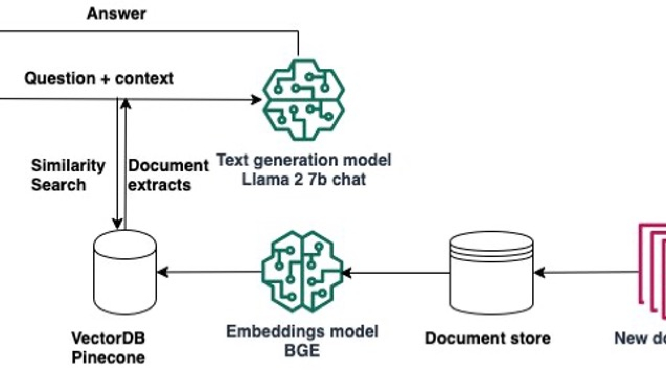
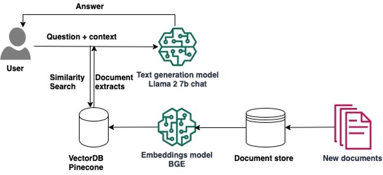
A typical RAG solution for knowledge retrieval from documents uses an embeddings model to convert the data from the data sources to embeddings and stores these embeddings in a vector database. When a user asks a question, it searches the vector database and retrieves documents that are most similar to the user’s query. Next, it combines the retrieved documents and the user’s query in an augmented prompt that is sent to the LLM for text generation. There are two models in this implementation: the embeddings model and the LLM that generates the final response.

In this post, we demonstrate how to use Amazon SageMaker Studio to build a RAG question answering solution.

Using notebooks for RAG-based question answering

Implementing RAG typically entails experimenting with various embedding models, vector databases, text generation models, and prompts, while also debugging your code until you achieve a functional prototype. Amazon SageMaker offers managed Jupyter notebooks equipped with GPU instances, enabling you to rapidly experiment during this initial phase without spinning up additional infrastructure. There are two options for using notebooks in SageMaker. The first option is fast launch notebooks available through SageMaker Studio. In SageMaker Studio, the integrated development environment (IDE) purpose-built for ML, you can launch notebooks that run on different instance types and with different configurations, collaborate with colleagues, and access additional purpose-built features for machine learning (ML). The second option is using a SageMaker notebook instance, which is a fully managed ML compute instance running the Jupyter Notebook app.

In this post, we present a RAG solution that augments the model’s knowledge with additional data from external knowledge sources to provide more accurate responses specific to a custom domain. We use a single SageMaker Studio notebook running on an ml.g5.2xlarge instance (1 A10G GPU) and Llama 2 7b chat hf, the fine-tuned version of Llama 2 7b, which is optimized for dialog use cases from Hugging Face Hub. We use two AWS Media & Entertainment Blog posts as the sample external data, which we convert into embeddings with the BAAI/bge-small-en-v1.5 embeddings. We store the embeddings in Pinecone, a vector-based database that offers high-performance search and similarity matching. We also discuss how to transition from experimenting in the notebook to deploying your models to SageMaker endpoints for real-time inference when you complete your prototyping. The same approach can be used with different models and vector databases.

Solution overview

The following diagram illustrates the solution architecture.

Implementing the solution consists of two high-level steps: developing the solution using SageMaker Studio notebooks, and deploying the models for inference.

Develop the solution using SageMaker Studio notebooks

Complete the following steps to start developing the solution:

1. Load the Llama-2 7b chat model from Hugging Face Hub in the notebook.
2. Create a PromptTemplate with LangChain and use it to create prompts for your use case.
3. For 1–2 example prompts, add relevant static text from external documents as prompt context and assess if the quality of the responses improves.
4. Assuming that the quality improves, implement the RAG question answering workflow:
   • Gather the external documents that can help the model better answer the questions in your use case.
   • Load the BGE embeddings model and use it to generate embeddings of these documents.
   • Store these embeddings in a Pinecone index.
   • When a user asks a question, perform a similarity search in Pinecone and add the content from the most similar documents to the prompt’s context.

Deploy the models to SageMaker for inference at scale

When you hit your performance goals, you can deploy the models to SageMaker to be used by generative AI applications:

1. Deploy the Llama-2 7b chat model to a SageMaker real-time endpoint.
2. Deploy the BAAI/bge-small-en-v1.5 embeddings model to a SageMaker real-time endpoint.
3. Use the deployed models in your question answering generative AI applications.

In the following sections, we walk you through the steps of implementing this solution in SageMaker Studio notebooks.

Prerequisites

To follow the steps in this post, you need to have an AWS account and an AWS Identity and Access Management (IAM) role with permissions to create and access the solution resources. If you are new to AWS, see Create a standalone AWS account.

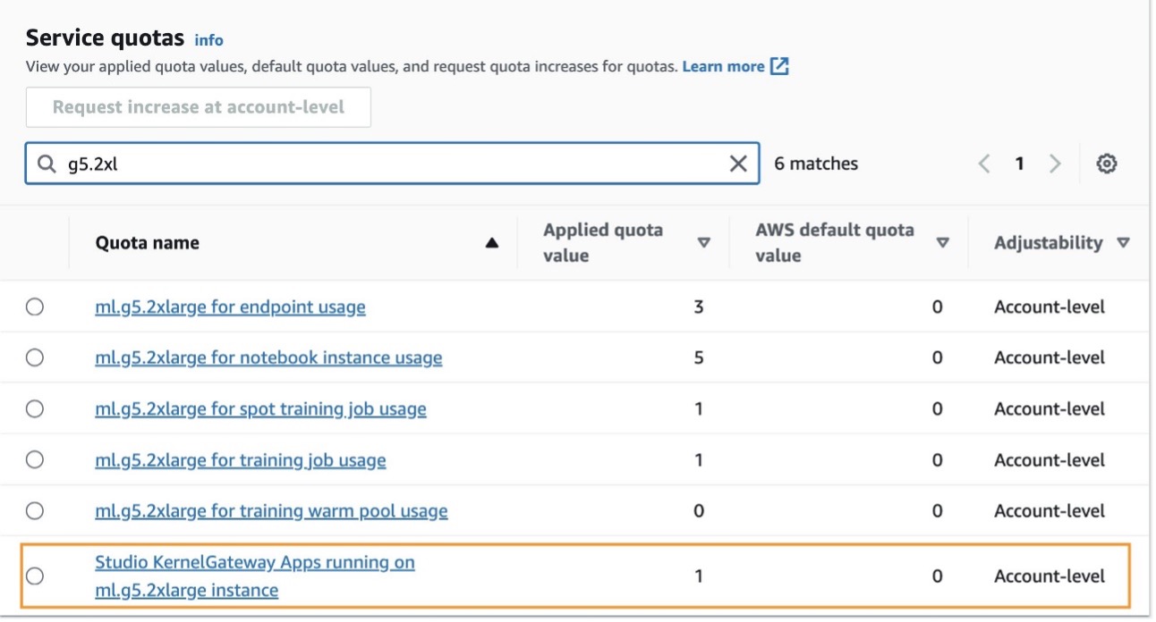
To use SageMaker Studio notebooks in your AWS account, you need a SageMaker domain with a user profile that has permissions to launch the SageMaker Studio app. If you are new to SageMaker Studio, the Quick Studio setup is the fastest way to get started. With a single click, SageMaker provisions the SageMaker domain with default presets, including setting up the user profile, IAM role, IAM authentication, and public internet access. The notebook for this post assumes an ml.g5.2xlarge instance type. To review or increase your quota, open the AWS Service Quotas console, choose AWS Services in the navigation pane, choose Amazon SageMaker, and refer to the value for Studio KernelGateway apps running on ml.g5.2xlarge instances.

After confirming your quota limit, you need to complete the dependencies to use Llama 2 7b chat.

Llama 2 7b chat is available under the Llama 2 license. To access Llama 2 on Hugging Face, you need to complete a few steps first:

1. Create a Hugging Face account if you don’t have one already.
2. Complete the form “Request access to the next version of Llama” on the Meta website.
3. Request access to Llama 2 7b chat on Hugging Face.

After you have been granted access, you can create a new access token to access models. To create an access token, navigate to the Settings page on the Hugging Face website.

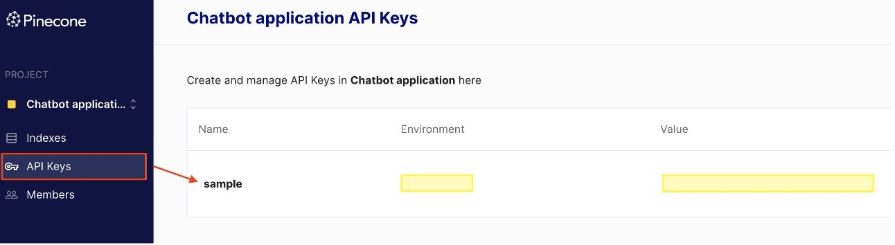
You need to have an account with Pinecone to use it as a vector database. Pinecone is available on AWS via the AWS Marketplace. The Pinecone website also offers the option to create a free account that comes with permissions to create a single index, which is sufficient for the purposes of this post. To retrieve your Pinecone keys, open the Pinecone console and choose API Keys.

Set up the notebook and environment

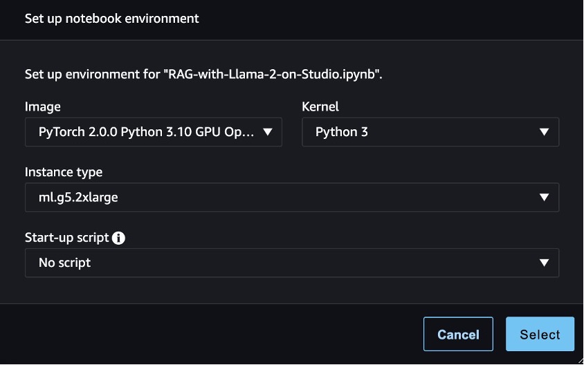
To follow the code in this post, open SageMaker Studio and clone the following GitHub repository. Next, open the notebook studio-local-gen-ai/rag/RAG-with-Llama-2-on-Studio.ipynb and choose the PyTorch 2.0.0 Python 3.10 GPU Optimized image, Python 3 kernel, and ml.g5.2xlarge as the instance type. If this is your first time using SageMaker Studio notebooks, refer to Create or Open an Amazon SageMaker Studio Notebook.

To set up the development environment, you need to install the necessary Python libraries, as demonstrated in the following code:

%%writefile requirements.txt
sagemaker>=2.175.0
transformers==4.33.0
accelerate==0.21.0
datasets==2.13.0
langchain==0.0.297
pypdf>=3.16.3
pinecone-client
sentence_transformers
safetensors>=0.3.3

!pip install -U -r requirements.txt

Load the pre-trained model and tokenizer

After you have imported the required libraries, you can load the Llama-2 7b chat model along with its corresponding tokenizers from Hugging Face. These loaded model artifacts are stored in the local directory within SageMaker Studio. This enables you to swiftly reload them into memory whenever you need to resume your work at a different time.

import torch

from transformers import (
	AutoTokenizer,
	LlamaTokenizer,
	LlamaForCausalLM,
	GenerationConfig,
	AutoModelForCausalLM
)
import transformers

tg_model_id = "meta-llama/Llama-2-7b-chat-hf" #the model id in Hugging Face
tg_model_path = f"./tg_model/{tg_model_id}" #the local directory where the model will be saved

tg_model = AutoModelForCausalLM.from_pretrained(tg_model_id, token=hf_access_token,do_sample=True, use_safetensors=True, device_map="auto", torch_dtype=torch.float16
tg_tokenizer = AutoTokenizer.from_pretrained(tg_model_id, token=hf_access_token)

tg_model.save_pretrained(save_directory=tg_model_path, from_pt=True)
tg_tokenizer.save_pretrained(save_directory=tg_model_path, from_pt=True)

Ask a question that requires up-to-date information

You can now start using the model and ask questions. Llama-2 chat models expect the prompt to adhere to the following format:

<s>[INST] <<SYS>>
system_prompt
<<SYS>>
{{ user_message }} [/INST]

You can use the PromptTemplate from LangChain to create a recipe based on the prompt format, so that you can easily create prompts going forward:

from langchain import PromptTemplate

template = """<s>[INST] <<SYS>>nYou are an assistant for question-answering tasks. You are helpful and friendly. Use the following pieces of retrieved context to answer the query. If you don't know the answer, you just say I don't know. Use three sentences maximum and keep the answer concise.
<<SYS>>n
{context}n
{question} [/INST]
"""
prompt_template = PromptTemplate( template=template, input_variables=['context','question'] )

Let’s ask the model a question that needs recent information from 2023. You can use LangChain and specifically the LLMChain type of chain and pass as parameters the LLM, the prompt template you created earlier, and the question:

question = "When can I visit the AWS M&E Customer Experience Center in New York City?"

tg_tokenizer.add_special_tokens( {"pad_token": "[PAD]"} )
tg_tokenizer.padding_side = "left"

tg_pipe = transformers.pipeline(task='text-generation', model=tg_model, tokenizer=tg_tokenizer, num_return_sequences=1, eos_token_id=tg_tokenizer.eos_token_id, pad_token_id=tg_tokenizer.eos_token_id, max_new_tokens=400, temperature=0.7)

from langchain.chains import LLMChain
from langchain.llms import HuggingFacePipeline

llm=HuggingFacePipeline(pipeline=tg_pipe, model_kwargs={'temperature':0.7})
llm_chain = LLMChain(llm=llm, prompt=prompt_template)
no_context_response = llm_chain.predict(context="", question=question)
print(no_context_response)

We get the following generated answer:

Thank you for reaching out! The AWS M&E Customer Experience Center in New York City is currently closed for visits due to the COVID-19 pandemic. However, you can check their official website or social media accounts for any updates on when the center will reopen. In the meantime, you can explore their virtual tours and resources available online.

Improve the answer by adding context to the prompt

The answer we generated is not entirely true. Let’s see if we can improve it by providing some context. You can add an extract from the post AWS announces new M&E Customer Experience Center in New York, which includes updates on the topic from 2023:

context = """Media and entertainment (M&E) customers continue to face challenges in creating more content, more quickly, and distributing it to more endpoints than ever before in their quest to delight viewers globally. Amazon Web Services (AWS), along with AWS Partners, have showcased the rapid evolution of M&E solutions for years at industry events like the National Association of Broadcasters (NAB) Show and the International Broadcast Convention (IBC). Until now, AWS for M&E technology demonstrations were accessible in this way just a few weeks out of the year. Customers are more engaged than ever before; they want to have higher quality conversations regarding user experience and media tooling. These conversations are best supported by having an interconnected solution architecture for reference. Scheduling a visit of the M&E Customer Experience Center will be available starting November 13th, please send an email to AWS-MediaEnt-CXC@amazon.com."""

Use the LLMChain again and pass the preceding text as context:

context_response = llm_chain.predict(context=context, question=question)
print(context_response)

The new response answers the question with up-to-date information:

You can visit the AWS M&E Customer Experience Center in New York City starting from November 13th. Please send an email to AWS-MediaEnt-CXC@amazon.com to schedule a visit.

We have confirmed that by adding the right context, the model’s performance is improved. Now you can focus your efforts on finding and adding the right context for the question asked. In other words, implement RAG.

Implement RAG question answering with BGE embeddings and Pinecone

At this juncture, you must decide on the sources of information to enhance the model’s knowledge. These sources could be internal webpages or documents within your organization, or publicly available data sources. For the purposes of this post and for the sake of simplicity, we have chosen two AWS Blog posts published in 2023:

• AWS announces new M&E Customer Experience Center in New York
• AWS Media Services awarded industry accolades

These posts are already available as PDF documents in the data project directory in SageMaker Studio for quick access. To divide the documents into manageable chunks, you can employ the RecursiveCharacterTextSplitter method from LangChain:

from langchain.text_splitter import RecursiveCharacterTextSplitter
from langchain.document_loaders import PyPDFDirectoryLoader

loader = PyPDFDirectoryLoader("./data/")

documents = loader.load()

text_splitter=RecursiveCharacterTextSplitter(
     chunk_size=1000,
     chunk_overlap=5
)
docs = text_splitter.split_documents(documents)

Next, use the BGE embeddings model bge-small-en created by the Beijing Academy of Artificial Intelligence (BAAI) that is available on Hugging Face to generate the embeddings of these chunks. Download and save the model in the local directory in Studio. We use fp32 so that it can run on the instance’s CPU.

em_model_name = "BAAI/bge-small-en"
em_model_path = f"./em-model"

from transformers import AutoModel
# Load model from HuggingFace Hub
em_model = AutoModel.from_pretrained(em_model_name,torch_dtype=torch.float32)
em_tokenizer = AutoTokenizer.from_pretrained(em_model_name,device="cuda")

# save model to disk
em_tokenizer.save_pretrained(save_directory=f"{em_model_path}/model",from_pt=True)
em_model.save_pretrained(save_directory=f"{em_model_path}/model",from_pt=True)
em_model.eval()

Use the following code to create an embedding_generator function, which takes the document chunks as input and generates the embeddings using the BGE model:

# Tokenize sentences
def tokenize_text(_input, device):
    return em_tokenizer(
        [_input], 
        padding=True, 
        truncation=True, 
        return_tensors='pt'
    ).to(device)

# Run embedding task as a function with model and text sentences as input
def embedding_generator(_input, normalize=True):
    # Compute token embeddings
    with torch.no_grad():
        embedded_output = em_model(
            **tokenize_text(
                _input, 
                em_model.device
            )
        )
        sentence_embeddings = embedded_output[0][:, 0]
        # normalize embeddings
        if normalize:
            sentence_embeddings = torch.nn.functional.normalize(
                sentence_embeddings, 
                p=2, 
                dim=1
            )
    
    return sentence_embeddings[0, :].tolist()
    
sample_sentence_embedding = embedding_generator(docs[0].page_content)
print(f"Embedding size of the document --->", len(sample_sentence_embedding))

In this post, we demonstrate a RAG workflow using Pinecone, a managed, cloud-native vector database that also offers an API for similarity search. You are free to rewrite the following code to use your preferred vector database.

We initialize a Pinecone python client and create a new vector search index using the embedding model’s output length. We use LangChain’s built-in Pinecone class to ingest the embeddings we created in the previous step. It needs three parameters: the documents to ingest, the embeddings generator function, and the name of the Pinecone index.

import pinecone
pinecone.init(
    api_key = os.environ["PINECONE_API_KEY"],
    environment = os.environ["PINECONE_ENV"]
)
#check if index already exists, if not we create it
index_name = "rag-index"
if index_name not in pinecone.list_indexes():
    pinecone.create_index(
        name=index_name,
        dimension=len(sample_sentence_embedding), ## 384 for bge-small-en 
        metric='cosine'
    )

#insert the embeddings
from langchain.vectorstores import Pinecone
vector_store = Pinecone.from_documents(
    docs,
    embedding_generator,
    index_name=index_name
)

With the Llama-2 7B chat model loaded into memory and the embeddings integrated into the Pinecone index, you can now combine these elements to enhance Llama 2’s responses for our question-answering use case. To achieve this, you can employ the LangChain RetrievalQA, which augments the initial prompt with the most similar documents from the vector store. By setting return_source_documents=True, you gain visibility into the exact documents used to generate the answer as part of the response, allowing you to verify the accuracy of the answer.

from langchain.chains import RetrievalQA
import textwrap

#helper method to improve the readability of the response
def print_response(llm_response):
    temp = [textwrap.fill(line, width=100) for line in llm_response['result'].split('n')]
    response = 'n'.join(temp)
    print(f"{llm_response['query']}n n{response}'n n Source Documents:")
    for source in llm_response["source_documents"]:
        print(source.metadata)

llm_qa_chain = RetrievalQA.from_chain_type(
    llm=llm, #the Llama-2 7b chat model
    chain_type='stuff',
    retriever=vector_store.as_retriever(search_kwargs={"k": 2}), # perform similarity search in Pinecone
    return_source_documents=True, #show the documents that were used to answer the question
    chain_type_kwargs={"prompt": prompt_template}
)
print_response(llm_qa_chain(question))

We get the following answer:

Q: When can I visit the AWS M&E Customer Experience Center in New York City?

A: I’m happy to help! According to the context, the AWS M&E Customer Experience Center in New York City will be available for visits starting on November 13th. You can send an email to AWS-MediaEnt-CXC@amazon.com to schedule a visit.’

Source Documents:

{‘page’: 4.0, ‘source’: ‘data/AWS announces new M&E Customer Experience Center in New York City _ AWS for M&E Blog.pdf’}

{‘page’: 2.0, ‘source’: ‘data/AWS announces new M&E Customer Experience Center in New York City _ AWS for M&E Blog.pdf’}

Let’s try a different question:

question2=" How many awards have AWS Media Services won in 2023?"
print_response(llm_qa_chain(question2))

We get the following answer:

Q: How many awards have AWS Media Services won in 2023?

A: According to the blog post, AWS Media Services have won five industry awards in 2023.’

Source Documents:

{‘page’: 0.0, ‘source’: ‘data/AWS Media Services awarded industry accolades _ AWS for M&E Blog.pdf’}

{‘page’: 1.0, ‘source’: ‘data/AWS Media Services awarded industry accolades _ AWS for M&E Blog.pdf’}

After you have established a sufficient level of confidence, you can deploy the models to SageMaker endpoints for real-time inference. These endpoints are fully managed and offer support for auto scaling.

SageMaker offers large model inference using Large Model Inference containers (LMIs), which we can utilize to deploy our models. These containers come equipped with pre-installed open source libraries like DeepSpeed, facilitating the implementation of performance-enhancing techniques such as tensor parallelism during inference. Additionally, they use DJLServing as a pre-built integrated model server. DJLServing is a high-performance, universal model-serving solution that offers support for dynamic batching and worker auto scaling, thereby increasing throughput.

In our approach, we use the SageMaker LMI with DJLServing and DeepSpeed Inference to deploy the Llama-2-chat 7b and BGE models to SageMaker endpoints running on ml.g5.2xlarge instances, enabling real-time inference. If you want to follow these steps yourself, refer to the accompanying notebook for detailed instructions.

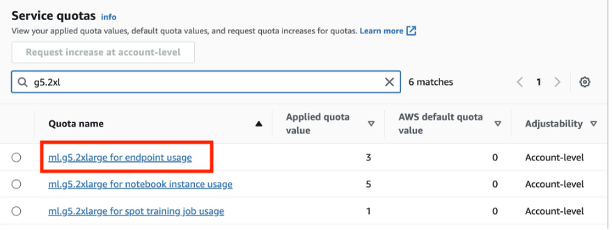
You will require two ml.g5.2xlarge instances for deployment. To review or increase your quota, open the AWS Service Quotas console, choose AWS Services in the navigation pane, choose Amazon SageMaker, and refer to the value for ml.g5.2xlarge for endpoint usage.

The following steps outline the process of deploying custom models for the RAG workflow on a SageMaker endpoint:

• Deploy the Llama-2 7b chat model to a SageMaker real-time endpoint running on an ml.g5.2xlarge instance for fast text generation.
• Deploy the BAAI/bge-small-en-v1.5 embeddings model to a SageMaker real-time endpoint running on an ml.g5.2xlarge instance. Alternatively, you can deploy your own embedding model.
• Ask a question and use the LangChain RetrievalQA to augment the prompt with the most similar documents from Pinecone, this time using the model deployed in the SageMaker real-time endpoint:

# convert your local LLM into SageMaker endpoint LLM
llm_sm_ep = SagemakerEndpoint(
    endpoint_name=tg_sm_model.endpoint_name, # <--- Your text-gen model endpoint name
    region_name=region,
    model_kwargs={
        "temperature": 0.05, 
        "max_new_tokens": 512
    },
    content_handler=content_handler,
)

llm_qa_smep_chain = RetrievalQA.from_chain_type(
    llm=llm_sm_ep,  # <--- This uses SageMaker Endpoint model for inference
    chain_type='stuff',
    retriever=vector_store.as_retriever(search_kwargs={"k": 2}),
    return_source_documents=True,
    chain_type_kwargs={"prompt": prompt_template}
)

• Use LangChain to verify that the SageMaker endpoint with the embedding model works as expected so that it can be used for future document ingestion:

response_model = smr_client.invoke_endpoint(
    EndpointName=em_sm_model.endpoint_name, <--- Your embedding model endpoint name
    Body=json.dumps({
        "text": "This is a sample text"
    }),
    ContentType="application/json",
)

outputs = json.loads(response_model["Body"].read().decode("utf8"))['outputs']

Clean up

Complete the following steps to clean up your resources:

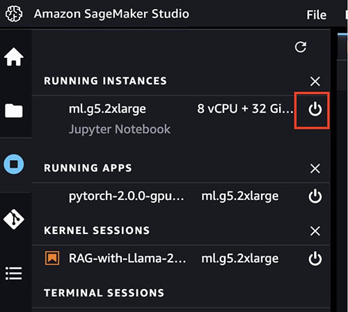
• When you have finished working in your SageMaker Studio notebook, make sure you shut down the ml.g5.2xlarge instance to avoid any charges by choosing the stop icon. You can also set up lifecycle configuration scripts to automatically shut down resources when they are not used.

• If you deployed the models to SageMaker endpoints, run the following code at the end of the notebook to delete the endpoints:

#delete your text generation endpoint
sm_client.delete_endpoint(
     EndpointName=tg_sm_model.endpoint_name
)
# delete your text embedding endpoint
sm_client.delete_endpoint(
      EndpointName=em_sm_model.endpoint_name
)

• Finally, run the following line to delete the Pinecone index:

pinecone.delete_index(index_name)

Conclusion

SageMaker notebooks provide a straightforward way to kickstart your journey with Retrieval Augmented Generation. They allow you to experiment interactively with various models, configurations, and questions without spinning up additional infrastructure. In this post, we showed how to enhance the performance of Llama 2 7b chat in a question answering use case using LangChain, the BGE embeddings model, and Pinecone. To get started, launch SageMaker Studio and run the notebook available in the following GitHub repo. Please share your thoughts in the comments section!

About the authors

Anastasia Tzeveleka is a Machine Learning and AI Specialist Solutions Architect at AWS. She works with customers in EMEA and helps them architect machine learning solutions at scale using AWS services. She has worked on projects in different domains including Natural Language Processing (NLP), MLOps and Low Code No Code tools.

Pranav Murthy is an AI/ML Specialist Solutions Architect at AWS. He focuses on helping customers build, train, deploy and migrate machine learning (ML) workloads to SageMaker. He previously worked in the semiconductor industry developing large computer vision (CV) and natural language processing (NLP) models to improve semiconductor processes. In his free time, he enjoys playing chess and traveling.

Read More

KT Corporation is one of the largest telecommunications providers in South Korea, offering a wide range of services including fixed-line telephone, mobile communication, and internet, and AI services. KT’s AI Food Tag is an AI-based dietary management solution that identifies the type and nutritional content of food in photos using a computer vision model. This vision model developed by KT relies on a model pre-trained with a large amount of unlabeled image data to analyze the nutritional content and calorie information of various foods. The AI Food Tag can help patients with chronic diseases such as diabetes manage their diets. KT used AWS and Amazon SageMaker to train this AI Food Tag model 29 times faster than before and optimize it for production deployment with a model distillation technique. In this post, we describe KT’s model development journey and success using SageMaker.

Introducing the KT project and defining the problem

The AI Food Tag model pre-trained by KT is based on the vision transformers (ViT) architecture and has more model parameters than their previous vision model to improve accuracy. To shrink the model size for production, KT is using a knowledge distillation (KD) technique to reduce the number of model parameters without significant impact to accuracy. With knowledge distillation, the pre-trained model is called a teacher model, and a lightweight output model is trained as a student model, as illustrated in the following figure. The lightweight student model has fewer model parameters than the teacher, which reduces memory requirements and allows for deployment on smaller, less expensive instances. The student maintains acceptable accuracy even though it’s smaller by learning from the outputs of the teacher model.

The teacher model remains unchanged during KD, but the student model is trained using the output logits of the teacher model as labels to calculate loss. With this KD paradigm, both the teacher and the student need to be on a single GPU memory for training. KT initially used two GPUs (A100 80 GB) in their internal, on-premises environment to train the student model, but the process took about 40 days to cover 300 epochs. To accelerate training and generate a student model in less time, KT partnered with AWS. Together, the teams significantly reduced model training time. This post describes how the team used Amazon SageMaker Training, the SageMaker Data Parallelism Library, Amazon SageMaker Debugger, and Amazon SageMaker Profiler to successfully develop a lightweight AI Food Tag model.

Building a distributed training environment with SageMaker

SageMaker Training is a managed machine learning (ML) training environment on AWS that provides a suite of features and tools to simplify the training experience and can be useful in distributed computing, as illustrated in the following diagram.

SageMaker customers can also access built-in Docker images with various pre-installed deep learning frameworks and the necessary Linux, NCCL, and Python packages for model training. Data scientists or ML engineers who want to run model training can do so without the burden of configuring training infrastructure or managing Docker and the compatibility of different libraries.

During a 1-day workshop, we were able to set up a distributed training configuration based on SageMaker within KT’s AWS account, accelerate KT’s training scripts using the SageMaker Distributed Data Parallel (DDP) library, and even test a training job using two ml.p4d.24xlarge instances. In this section, we describe KT’s experience working with the AWS team and using SageMaker to develop their model.

In the proof of concept, we wanted to speed up a training job by using the SageMaker DDP library, which is optimized for AWS infrastructure during distributed training. To change from PyTorch DDP to SageMaker DDP, you simply need to declare the torch_smddp package and change the backend to smddp, as shown in the following code:

import smdistributed.dataparallel.torch.torch_smddp

dist.init_process_group(backend='smddp',

rank=args.rank,

world_size=args.world_size)

To learn more about the SageMaker DDP library, refer to SageMaker’s Data Parallelism Library.

Analyzing the causes of slow training speed with the SageMaker Debugger and Profiler

The first step in optimizing and accelerating a training workload involves understanding and diagnosing where bottlenecks occur. For KT’s training job, we measured the training time per iteration of the data loader, forward pass, and backward pass:

Looking at the time in the standard output for each iteration, we saw that the backward pass’s run time fluctuated significantly from iteration to iteration. This variation is unusual and can impact total training time. To find the cause of this inconsistent training speed, we first tried to identify resource bottlenecks by utilizing the System Monitor (SageMaker Debugger UI), which allows you to debug training jobs on SageMaker Training and view the status of resources such as the managed training platform’s CPU, GPU, network, and I/O within a set number of seconds.

The SageMaker Debugger UI provides detailed and essential data that can help identifying and diagnose bottlenecks in a training job. Specifically, the CPU utilization line chart and CPU/GPU utilization heat map per instance tables caught our eye.

In the CPU utilization line chart, we noticed that some CPUs were being used 100%.

In the heat map (where darker colors indicate higher utilization), we noted that a few CPU cores had high utilization throughout the training, whereas GPU utilization wasn’t consistently high over time.

From here, we began to suspect that one of the reasons for the slow training speed was a CPU bottleneck. We reviewed the training script code to see if anything was causing the CPU bottleneck. The most suspicious part was the large value of num_workers in the data loader, so we changed this value to 0 or 1 to reduce CPU utilization. We then ran the training job again and checked the results.

The following screenshots show the CPU utilization line chart, GPU utilization, and heat map after mitigating the CPU bottleneck.

By simply changing num_workers, we saw a significant decrease in CPU utilization and an overall increase in GPU utilization. This was an important change that improved training speed significantly. Still, we wanted to see where we could optimize GPU utilization. For this, we used SageMaker Profiler.

SageMaker Profiler helps identify optimization clues by providing visibility into utilization by operations, including tracking GPU and CPU utilization metrics and kernel consumption of GPU/CPU within training scripts. It helps users understand which operations are consuming resources. First, to use SageMaker Profiler, you need to add ProfilerConfig to the function that invokes the training job using the SageMaker SDK, as shown in the following code:

from sagemaker import ProfilerConfig, Profiler

from sagemaker.debugger import (ProfilerRule, rule_configs)

rules=[ProfilerRule.sagemaker(rule_configs.ProfilerReport())]

profiler_config = ProfilerConfig(profile_params = Profiler(cpu_profiling_duration=3600))

from sagemaker.pytorch import PyTorch

region_name = 'us-west-2'

image_uri=f'763104351884.dkr.ecr.{region_name}.amazonaws.com/pytorch-training:2.0.0-gpu-py310-cu118-ubuntu20.04-sagemaker'

estimator = PyTorch(

entry_point='train.py',

source_dir='src',

role=role,

image_uri=image_uri,

instance_count=4,

instance_type='ml.p4d.24xlarge',

distribution={'smdistributed': {'dataparallel': {'enabled': True}}},

profiler_config=profiler_config,

hyperparameters=hyperparameters,

sagemaker_session=sagemaker_session,

)

In the SageMaker Python SDK, you have the flexibility to add the annotate functions for SageMaker Profiler to select code or steps in the training script that needs profiling. The following is an example of the code that you should declare for SageMaker Profiler in the training scripts:

import smppy

SMProf = smppy.SMProfiler.instance()

config = smppy.Config()

config.profiler = {

"EnableCuda": "1",

}

SMProf.configure(config)

SMProf.start_profiling()

…

with smppy.annotate("Forward"):

student_out = student_model(inp)

with smppy.annotate("Backward"):

loss.backward()

…

SMProf.stop_profiling()

After adding the preceding code, if you run a training job using the training scripts, you can get information about the operations consumed by the GPU kernel (as shown in the following figure) after the training runs for a period of time. In the case of KT’s training scripts, we ran it for one epoch and got the following results.

When we checked the top five operation consumption times of the GPU kernel among the results of SageMaker Profiler, we found that for the KT training script, the most time is consumed by the matrix product operation, which is a general matrix multiplication (GEMM) operation on GPUs. With this important insight from the SageMaker Profiler, we began investigating ways to accelerate these operations and improve GPU utilization.

Speeding up training time

We reviewed various ways to reduce computation time of matrix multiplication and applied two PyTorch functions.

Shard optimizer states with ZeroRedundancyOptimizer

If you look at the Zero Redundancy Optimizer (ZeRO), the DeepSpeed/ZeRO technique enables the training of a large model efficiently with better training speed by eliminating the redundancies in memory used by the model. ZeroRedundancyOptimizer in PyTorch uses the technique of sharding the optimizer state to reduce memory usage per a process in Distributed Data Parallel (DDP). DDP uses synchronized gradients in the backward pass so that all optimizer replicas iterate over the same parameters and gradient values, but instead of having all the model parameters, each optimizer state is maintained by sharding only for different DDP processes to reduce memory usage.

To use it, you can leave your existing Optimizer in optimizer_class and declare a ZeroRedundancyOptimizer with the rest of the model parameters and the learning rate as parameters.

student_optimizer = ZeroRedundancyOptimizer(

student_model.parameters(),

optimizer_class=torch.optim.AdamW,

lr=initial_lr

)

Automatic mixed precision

Automatic mixed precision (AMP) uses the torch.float32 data type for some operations and torch.bfloat16 or torch.float16 for others, for the convenience of fast computation and reduced memory usage. In particular, because deep learning models are typically more sensitive to exponent bits than fraction bits in their computations, torch.bfloat16 is equivalent to the exponent bits of torch.float32, allowing them to learn quickly with minimal loss. torch.bfloat16 only runs on instances with A100 NVIDIA architecture (Ampere) or higher, such as ml.p4d.24xlarge, ml.p4de.24xlarge, and ml.p5.48xlarge.

To apply AMP, you can declare torch.cuda.amp.autocast in the training scripts as shown in the code above and declare dtype as torch.bfloat16.

with torch.cuda.amp.autocast(dtype="torch.bfloat16"):

teacher = teacher_model(input_data)

student = student_model(input_data)

loss = loss(teacher, student, target)

loss.requires_grad_(True)

loss.backward()

student_optimizer.step()

student_optimizer.zero_grad(set_to_none=True)

Results in SageMaker Profiler

After applying the two functions to the training scripts and running a train job for one epoch again, we checked the top five operations consumption times for the GPU kernel in SageMaker Profiler. The following figure shows our results.

We can see that the GEMM operation, which was at the top of the list before applying the two Torch functions, has disappeared from the top five operations, replaced by the ReduceScatter operation, which typically occurs in distributed training.

Training speed results of the KT distilled model

We increased the training batch size by 128 more to account for the memory savings from applying the two Torch functions, resulting in a final batch size of 1152 instead of 1024. The training of the final student model was able to run 210 epochs per 1 day; the training time and speedup between KT’s internal training environment and SageMaker are summarized in the following table.

The scalability of AWS allowed us to complete the training job 29 times faster than before using 32 GPUs instead of 2 on premises. As a result, using more GPUs on SageMaker would have significantly reduced training time with no difference in overall training costs.

Conclusion

Park Sang-min (Vision AI Serving Technology Team Leader) from the AI2XL Lab in KT’s Convergence Technology Center commented on the collaboration with AWS to develop the AI Food Tag model:

“Recently, as there are more transformer-based models in the vision field, the model parameters and required GPU memory are increasing. We are using lightweight technology to solve this issue, and it takes a lot of time, about a month to learn once. Through this PoC with AWS, we were able to identify the resource bottlenecks with help of SageMaker Profiler and Debugger, resolve them, and then use SageMaker’s data parallelism library to complete the training in about one day with optimized model code on four ml.p4d.24xlarge instances.”

SageMaker helped save Sang-min’s team weeks of time in model training and development.

Based on this collaboration on the vision model, AWS and the SageMaker team will continue to collaborate with KT on various AI/ML research projects to improve model development and service productivity through applying SageMaker capabilities.

To learn more about related features in SageMaker, check out the following:

• Train machine learning models
• SageMaker’s Data Parallelism Library
• Use Amazon SageMaker Debugger to debug and improve model performance
• Use Amazon SageMaker Profiler to profile activities on AWS compute resources

About the authors

Youngjoon Choi, AI/ML Expert SA, has experienced enterprise IT in various industries such as manufacturing, high-tech, and finance as a developer, architect, and data scientist. He conducted research on machine learning and deep learning, specifically on topics like hyperparameter optimization and domain adaptation, presenting algorithms and papers. At AWS, he specializes in AI/ML across industries, providing technical validation using AWS services for distributed training/large scale models and building MLOps. He proposes and reviews architectures, aiming to contribute to the expansion of the AI/ML ecosystem.

Jung Hoon Kim is an account SA of AWS Korea. Based on experiences in applications architecture design, development and systems modeling in various industries such as hi-tech, manufacturing, finance and public sector, he is working on AWS Cloud journey and workloads optimization on AWS for enterprise customers.

Rock Sakong is a researcher at KT R&D. He has conducted research and development for the vision AI in various fields and mainly conducted facial attributes (gender/glasses, hats, etc.)/face recognition technology related to the face. Currently, he is working on lightweight technology for the vision models.

Manoj Ravi is a Senior Product Manager for Amazon SageMaker. He is passionate about building next-gen AI products and works on software and tools to make large-scale machine learning easier for customers. He holds an MBA from Haas School of Business and a Masters in Information Systems Management from Carnegie Mellon University. In his spare time, Manoj enjoys playing tennis and pursuing landscape photography.

Robert Van Dusen is a Senior Product Manager with Amazon SageMaker. He leads frameworks, compilers, and optimization techniques for deep learning training.

Read More