Streamlining ETL data processing at Talent.com with Amazon SageMaker

Streamlining ETL data processing at Talent.com with Amazon SageMaker

This post is co-authored by Anatoly Khomenko, Machine Learning Engineer, and Abdenour Bezzouh, Chief Technology Officer at Talent.com.

Established in 2011, Talent.com aggregates paid job listings from their clients and public job listings, and has created a unified, easily searchable platform. Covering over 30 million job listings across more than 75 countries and spanning various languages, industries, and distribution channels, Talent.com caters to the diverse needs of job seekers, effectively connecting millions of job seekers with job opportunities.

Talent.com’s mission is to facilitate global workforce connections. To achieve this, Talent.com aggregates job listings from various sources on the web, offering job seekers access to an extensive pool of over 30 million job opportunities tailored to their skills and experiences. In line with this mission, Talent.com collaborated with AWS to develop a cutting-edge job recommendation engine driven by deep learning, aimed at assisting users in advancing their careers.

To ensure the effective operation of this job recommendation engine, it is crucial to implement a large-scale data processing pipeline responsible for extracting and refining features from Talent.com’s aggregated job listings. This pipeline is able to process 5 million daily records in less than 1 hour, and allows for processing multiple days of records in parallel. In addition, this solution allows for a quick deployment to production. The primary source of data for this pipeline is the JSON Lines format, stored in Amazon Simple Storage Service (Amazon S3) and partitioned by date. Each day, this results in the generation of tens of thousands of JSON Lines files, with incremental updates occurring daily.

The primary objective of this data processing pipeline is to facilitate the creation of features necessary for training and deploying the job recommendation engine on Talent.com. It’s worth noting that this pipeline must support incremental updates and cater to the intricate feature extraction requirements necessary for the training and deployment modules essential for the job recommendation system. Our pipeline belongs to the general ETL (extract, transform, and load) process family that combines data from multiple sources into a large, central repository.

For further insights into how Talent.com and AWS collaboratively built cutting-edge natural language processing and deep learning model training techniques, utilizing Amazon SageMaker to craft a job recommendation system, refer to From text to dream job: Building an NLP-based job recommender at Talent.com with Amazon SageMaker. The system includes feature engineering, deep learning model architecture design, hyperparameter optimization, and model evaluation, where all modules are run using Python.

This post shows how we used SageMaker to build a large-scale data processing pipeline for preparing features for the job recommendation engine at Talent.com. The resulting solution enables a Data Scientist to ideate feature extraction in a SageMaker notebook using Python libraries, such as Scikit-Learn or PyTorch, and then to quickly deploy the same code into the data processing pipeline performing feature extraction at scale. The solution does not require porting the feature extraction code to use PySpark, as required when using AWS Glue as the ETL solution. Our solution can be developed and deployed solely by a Data Scientist end-to-end using only a SageMaker, and does not require knowledge of other ETL solutions, such as AWS Batch. This can significantly shorten the time needed to deploy the Machine Learning (ML) pipeline to production. The pipeline is operated through Python and seamlessly integrates with feature extraction workflows, rendering it adaptable to a wide range of data analytics applications.

Solution overview

Overview for ETL pipeline using SageMaker Processing

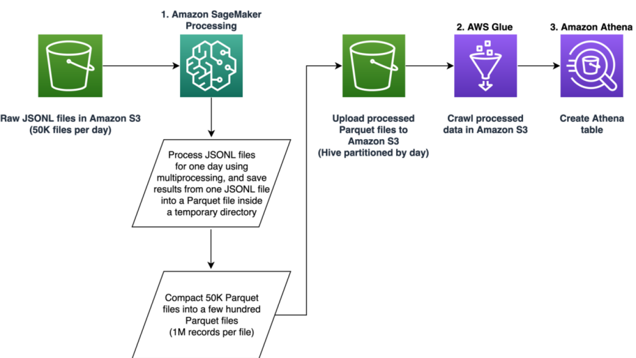
The pipeline is comprised of three primary phases:

  1. Utilize an Amazon SageMaker Processing job to handle raw JSONL files associated with a specified day. Multiple days of data can be processed by separate Processing jobs simultaneously.
  2. Employ AWS Glue for data crawling after processing multiple days of data.
  3. Load processed features for a specified date range using SQL from an Amazon Athena table, then train and deploy the job recommender model.

Process raw JSONL files

We process raw JSONL files for a specified day using a SageMaker Processing job. The job implements feature extraction and data compaction, and saves processed features into Parquet files with 1 million records per file. We take advantage of CPU parallelization to perform feature extraction for each raw JSONL file in parallel. Processing results of each JSONL file is saved into a separate Parquet file inside a temporary directory. After all of the JSONL files have been processed, we perform compaction of thousands of small Parquet files into several files with 1 million records per file. The compacted Parquet files are then uploaded into Amazon S3 as the output of the processing job. The data compaction ensures efficient crawling and SQL queries in the next stages of the pipeline.

The following is the sample code to schedule a SageMaker Processing job for a specified day, for example 2020-01-01, using the SageMaker SDK. The job reads raw JSONL files from Amazon S3 (for example from s3://bucket/raw-data/2020/01/01) and saves the compacted Parquet files into Amazon S3 (for example to s3://bucket/processed/table-name/day_partition=2020-01-01/).

### install dependencies 
%pip install sagemaker pyarrow s3fs awswrangler

import sagemaker
import boto3

from sagemaker.processing import FrameworkProcessor
from sagemaker.sklearn.estimator import SKLearn
from sagemaker import get_execution_role
from sagemaker.processing import ProcessingInput, ProcessingOutput

region = boto3.session.Session().region_name
role = get_execution_role()
bucket = sagemaker.Session().default_bucket()

### we use instance with 16 CPUs and 128 GiB memory
### note that the script will NOT load the entire data into memory during compaction
### depending on the size of individual jsonl files, larger instance may be needed
instance = "ml.r5.4xlarge"
n_jobs = 8  ### we use 8 process workers
date = "2020-01-01" ### process data for one day

est_cls = SKLearn
framework_version_str = "0.20.0"

### schedule processing job
script_processor = FrameworkProcessor(
    role=role,
    instance_count=1,
    instance_type=instance,
    estimator_cls=est_cls,
    framework_version=framework_version_str,
    volume_size_in_gb=500,
)

script_processor.run(
    code="processing_script.py", ### name of the main processing script
    source_dir="../src/etl/", ### location of source code directory

    ### our processing script loads raw jsonl files directly from S3
    ### this avoids long start-up times of the processing jobs,
    ### since raw data does not need to be copied into instance
    inputs=[], ### processing job input is empty

    outputs=[
        ProcessingOutput(destination="s3://bucket/processed/table-name/",
                         source="/opt/ml/processing/output"),
    ],
    arguments=[
        ### directory with job's output
        "--output", "/opt/ml/processing/output",

        ### temporary directory inside instance
        "--tmp_output", "/opt/ml/tmp_output",

        "--n_jobs", str(n_jobs), ### number of process workers
        "--date", date, ### date to process

        ### location with raw jsonl files in S3
        "--path", "s3://bucket/raw-data/",
    ],
    wait=False
)

The following code outline for the main script (processing_script.py) that runs the SageMaker Processing job is as follows:

import concurrent
import pyarrow.dataset as ds
import os
import s3fs
from pathlib import Path

### function to process raw jsonl file and save extracted features into parquet file  
from process_data import process_jsonl

### parse command line arguments
args = parse_args()

### we use s3fs to crawl S3 input path for raw jsonl files
fs = s3fs.S3FileSystem()
### we assume raw jsonl files are stored in S3 directories partitioned by date
### for example: s3://bucket/raw-data/2020/01/01/
jsons = fs.find(os.path.join(args.path, *args.date.split('-')))

### temporary directory location inside the Processing job instance
tmp_out = os.path.join(args.tmp_output, f"day_partition={args.date}")

### directory location with job's output
out_dir = os.path.join(args.output, f"day_partition={args.date}")

### process individual jsonl files in parallel using n_jobs process workers
futures=[]
with concurrent.futures.ProcessPoolExecutor(max_workers=args.n_jobs) as executor:
    for file in jsons:
        inp_file = Path(file)
        out_file = os.path.join(tmp_out, inp_file.stem + ".snappy.parquet")
        ### process_jsonl function reads raw jsonl file from S3 location (inp_file)
        ### and saves result into parquet file (out_file) inside temporary directory
        futures.append(executor.submit(process_jsonl, file, out_file))

    ### wait until all jsonl files are processed
    for future in concurrent.futures.as_completed(futures):
        result = future.result()

### compact parquet files
dataset = ds.dataset(tmp_out)

if len(dataset.schema) > 0:
    ### save compacted parquet files with 1MM records per file
    ds.write_dataset(dataset, out_dir, format="parquet", 
                     max_rows_per_file=1024 * 1024)

Scalability is a key feature of our pipeline. First, multiple SageMaker Processing jobs can be used to process data for several days simultaneously. Second, we avoid loading the entire processed or raw data into memory at once, while processing each specified day of data. This enables the processing of data using instance types that can’t accommodate a full day’s worth of data in primary memory. The only requirement is that the instance type should be capable of loading N raw JSONL or processed Parquet files into memory simultaneously, with N being the number of process workers in use.

Crawl processed data using AWS Glue

After all the raw data for multiple days has been processed, we can create an Athena table from the entire dataset by using an AWS Glue crawler. We use the AWS SDK for pandas (awswrangler) library to create the table using the following snippet:

import awswrangler as wr

### crawl processed data in S3
res = wr.s3.store_parquet_metadata(
    path='s3://bucket/processed/table-name/',
    database="database_name",
    table="table_name",
    dataset=True,
    mode="overwrite",
    sampling=1.0,
    path_suffix='.parquet',
)

### print table schema
print(res[0])

Load processed features for training

Processed features for a specified date range can now be loaded from the Athena table using SQL, and these features can then be used for training the job recommender model. For example, the following snippet loads one month of processed features into a DataFrame using the awswrangler library:

import awswrangler as wr

query = """
    SELECT * 
    FROM table_name
    WHERE day_partition BETWEN '2020-01-01' AND '2020-02-01' 
"""

### load 1 month of data from database_name.table_name into a DataFrame
df = wr.athena.read_sql_query(query, database='database_name')

Additionally, the use of SQL for loading processed features for training can be extended to accommodate various other use cases. For instance, we can apply a similar pipeline to maintain two separate Athena tables: one for storing user impressions and another for storing user clicks on these impressions. Using SQL join statements, we can retrieve impressions that users either clicked on or didn’t click on and then pass these impressions to a model training job.

Solution benefits

Implementing the proposed solution brings several advantages to our existing workflow, including:

  • Simplified implementation – The solution enables feature extraction to be implemented in Python using popular ML libraries. And, it does not require the code to be ported into PySpark. This streamlines feature extraction as the same code developed by a Data Scientist in a notebook will be executed by this pipeline.
  • Quick path-to-production – The solution can be developed and deployed by a Data Scientist to perform feature extraction at scale, enabling them to develop an ML recommender model against this data. At the same time, the same solution can be deployed to production by an ML Engineer with little modifications needed.
  • Reusability – The solution provides a reusable pattern for feature extraction at scale, and can be easily adapted for other use cases beyond building recommender models.
  • Efficiency – The solution offers good performance: processing a single day of the Talent.com’s data took less than 1 hour.
  • Incremental updates – The solution also supports incremental updates. New daily data can be processed with a SageMaker Processing job, and the S3 location containing the processed data can be recrawled to update the Athena table. We can also use a cron job to update today’s data several times per day (for example, every 3 hours).

We used this ETL pipeline to help Talent.com process 50,000 files per day containing 5 million records, and created training data using features extracted from 90 days of raw data from Talent.com—a total of 450 million records across 900,000 files. Our pipeline helped Talent.com build and deploy the recommendation system into production within only 2 weeks. The solution performed all ML processes including ETL on Amazon SageMaker without utilizing other AWS service. The job recommendation system drove an 8.6% increase in clickthrough rate in online A/B testing against a previous XGBoost-based solution, helping connect millions of Talent.com’s users to better jobs.

Conclusion

This post outlines the ETL pipeline we developed for feature processing for training and deploying a job recommender model at Talent.com. Our pipeline uses SageMaker Processing jobs for efficient data processing and feature extraction at a large scale. Feature extraction code is implemented in Python enabling the use of popular ML libraries to perform feature extraction at scale, without the need to port the code to use PySpark.

We encourage the readers to explore the possibility of using the pipeline presented in this blog as a template for their use-cases where feature extraction at scale is required. The pipeline can be leveraged by a Data Scientist to build an ML model, and the same pipeline can then be adopted by an ML Engineer to run in production. This can significantly reduce the time needed to productize the ML solution end-to-end, as was the case with Talent.com. The readers can refer to the tutorial for setting up and running SageMaker Processing jobs. We also refer the readers to view the post From text to dream job: Building an NLP-based job recommender at Talent.com with Amazon SageMaker, where we discuss deep learning model training techniques utilizing Amazon SageMaker to build Talent.com’s job recommendation system.


About the authors

Dmitriy BespalovDmitriy Bespalov is a Senior Applied Scientist at the Amazon Machine Learning Solutions Lab, where he helps AWS customers across different industries accelerate their AI and cloud adoption.

Yi XiangYi Xiang is a Applied Scientist II at the Amazon Machine Learning Solutions Lab, where she helps AWS customers across different industries accelerate their AI and cloud adoption.

Tong WangTong Wang is a Senior Applied Scientist at the Amazon Machine Learning Solutions Lab, where he helps AWS customers across different industries accelerate their AI and cloud adoption.

Anatoly KhomenkoAnatoly Khomenko is a Senior Machine Learning Engineer at Talent.com with a passion for natural language processing matching good people to good jobs.

Abdenour BezzouhAbdenour Bezzouh is an executive with more than 25 years experience building and delivering technology solutions that scale to millions of customers. Abdenour held the position of Chief Technology Officer (CTO) at Talent.com when the AWS team designed and executed this particular solution for Talent.com.

Yanjun QiYanjun Qi is a Senior Applied Science Manager at the Amazon Machine Learning Solution Lab. She innovates and applies machine learning to help AWS customers speed up their AI and cloud adoption.

Read More

FunSearch: Making new discoveries in mathematical sciences using Large Language Models

FunSearch: Making new discoveries in mathematical sciences using Large Language Models

In a paper published in Nature, we introduce FunSearch, a method for searching for “functions” written in computer code, and find new solutions in mathematics and computer science. FunSearch works by pairing a pre-trained LLM, whose goal is to provide creative solutions in the form of computer code, with an automated “evaluator”, which guards against hallucinations and incorrect ideas.Read More

FunSearch: Making new discoveries in mathematical sciences using Large Language Models

FunSearch: Making new discoveries in mathematical sciences using Large Language Models

In a paper published in Nature, we introduce FunSearch, a method for searching for “functions” written in computer code, and find new solutions in mathematics and computer science. FunSearch works by pairing a pre-trained LLM, whose goal is to provide creative solutions in the form of computer code, with an automated “evaluator”, which guards against hallucinations and incorrect ideas.Read More

‘Forza Horizon’ Races Over to GeForce NOW

‘Forza Horizon’ Races Over to GeForce NOW

This GFN Thursday is burning rubber with the latest Forza Horizon games from Microsoft Studios. Check them out on PC Game Pass.

Plus, give the gift of cloud gaming with the latest membership bundle, which includes a free, three-month PC Game Pass subscription with the purchase of a six-month GeForce NOW Ultimate membership.

It’s all part of an exciting week, with 13 new games joining the GeForce NOW library.

Zoom, Zoom

Jump into the driver’s seat in Forza Horizon 4 and Forza Horizon 5 from Playground Games and Microsoft Studios. Explore the critically acclaimed open-world racing games, featuring dynamic weather and seasons that can make or break even the most seasoned drivers.

Forza Horizon 4 on GeForce NOW
For-za cloud.

Race across beautiful, historical Great Britain in Forza Horizon 4. Ride solo or team up online with players from around the globe in a shared, open world. Collect, modify and drive over 450 cars from the Horizon car roster — plus, race, stunt, create and explore to become a Horizon Superstar.

Forza Horizon 5 on GeForce NOW
The ultimate “Horizon” adventure plays best on the ultimate cloud gaming service.

Clutch in, shift gears and head over to the vibrant open world of Mexico in Forza Horizon 5. Jump-start the week with limitless driving action in hundreds of the world’s greatest cars. Join a campaign with hundreds of challenges across varied terrains and climates, or head online for multiplayer action. Members can enjoy both titles in Steam and Forza Horizon 5 in PC Game Pass. Visit this Knowledgebase article for further details.

Stream every turn at GeForce quality on nearly any device and max out image resolution thanks to the cloud. Ultimate members can get in gear at up to 4K resolution and 120 frames per second for the most realistic driving experience.

The Ultimate Adventure

Minecraft Dungeons on GeForce NOW
What a blockhead.

Minecraft Dungeons from Mojang Studios and Xbox Game Studios is an immensely popular title that’s amassed over 25 million players and brings the thrill of classic dungeon crawlers to a whole new level.

Brave the dungeons alone or team up with a squad. Up to four players can battle together online or in couch co-op, making it a great game for group gatherings. Fight through action-packed, treasure-stuffed, wildly varied levels — all part of an epic quest to save the villagers and take down the evil Arch-Illager, preventing his army from controlling the Overworld.

Stream it on an Ultimate and Priority account for longer gaming sessions and faster access to GeForce RTX-powered servers. Venture forth across devices and play it on the big screen with NVIDIA SHIELD TV or on Samsung and LG smart TVs for the ultimate couch co-op experience.

Games, Games, Games

Pioneers of Pagonia on GeForce NOW
Be a pioneer of the cloud.

Time for some new games. Explore, discover and reunite the fantastical islands of Pagonia in Pioneers of Pagonia from Envision Entertainment. Build over 40 types of buildings, use more than 70 types of goods, manage widely branched production chains and get creative to establish a thriving economy.

Don’t miss the 13 newly supported games joining the GeForce NOW library this week:

  • Stellaris Nexus (New release on Steam, Dec. 12)
  • Tin Hearts (New release on Xbox, available PC Game Pass, Dec. 12)
  • Pioneers of Pagonia (New release on Steam, Dec. 13)
  • House Flipper 2 (New release on Steam, Dec. 14)
  • Soulslinger: Envoy of Death (New release on Steam, Dec. 14)
  • Escape the Backrooms (Steam)
  • Flashback 2 (Steam)
  • Forza Horizon 4 (Steam)
  • Forza Horizon 5 (Steam, Xbox, and available on PC Game Pass)
  • The Front (Steam)
  • Minecraft Dungeons (Steam, Xbox and available on PC Game Pass)
  • Primal Carnage: Extinction (Steam)
  • Universe Sandbox (Steam)

What are you planning to play this weekend? Let us know on Twitter or in the comments below.

Read More

Understanding GPU Memory 1: Visualizing All Allocations over Time

Understanding GPU Memory 1: Visualizing All Allocations over Time

During your time with PyTorch on GPUs, you may be familiar with this common error message:

torch.cuda.OutOfMemoryError: CUDA out of memory. Tried to allocate 512.00 MiB. GPU 0 has a total capacity of 79.32 GiB of which 401.56 MiB is free.

In this series, we show how to use memory tooling, including the Memory Snapshot, the Memory Profiler, and the Reference Cycle Detector to debug out of memory errors and improve memory usage.

Memory Timeline

The Memory Snapshot tool provides a fine-grained GPU memory visualization for debugging GPU OOMs. Captured memory snapshots will show memory events including allocations, frees and OOMs, along with their stack traces.

In a snapshot, each tensor’s memory allocation is color coded separately. The x axis is over time, and the y axis is the amount of GPU memory in MB. The snapshot is interactive, so we can observe the stack trace for any allocation by mousing over.

In this snapshot, there are 3 peaks showing the memory allocations over 3 training iterations. When looking at the peaks, it is easy to see the rise of memory in the forward pass and the fall during the backward pass as the gradients are computed. It is also possible to see that the program has the same pattern of memory use iteration to iteration. One thing that stands out is the many tiny spikes in memory, by mousing over them, we see that they are buffers used temporarily by convolution operators.

Capturing Memory Snapshots

The API to capture memory snapshots is fairly simple and available in torch.cuda.memory:

  • Start: torch.cuda.memory._record_memory_history(max_entries=100000)
  • Save: torch.cuda.memory._dump_snapshot(file_name)
  • Stop: torch.cuda.memory._record_memory_history(enabled=None)

Code Snippet (for full code sample, see Appendix A):

   # Start recording memory snapshot history, initialized with a buffer
   # capacity of 100,000 memory events, via the `max_entries` field.
   torch.cuda.memory._record_memory_history(
       max_entries=MAX_NUM_OF_MEM_EVENTS_PER_SNAPSHOT
   )

   # Run your PyTorch Model.
   # At any point in time, save a snapshot to file for later.
   for _ in range(5):
       pred = model(inputs)
       loss_fn(pred, labels).backward()
       optimizer.step()
       optimizer.zero_grad(set_to_none=True)

   # In this sample, we save the snapshot after running 5 iterations.
   #   - Save as many snapshots as you'd like.
   #   - Snapshots will save last `max_entries` number of memory events
   #     (100,000 in this example).
   try:
       torch.cuda.memory._dump_snapshot(f"{file_prefix}.pickle")
   except Exception as e:
       logger.error(f"Failed to capture memory snapshot {e}")

   # Stop recording memory snapshot history.
   torch.cuda.memory._record_memory_history(enabled=None)

To visualize the snapshot file, we have a tool hosted at https://pytorch.org/memory_viz. There, you can drag and drop your saved snapshot file and it will plot each allocation over time.

Memory Timeline

Alternatively, you can generate an HTML from a .pickle by using the script at pytorch/torch/cuda/_memory_viz.py, here is an example:

python torch/cuda/_memory_viz.py trace_plot snapshot.pickle -o snapshot.html

Debugging CUDA OOMs

Let’s look at how we can use the memory snapshot tool to answer:

  1. Why did a CUDA OOM happen?
  2. Where is the GPU Memory being used?

ResNet50 with a bug

We’ve taken a look at a properly working model in the first snapshot. Now, let’s take a look at a training example with a bug, see snapshot:

Memory Timeline

Notice how the second iteration uses far more memory than the first iteration. If this model were much larger, it could have CUDA OOM’d in the second iteration without much more insight into why.

Memory Timeline

When examining this snapshot further, we can clearly see that several tensors are staying alive from the first iteration to the second and later iterations. If we mouse over one of these tensors, it would show a stack trace suggesting that these were gradient tensors.

And indeed if we go to the code, we can see that it doesn’t clear the gradient tensors, when it could have cleared them before the forward.

Before:

        for _ in range(num_iters):
          pred = model(inputs)
          loss_fn(pred, labels).backward()
          optimizer.step()

After:

        for _ in range(num_iters):
          pred = model(inputs)
          loss_fn(pred, labels).backward()
          optimizer.step()
          # Add this line to clear grad tensors
          optimizer.zero_grad(set_to_none=True)

We can simply add an optimizer.zero_grad(set_to_none=True) instruction to clear the gradient tensors from iteration to iteration (more details about why we need to zero the gradients here: https://pytorch.org/tutorials/recipes/recipes/zeroing_out_gradients.html).

This is a simplification of a bug we’ve found in more complicated programs using this tool. We encourage you to try out the Memory Snapshot on your GPU memory problems and let us know how it goes.

ResNet50 after bug fix

After applying the fix, the snapshot seems to be clearing the gradients now.

Memory Timeline

We now have the snapshot of a properly working ResNet50 model. Try out the code yourself (see code sample in Appendix A).

But you may be wondering, why is there still an increase in memory after the first iteration? To answer this, let’s visit the Memory Profiler in the next section.

Categorized Memory Usage

The Memory Profiler is an added feature of the PyTorch Profiler that categorizes memory usage over time. We still rely on the Memory Snapshot for stack traces for deep dives into memory allocations.

To generate a memory timeline, here is a code snippet (full code sample in Appendix B):

   # Initialize the profiler context with record_shapes, profile_memory,
   # and with_stack set to True.
   with torch.profiler.profile(
       activities=[
           torch.profiler.ProfilerActivity.CPU,
           torch.profiler.ProfilerActivity.CUDA,
       ],
       schedule=torch.profiler.schedule(wait=0, warmup=0, active=6, repeat=1),
       record_shapes=True,
       profile_memory=True,
       with_stack=True,
       on_trace_ready=trace_handler,
   ) as prof:
       # Run the PyTorch Model inside the profile context.
       for _ in range(5):
           prof.step()
           with record_function("## forward ##"):
               pred = model(inputs)

           with record_function("## backward ##"):
               loss_fn(pred, labels).backward()

           with record_function("## optimizer ##"):
               optimizer.step()
               optimizer.zero_grad(set_to_none=True)

   # Construct the memory timeline HTML plot.
   prof.export_memory_timeline(f"{file_prefix}.html", device="cuda:0")

For further reference, see https://pytorch.org/docs/main/profiler.html.

The Memory Profiler automatically generates categories based on the graph of tensor operations recorded during profiling.

Memory Timeline

In this Memory Timeline collected using the Memory Profiler, we have the same training example as before. We can observe the gradients in blue are now being cleared from iteration to iteration. We can also notice that the optimizer state in yellow is allocated after the first iteration, and is kept constant for the rest of the job.

This optimizer state is the reason behind the increase of GPU memory from the first iteration to the second. Try out the code yourself (see code sample in Appendix B). The Memory Profiler helps to improve training memory understanding so that model authors can figure out which categories are using the most GPU memory.

Where can I find these tools?

We hope that these tools will greatly improve your ability to debug CUDA OOMs and to understand your memory usage by category.

The Memory Snapshot and the Memory Profiler are available in the v2.1 release of PyTorch as experimental features.

Feedback

We look forward to hearing from you about any enhancements, bugs or memory stories that our tools helped to solve! As always, please feel free to open new issues on PyTorch’s Github page.

We are also open to contributions from the OSS community, feel free to tag Aaron Shi and Zachary DeVito in any Github PRs for reviews.

Acknowledgements

Really appreciate the content reviewers, Mark Saroufim, Gregory Chanan, and Adnan Aziz for reviewing this post and improving its readability.

Appendix

Appendix A – ResNet50 Memory Snapshot Code Example

# (c) Meta Platforms, Inc. and affiliates. 
import logging
import socket
from datetime import datetime, timedelta

import torch

from torchvision import models

logging.basicConfig(
   format="%(levelname)s:%(asctime)s %(message)s",
   level=logging.INFO,
   datefmt="%Y-%m-%d %H:%M:%S",
)
logger: logging.Logger = logging.getLogger(__name__)
logger.setLevel(level=logging.INFO)

TIME_FORMAT_STR: str = "%b_%d_%H_%M_%S"

# Keep a max of 100,000 alloc/free events in the recorded history
# leading up to the snapshot.
MAX_NUM_OF_MEM_EVENTS_PER_SNAPSHOT: int = 100000

def start_record_memory_history() -> None:
   if not torch.cuda.is_available():
       logger.info("CUDA unavailable. Not recording memory history")
       return

   logger.info("Starting snapshot record_memory_history")
   torch.cuda.memory._record_memory_history(
       max_entries=MAX_NUM_OF_MEM_EVENTS_PER_SNAPSHOT
   )

def stop_record_memory_history() -> None:
   if not torch.cuda.is_available():
       logger.info("CUDA unavailable. Not recording memory history")
       return

   logger.info("Stopping snapshot record_memory_history")
   torch.cuda.memory._record_memory_history(enabled=None)

def export_memory_snapshot() -> None:
   if not torch.cuda.is_available():
       logger.info("CUDA unavailable. Not exporting memory snapshot")
       return

   # Prefix for file names.
   host_name = socket.gethostname()
   timestamp = datetime.now().strftime(TIME_FORMAT_STR)
   file_prefix = f"{host_name}_{timestamp}"

   try:
       logger.info(f"Saving snapshot to local file: {file_prefix}.pickle")
       torch.cuda.memory._dump_snapshot(f"{file_prefix}.pickle")
   except Exception as e:
       logger.error(f"Failed to capture memory snapshot {e}")
       return

# Simple Resnet50 example to demonstrate how to capture memory visuals.
def run_resnet50(num_iters=5, device="cuda:0"):
   model = models.resnet50().to(device=device)
   inputs = torch.randn(1, 3, 224, 224, device=device)
   labels = torch.rand_like(model(inputs))
   optimizer = torch.optim.SGD(model.parameters(), lr=1e-2, momentum=0.9)
   loss_fn = torch.nn.CrossEntropyLoss()

   # Start recording memory snapshot history
   start_record_memory_history()

   for _ in range(num_iters):
       pred = model(inputs)
       loss_fn(pred, labels).backward()
       optimizer.step()
       optimizer.zero_grad(set_to_none=True)

   # Create the memory snapshot file
   export_memory_snapshot()

   # Stop recording memory snapshot history
   stop_record_memory_history()

if __name__ == "__main__":
    # Run the resnet50 model
    run_resnet50()

Appendix B – ResNet50 Memory Profiler Code Example

# (c) Meta Platforms, Inc. and affiliates. 
import logging
import socket
from datetime import datetime, timedelta

import torch

from torch.autograd.profiler import record_function
from torchvision import models

logging.basicConfig(
   format="%(levelname)s:%(asctime)s %(message)s",
   level=logging.INFO,
   datefmt="%Y-%m-%d %H:%M:%S",
)
logger: logging.Logger = logging.getLogger(__name__)
logger.setLevel(level=logging.INFO)

TIME_FORMAT_STR: str = "%b_%d_%H_%M_%S"

def trace_handler(prof: torch.profiler.profile):
   # Prefix for file names.
   host_name = socket.gethostname()
   timestamp = datetime.now().strftime(TIME_FORMAT_STR)
   file_prefix = f"{host_name}_{timestamp}"

   # Construct the trace file.
   prof.export_chrome_trace(f"{file_prefix}.json.gz")

   # Construct the memory timeline file.
   prof.export_memory_timeline(f"{file_prefix}.html", device="cuda:0")

def run_resnet50(num_iters=5, device="cuda:0"):
   model = models.resnet50().to(device=device)
   inputs = torch.randn(1, 3, 224, 224, device=device)
   labels = torch.rand_like(model(inputs))
   optimizer = torch.optim.SGD(model.parameters(), lr=1e-2, momentum=0.9)
   loss_fn = torch.nn.CrossEntropyLoss()

   with torch.profiler.profile(
       activities=[
           torch.profiler.ProfilerActivity.CPU,
           torch.profiler.ProfilerActivity.CUDA,
       ],
       schedule=torch.profiler.schedule(wait=0, warmup=0, active=6, repeat=1),
       record_shapes=True,
       profile_memory=True,
       with_stack=True,
       on_trace_ready=trace_handler,
   ) as prof:
       for _ in range(num_iters):
           prof.step()
           with record_function("## forward ##"):
               pred = model(inputs)

           with record_function("## backward ##"):
               loss_fn(pred, labels).backward()

           with record_function("## optimizer ##"):
               optimizer.step()
               optimizer.zero_grad(set_to_none=True)

if __name__ == "__main__":
    # Warm up
    run_resnet50()
    # Run the resnet50 model
    run_resnet50()

Read More