We’re bringing Gemini to more Google productsRead More

We’re bringing Gemini to more Google productsRead More

We’re bringing Gemini to more Google productsRead More

We’re bringing Gemini to more Google productsRead More

We’re bringing Gemini to more Google productsRead More

 Bard is now known as Gemini, with a mobile app and an Advanced experience that gives you access to our most capable AI model, Ultra 1.0.Read More

 We’re bringing Gemini to more Google products. Bard will now be called Gemini, and you can access our most capable AI model, Ultra 1.0, in Gemini Advanced.Read More
In the first post of this three-part series, we presented a solution that demonstrates how you can automate detecting document tampering and fraud at scale using AWS AI and machine learning (ML) services for a mortgage underwriting use case.
In the second post, we discussed an approach to develop a deep learning-based computer vision model to detect and highlight forged images in mortgage underwriting.
In this post, we present a solution to automate mortgage document fraud detection using an ML model and business-defined rules with Amazon Fraud Detector.
We use Amazon Fraud Detector, a fully managed fraud detection service, to automate the detection of fraudulent activities. With an objective to improve fraud prediction accuracies by proactively identifying document fraud, while improving underwriting accuracies, Amazon Fraud Detector helps you build customized fraud detection models using a historical dataset, configure customized decision logic using the built-in rules engine, and orchestrate risk decision workflows with the click of a button.
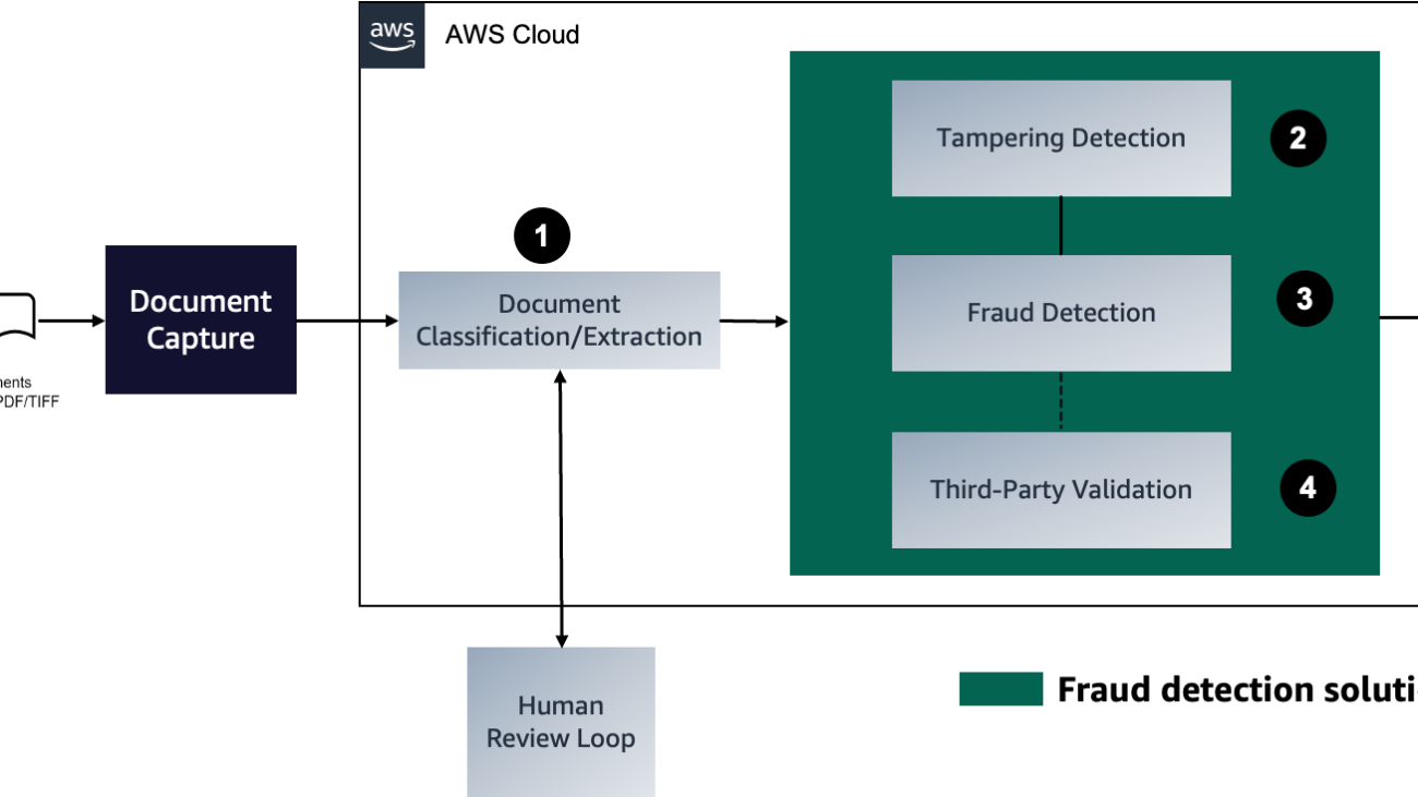
The following diagram represents each stage in a mortgage document fraud detection pipeline.

We will now be covering the third component of the mortgage document fraud detection pipeline. The steps to deploy this component are as follows:
The following are prerequisite steps for this solution:
EVENT_TIMESTAMP and EVENT_LABEL.After you have the custom historical data files to train a fraud detector model, create an S3 bucket and upload the data to the bucket.
The next step towards building and training a fraud detector model is to define the business activity (event) to evaluate for the fraud. Defining an event involves setting the variables in your dataset, an entity initiating the event, and the labels that classify the event.
Complete the following steps to define a docfraud event to detect document fraud, which is initiated by the entity applicant mortgage, referring to a new mortgage application:
docfraud as the event type name and, optionally, enter a description of the event.applicant_mortgage as the entity type name and, optionally, enter a description of the entity type.S3://your-bucket-name/example dataset filename.csv.Variables represent data elements that you want to use in a fraud prediction. These variables can be taken from the event dataset that you prepared for training your model, from your Amazon Fraud Detector model’s risk score outputs, or from Amazon SageMaker models. For more information about variables taken from the event dataset, see Get event dataset requirements using the Data models explorer.
fraud as the name. This label corresponds to the value that represents the fraudulent mortgage application in the example dataset.legit. This label corresponds to the value that represents the legitimate mortgage application in the example dataset.The following screenshot shows our event type details.

The following screenshot shows our variables.

The following screenshot shows our labels.

After you have loaded the historical data and selected the required options to train a model, complete the following steps to create a model:
mortgage_fraud_detection_model as the model’s name and an optional description of the model.docfraud. This is the event type that you created earlier.fraud, which corresponds to the value that represents fraudulent events in the example dataset.legit, which corresponds to the value that represents legitimate events in the example dataset.Amazon Fraud Detector creates a model and begins to train a new version of the model.
On the Model versions page, the Status column indicates the status of model training. Model training that uses the example dataset takes approximately 45 minutes to complete. The status changes to Ready to deploy after model training is complete.
After the model training is complete, Amazon Fraud Detector validates the model performance using 15% of your data that was not used to train the model and provides various tools, including a score distribution chart and confusion matrix, to assess model performance.
To view the model’s performance, complete the following steps:
sample_fraud_detection_model), then choose 1.0. This is the version Amazon Fraud Detector created of your model.
After you have reviewed the performance metrics of your trained model and are ready to use it generate fraud predictions, you can deploy the model:
sample_fraud_detection_model, and then choose the specific model version that you want to deploy. For this post, choose 1.0.On the Model versions page, the Status shows the status of the deployment. The status changes to Active when the deployment is complete. This indicates that the model version is activated and available to generate fraud predictions.
After you have deployed the model, you build a detector for the docfraud event type and add the deployed model. Complete the following steps:
fraud_detector for the detector name and, optionally, enter a description for the detector, such as my sample fraud detector.docfraud. This is the event that you created in earlier.After you have created the Amazon Fraud Detector model, you can use the Amazon Fraud Detector console or application programming interface (API) to define business-driven rules (conditions that tell Amazon Fraud Detector how to interpret model performance score when evaluating for fraud prediction). To align with the mortgage underwriting process, you may create rules to flag mortgage applications according to the risk levels associated and mapped as fraud, legitimate, or if a review is needed.
For example, you may want to automatically decline mortgage applications with a high fraud risk, considering parameters like tampered images of the required documents, missing documents like paystubs or income requirements, and so on. On the other hand, certain applications may need a human in the loop for making effective decisions.
Amazon Fraud Detector uses the aggregated value (calculated by combining a set of raw variables) and raw value (the value provided for the variable) to generate the model scores. The model scores can be between 0–1000, where 0 indicates low fraud risk and 1000 indicates high fraud risk.
To add the respective business-driven rules, complete the following steps:
$docdraud_insightscore >= 900high_risk rule available for use in your detector.
frauddecline$docdraud_insightscore >= 900low_risk rule with the following details:
legitapprove $docdraud_insightscore <= 500medium_risk rule with the following details:
review neededreview$docdraud_insightscore <= 900 and docdraud_insightscore >=500These values are examples used for this post. When you create rules for your own detector, use values that are appropriate for your model and use case.

After the rules-based actions have been triggered, you can deploy an Amazon Fraud Detector API to evaluate the lending applications and predict potential fraud. The predictions can be performed in a batch or real time.

If you already have a fraud detection model in SageMaker, you can integrate it with Amazon Fraud Detector for your preferred results.
This implies that you can use both SageMaker and Amazon Fraud Detector models in your application to detect different types of fraud. For example, your application can use the Amazon Fraud Detector model to assess the fraud risk of customer accounts, and simultaneously use your PageMaker model to check for account compromise risk.
To avoid incurring any future charges, delete the resources created for the solution, including the following:
This post walked you through an automated and customized solution to detect fraud in the mortgage underwriting process. This solution allows you to detect fraudulent attempts closer to the time of fraud occurrence and helps underwriters with an effective decision-making process. Additionally, the flexibility of the implementation allows you to define business-driven rules to classify and capture the fraudulent attempts customized to specific business needs.
For more information about building an end-to-end mortgage document fraud detection solution, refer to Part 1 and Part 2 in this series.
 Anup Ravindranath is a Senior Solutions Architect at Amazon Web Services (AWS) based in Toronto, Canada working with Financial Services organizations. He helps customers to transform their businesses and innovate on cloud.
 Vinnie Saini is a Senior Solutions Architect at Amazon Web Services (AWS) based in Toronto, Canada. She has been helping Financial Services customers transform on cloud, with AI and ML driven solutions laid on strong foundational pillars of Architectural Excellence.
The emergence of large language models (LLMs) has revolutionized the way people create text and interact with computing. However, these models are limited in ensuring the accuracy of the content they generate and enforcing strict compliance with specific formats, such as JSON and other computer programming languages. Additionally, LLMs that process information from multiple sources face notable challenges in preserving confidentiality and security. In sectors like healthcare, finance, and science, where information confidentiality and reliability are critical, the success of LLMs relies heavily on meeting strict privacy and accuracy standards. Current strategies to address these issues, such as constrained decoding and agent-based approaches, pose practical challenges, including significant performance costs or the need for direct model integration, which is difficult.
To make these approaches more feasible, we created the AI Controller Interface (AICI). The AICI goes beyond the standard “text-in/text-out” API for cloud-based tools with a “prompt-as-program” interface. It’s designed to allow user-level code to integrate with LLM output generation seamlessly in the cloud. It also provides support for existing security frameworks, application-specific functionalities, fast experimentation, and various strategies for improving accuracy, privacy, and adherence to specific formats. By providing granular-level access to the generative AI infrastructure, AICI allows for customized control over LLM processing, whether it’s run locally or in the cloud.
A lightweight virtual machine (VM), the AI Controller, sits atop this interface. AICI conceals the LLM processing engine’s specific implementation, providing the right mechanisms to enable developers and researchers to agilely and efficiently work with the LLM, allowing them to more easily develop and experiment. With features that allow for adjustments in decision-making processes, efficient memory use, handling multiple requests at once, and coordinating tasks simultaneously, users can finely tune the output, controlling it step by step.
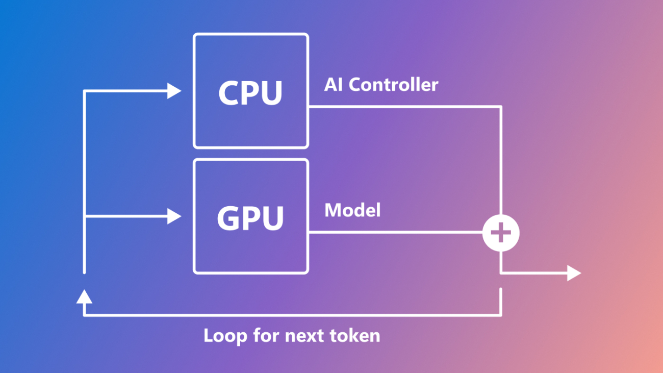
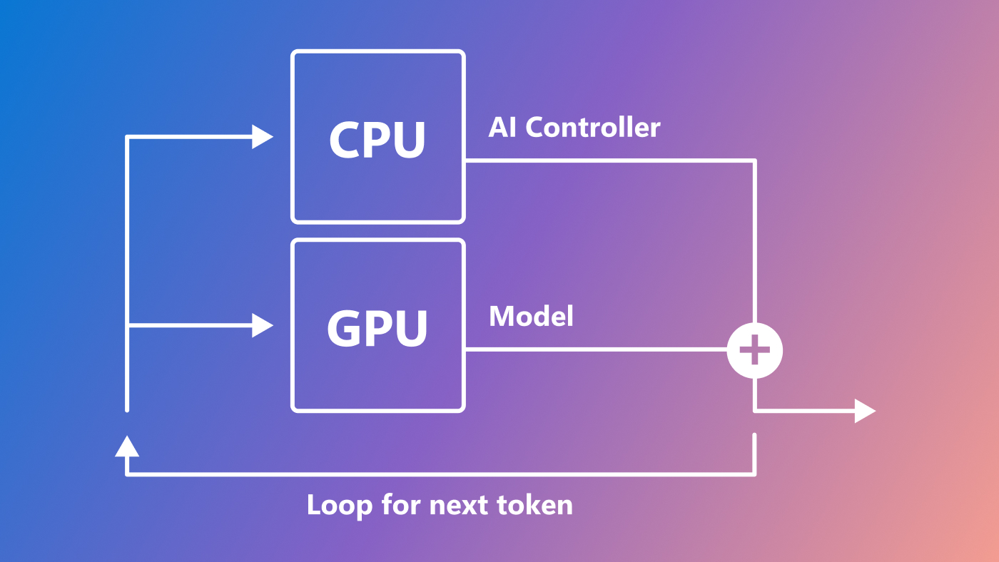
An individual user, tenant, or platform can develop the AI Controller program using a customizable interface designed for specific applications or prompt-completion tasks. The AICI is designed for the AI Controller to run on the CPU in parallel with model processing on the GPU, enabling advanced control over LLM behavior without impacting its performance. Additionally, multiple AI Controllers can run simultaneously. Figure 1 illustrates the AI Controller architecture.
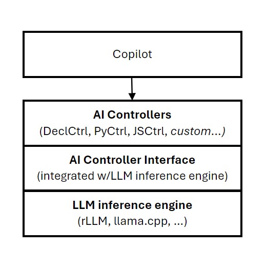
AI Controllers are implemented as WebAssembly VMs, most easily written as Rust programs. However, they can also be written in any language that can be compiled into or interpreted as WebAssembly. We have already developed several sample AI Controllers, available as open source (opens in new tab). These features provide built-in tools for controlled text creation, allowing for on-the-fly changes to initial instructions and the resulting text. They also enable efficient management of tasks that involve multiple stages or batch processing.
Let’s take an example to illustrate how the AI Controller impacts the output of LLMs. Suppose a user requests the completion of a task, such as solving a mathematical equation, with the expectation of receiving a numeric answer. The following program ensures the the LLM’s response is numeric. The process unfolds as follows:
1. Setup. The user or platform owner first sets up the AICI-enabled LLM engine and then deploys the provided AI Controller, DeclCtrl, to the cloud via a REST API.
2. Request. The user initiates LLM inference with a REST request specifying the AI Controller (DeclCtrl), and a JSON-formatted declarative program, such as the following example.
{"steps": [
    {"Fixed":{"text":"Please tell me what is 122.3*140.4?"}},
    {"Gen": {"rx":" ^(([1-9][0-9]*)|(([0-9]*).([0-9]*)))$"}}
]}
Once the server receives this request, it creates an instance of the requested DeclCtrl AI Controller and passes the declarative program into it. The AI Controller parses its input, initializes its internal state, and LLM inference begins.
3. Token generation. The server generates tokens sequentially, with the AICI making calls to the DeclCtrl AI Controller before, during, and after each token generation.
pre_process() is called before token generation. At this point, the AI Controller may stop generating (e.g., if it is complete), fork parallel generations, suspend, or continue.mid_process() is called during token generation and is the main entry point for computation in the AI Controller. During this call, the AI Controller can return logit biases to constrain generation, backtrack in the generation, or fast forward through a set of fixed or zero-entropy tokens. The mid_process() function runs in parallel with model inference on the GPU and its computation (e.g., of logit biases) is incorporated into the model’s token sampling on the GPU.post_process() is called once the model has generated the next token. Here, the AI Controller may, for example, perform simple bookkeeping, updating its state based on the sampled token.During these calls, the DeclCtrl AI Controller executes the necessary logic to ensure that the LLM generation conforms to the declarative program provided by the user. This ensures the LLM response is a numeric solution to the math problem.
4. Response. Once DeclCtrl completes its program, it assembles the results, which might include intermediate outputs, debug information, and computed variables. These can be returned as a final response or streamed to show progress. Finally, the AI Controller is deallocated.
Efficient constrained decoding
For Rust-based AI Controllers, we’ve developed an efficient way to check and enforce formatting rules (constraints) during text creation within the aici_abi library. This method involves using a special kind of search tree (called a trie) and checks based on patterns (regular expressions) or rules (context-free grammar) to ensure each piece of text follows specified constraints. This efficiency ensures rapid compliance-checking, enabling the program to seamlessly integrate with the GPU’s process without affecting performance.
While AI Controllers currently support mandatory formatting requirements, such as assigning negative infinity values to disallow invalid tokens, we anticipate that future versions will support more flexible guidance.
Information flow constraints
Furthermore, the AI Controller VM gives users the power to control the timing and manner by which prompts, background data, and intermediate text creations affect subsequent outputs. This is achieved through backtracking, editing, and prompt processing.
This functionality can be useful in a number of scenarios. For example, it allows users to selectively influence one part of a structured chain-of-thought process but not another. It can also be applied to preprocessing background data to remove irrelevant or potentially sensitive details before starting an LLM analysis. Currently, achieving this level of control requires multiple independent calls to LLMs.
Looking ahead
Our work with AICI has led to a successful implementation on a reference LLM serving engine (rLLM) and integrations with LLaMa.cpp. Currently, we’re working to provide a small set of standard AI Controllers for popular libraries like Guidance. In the near future, we plan to work with a variety of LLM infrastructures, and we’re excited to use the open-source ecosystem of LLM serving engines to integrate the AICI, providing portability for AI Controllers across environments.
Resources
Code, detailed descriptions of the AICI, and tutorials are available on GitHub (opens in new tab). We encourage developers and researchers to create and share their own custom AI Controllers.
The post AI Controller Interface: Generative AI with a lightweight, LLM-integrated VM appeared first on Microsoft Research.
New approach enables sustainable machine learning for remote-sensing applications.Read More

Welcome to Research Focus, a series of blog posts that highlights notable publications, events, code/datasets, new hires and other milestones from across the research community at Microsoft.

With a look back at the incredible changes of 2023 and a look ahead at the tangible advances to come, the inaugural Microsoft Research Forum explored bold new ideas and important issues in the era of general AI. Leaders from Microsoft Research, including the AI Frontiers team and the AI4Science lab, discussed the importance of openness and collaboration to enable successful and responsible AI research.
Peter Lee, CVP, Microsoft Research and Incubations, led off the discussion, followed by a panel exploring some of the biggest potential AI breakthroughs, along with challenges to overcome. This includes:
In the “lightning round,” Microsoft researchers explored current work to improve pretrained large language models, understand and evaluate foundation models, facilitate breakthroughs in molecular science, augment human decision making, and improve visual storytelling.
To learn more, check out this recap (opens in new tab) and browse the on-demand session replays (opens in new tab). Be sure to register for upcoming episodes (opens in new tab).
Spotlight: On-demand video
Explore how the transformer architecture, larger models and more data, and in-context learning have helped advance AI from perception to creation.
Transformer-based large language models (LLMs) have become a fixture in machine learning. Correspondingly, significant resources are allocated towards research to further advance this technology, typically resulting in models of increasing size that are trained on increasing amounts of data.
In a recent paper, The Truth is in There: Improving Reasoning in Language Models with Layer-Selective Rank Reduction, researchers from Microsoft demonstrate a surprising result: that it is possible to significantly improve LLM performance by selectively removing higher-order components of their constituent weight matrices. As covered in a Microsoft Research Forum lightning talk, this simple intervention—LAyer-SElective Rank reduction (LASER)—can be done on a model after training has been completed, and requires no additional parameters or data. In extensive experiments, the researchers demonstrate the generality of this finding across language models and datasets. They provide in-depth analyses offering insights into both when LASER is effective and the mechanism by which it operates.
Business intelligence tools make it easy to analyze large amounts of data. In these tools, top-k aggregation queries are used to summarize and identify important groups of data. These queries are usually processed by computing exact aggregates for all groups and then selecting the groups with the top-k aggregate values. However, this can be inefficient for high-cardinality large datasets, where intermediate results may not fit within the local cache of multi-core processors, leading to excessive data movement.
Researchers from Microsoft, in their recent paper: Cache-Efficient Top-k Aggregation over High Cardinality Large Datasets, introduce a new cache-conscious algorithm to address this. The algorithm efficiently computes exact top-k aggregates without fully processing all groups. Aggregation over large datasets requires multiple passes of data partitioning and repartitioning, thereby presenting a significant opportunity to reduce partitioning overhead for top-k aggregation queries. The algorithm leverages skewness in data distribution to select a small set of candidate groups for early aggregation. This helps eliminate many non-candidates group partitions through efficient partitioning techniques and coarse-grained statistics without computing exact aggregation. Empirical evaluation using both real-world and synthetic datasets demonstrate that the algorithm achieves a median speed-up of over 3x for monotonic aggregation functions and 1.4x for non-monotonic functions, compared to existing cache-conscious aggregation methods, across standard k value ranges (1 to 100).
The Association for Computing Machinery’s (ACM) annual fellows award recognizes people who make transformative contributions to computing science and technology. For 2023, the global organization named six researchers from Microsoft among its 68 award recipients.
Jianfeng Gao – VP and Distinguished Scientist
For contributions to machine learning for web search, natural language processing, and conversational systems
Sumit Gulwani – Partner Research Manager
For contributions to AI-assisted programming for developers, data scientists, end users, and students
Nicole Immorlica – Senior Principal Researcher
For contributions to economics and computation including market design, auctions, and social networks
Stefan Saroiu – Senior Principal Researcher
For contributions to memory security and trusted computing
Manik Varma – VP and Distinguished Scientist
For contributions to machine learning and its applications
Xing Xie – Senior Principal Research Manager
For contributions to spatial data mining and recommendation systems
The post Research Focus: Week of February 5, 2024 appeared first on Microsoft Research.