Revolutionize Customer Satisfaction with tailored reward models for your business on Amazon SageMaker

Revolutionize Customer Satisfaction with tailored reward models for your business on Amazon SageMaker

As more powerful large language models (LLMs) are used to perform a variety of tasks with greater accuracy, the number of applications and services that are being built with generative artificial intelligence (AI) is also growing. With great power comes responsibility, and organizations want to make sure that these LLMs produce responses that align with their organizational values and provide the same unique experience they always intended for their end-customers.

Evaluating AI-generated responses presents challenges. This post discusses techniques to align them with company values and build a custom reward model using Amazon SageMaker. By doing so, you can provide customized customer experiences that uniquely reflect your organization’s brand identity and ethos.

Challenges with out-of-the-box LLMs

Out-of-the-box LLMs provide high accuracy, but often lack customization for an organization’s specific needs and end-users. Human feedback varies in subjectivity across organizations and customer segments. Collecting diverse, subjective human feedback to refine LLMs is time-consuming and unscalable.

This post showcases a reward modeling technique to efficiently customize LLMs for an organization by programmatically defining rewards functions that capture preferences for model behavior. We demonstrate an approach to deliver LLM results tailored to an organization without intensive, continual human judgement. The techniques aim to overcome customization and scalability challenges by encoding an organization’s subjective quality standards into a reward model that guides the LLM to generate preferable outputs.

Objective vs. subjective human feedback

Not all human feedback is the same. We can categorize human feedback into two types: objective and subjective.

Any human being who is asked to judge the color of the following boxes would confirm that the left one is a white box and right one is a black box. This is objective, and there are no changes to it whatsoever.

Determining whether an AI model’s output is “great” is inherently subjective. Consider the following color spectrum. If asked to describe the colors on the ends, people would provide varied, subjective responses based on their perceptions. One person’s white may be another’s gray.

This subjectivity poses a challenge for improving AI through human feedback. Unlike objective right/wrong feedback, subjective preferences are nuanced and personalized. The same output could elicit praise from one person and criticism from another. The key is acknowledging and accounting for the fundamental subjectivity of human preferences in AI training. Rather than seeking elusive objective truths, we must provide models exposure to the colorful diversity of human subjective judgment.

Unlike traditional model tasks such as classification, which can be neatly benchmarked on test datasets, assessing the quality of a sprawling conversational agent is highly subjective. One human’s riveting prose is another’s aimless drivel. So how should we refine these expansive language models when humans intrinsically disagree on the hallmarks of a “good” response?

The key is gathering feedback from a diverse crowd. With enough subjective viewpoints, patterns emerge on engaging discourse, logical coherence, and harmless content. Models can then be tuned based on broader human preferences. There is a general perception that reward models are often associated only with Reinforcement Learning from Human Feedback (RLHF). Reward modeling, in fact, goes beyond RLHF, and can be a powerful tool for aligning AI-generated responses with an organization’s specific values and brand identity.

Reward modeling

You can choose an LLM and have it generate numerous responses to diverse prompts, and then your human labelers will rank those responses. It’s important to have diversity in human labelers. Clear labeling guidelines are critical. Without explicit criteria, judgments can become arbitrary. Useful dimensions include coherence, relevance, creativity, factual correctness, logical consistency, and more. Human labelers put these responses into categories and label them favorite to least favorite, as shown in the following example. This example showcases how different humans perceive these possible responses from the LLM in terms of their most favorite (labeled as 1 in this case) and least favorite (labeled as 3 in this case). Each column is labeled 1, 2, or 3 from each human to signify their most preferred and least preferred response from the LLM.

By compiling these subjective ratings, patterns emerge on what resonates across readers. The aggregated human feedback essentially trains a separate reward model on writing qualities that appeal to people. This technique of distilling crowd perspectives into an AI reward function is called reward modeling. It provides a method to improve LLM output quality based on diverse subjective viewpoints.

Solution overview

In this post, we detail how to train a reward model based on organization-specific human labeling feedback collected for various prompts tested on the base FM. The following diagram illustrates the solution architecture.

For more details, see the accompanying notebook.

Prerequisites

To successfully train a reward model, you need the following:

Launch SageMaker Studio

Complete the following steps to launch SageMaker Studio:

  1. On the SageMaker console, choose Studio in the navigation pane.
  2. On the Studio landing page, select the domain and user profile for launching Studio.
  3. Choose Open Studio.
  4. To launch SageMaker Studio, choose Launch personal Studio.

Let’s see how to create a reward model locally in a SageMaker Studio notebook environment by using a pre-existing model from the Hugging Face model hub.

Prepare a human-labeled dataset and train a reward model

When doing reward modeling, getting feedback data from humans can be expensive. This is because reward modeling needs feedback from other human workers instead of only using data collected during regular system use. How well your reward model behaves depends on the quality and amount of feedback from humans.

We recommend using AWS-managed offerings such as Amazon SageMaker Ground Truth. It offers the most comprehensive set of human-in-the-loop capabilities, allowing you to harness the power of human feedback across the machine learning (ML) lifecycle to improve the accuracy and relevancy of models. You can complete a variety of human-in-the-loop tasks with SageMaker Ground Truth, from data generation and annotation to model review, customization, and evaluation, either through a self-service or AWS-managed offering.

For this post, we use the IMDB dataset to train a reward model that provides a higher score for text that humans have labeled as positive, and a lower score for negative text.

We prepare the dataset with the following code:

def create_custom_dataset(raw_dataset):
    df = raw_dataset.to_pandas()
    negative_df = df[df['label']==0]
    positive_df = df[df['label']==1]
    negative_df = negative_df.drop(
        columns=['label']).rename(
        columns={'text': 'rejected'})
    # shuffle the data
    positive_df = positive_df.sample(
        frac=1, random_state=0).reset_index(
        drop=True).drop(columns=['label']).rename(
        columns={'text': 'chosen'})
    joined_df = negative_df.join(positive_df)

    def tokenize_fn(texts, max_length=args.seq_length):
        encoded = tokenizer(
            texts,
            padding='max_length',
            max_length=max_length,
            truncation=True,
            add_special_tokens=False,
        )
        return encoded

    rejected_encoded = tokenize_fn(joined_df.rejected.values.tolist())
    joined_df['rejected_input_ids'] = rejected_encoded['input_ids']
    joined_df['rejected_attention_mask'] = rejected_encoded['attention_mask']
    encoded_chosen = tokenize_fn(joined_df.chosen.values.tolist())
    joined_df['chosen_input_ids'] = encoded_chosen['input_ids']
    joined_df['chosen_attention_mask'] = encoded_chosen['attention_mask']
    
    train_dataset = Dataset.from_pandas(joined_df, preserve_index=False)
    
    return train_dataset.with_format("torch")

The following example shows a sample record from the prepared dataset, which includes references to rejected and chosen responses. We have also embedded the input ID and attention mask for the chosen and rejected responses.

{'rejected': "If only to avoid making this type of film in the future. This film is interesting as an experiment but tells no cogent story.<br /><br />One might feel virtuous for sitting thru it because it touches on so many IMPORTANT issues but it does so without any discernable motive. The viewer comes away with no new perspectives (unless one comes up with one while one's mind wanders, as it will invariably do during this pointless film).<br /><br />One might better spend one's time staring out a window at a tree growing.<br /><br />",
 'chosen': "This is a great movie. I love it more each time i watch. Most comedies can get pretty lame because you know all the gags, but mystery men has so much integrity in the writing and characterization that watching once again -- as Ben Stiller tears at the hood ornament of the limo, or Hank Azaria says good-bye to Louise Lasser, or Geoffrey Rush flashes his fuhrer choreography, or Tom Waits mumbles while he watches the news report, or Janeane Garofalo refuses a kiss from Paul Reubens -- is a pleasure. This is pitch perfect ensemble acting. The story develops directly and consistently, the action sequences are creative and not too dominant, all the set-ups payoff by the end. Seriously, if you've seen it and it's been a while, watch it again, and if you haven't then get started. You can't watch it again until you've seen it the first time. (Wes Studi, William H. Macy, the tryouts scene. Too much good stuff!)",
 'rejected_input_ids': tensor([1106,  129,    7,  ...,    1,    1,    1]),
 'rejected_attention_mask': tensor([1, 1, 1,  ..., 0, 0, 0]),
 'chosen_input_ids': tensor([713,  16,  10,  ...,   1,   1,   1]),
 'chosen_attention_mask': tensor([1, 1, 1,  ..., 0, 0, 0])}

Load the pre-trained model

In this case, we use the OPT-1.3b (Open Pre-trained Transformer Language Model) model in Amazon SageMaker JumpStart from Hugging Face. If you want to do all of the training locally on your notebook instead of distributed training, you need to use an instance with enough accelerator memory. We run the following training on a notebook running on ml.g4dn.xlarge instance type:

from transformers import( 
      AutoModelForSequenceClassification, 
      AutoTokenizer, 
      set_seed, 
      ) 
from datasets import Dataset, load_dataset 
import torch
       
model = AutoModelForSequenceClassification.from_pretrained( 
       'facebook/opt-1.3b',
       torch_dtype=torch.bfloat16, 
       device_map="auto", 
       num_labels=1, 
 )

Define the custom trainer function

In the following code snippet, we create a custom trainer that calculates how well a model is performing on a task:

from torch import nn 
from transformers import Trainer 
import torch.nn.functional as F 

class CustomTrainer(Trainer): 
def compute_loss(self, model, inputs, return_outputs=False): 

chosen_input_ids = inputs['chosen_input_ids'] chosen_attention_mask = inputs['chosen_attention_mask'] rejected_input_ids = inputs['rejected_input_ids'] rejected_attention_mask = inputs['rejected_attention_mask'] 
r_w = model(chosen_input_ids, chosen_attention_mask).logits 
r_l = model(rejected_input_ids, rejected_attention_mask).logits outputs = (r_w, r_l) 
loss = -F.logsigmoid(r_w - r_l).mean() 
return (loss, outputs) if return_outputs else loss

It compares the model’s results for two sets of input data: one set that was chosen and another set that was rejected. The trainer then uses these results to figure out how good the model is at distinguishing between the chosen and rejected data. This helps the trainer adjust the model to improve its performance on the task. The CustomTrainer class is used to create a specialized trainer that calculates the loss function for a specific task involving chosen and rejected input sequences. This custom trainer extends the functionality of the standard Trainer class provided by the transformers library, allowing for a tailored approach to handling model outputs and loss computation based on the specific requirements of the task. See the following code:

from transformers import TrainingArguments

training_args = TrainingArguments(output_dir="reward_model",
                                  overwrite_output_dir=True,
                                 do_train=True,
                                 do_eval=False,
                                 do_predict=False,
                                 evaluation_strategy="no",
                                 learning_rate=5e-5,
                                 num_train_epochs=1,
                                 per_device_train_batch_size=2,
                                 gradient_accumulation_steps=32,
                                 remove_unused_columns=False)
trainer = CustomTrainer( 
          model=model, 
          args=training_args, 
          train_dataset=train_dataset 
          )
trainer.train()
trainer.save_model()

The TrainingArguments in the provided code snippet are used to configure various aspects of the training process for an ML model. Let’s break down the purpose of each parameter, and how they can influence the training outcome:

  • output_dir – Specifies the directory where the trained model and associated files will be saved. This parameter helps organize and store the trained model for future use.
  • overwrite_output_dir – Determines whether to overwrite the output directory if it already exists. Setting this to True allows for reusing the same directory without manual deletion.
  • do_train – Indicates whether to perform training. If set to True, the model will be trained using the provided training dataset.
  • do_eval and do_predict – Control whether to perform evaluation and prediction tasks, respectively. In this case, both are set to False, meaning only training will be conducted.
  • evaluation_strategy – Defines when evaluation should be performed during training. Setting it to “no” means evaluation will not be done during training.
  • learning_rate – Specifies the learning rate for the optimizer, influencing how quickly or slowly the model learns from the data.
  • num_train_epochs – Sets the number of times the model will go through the entire training dataset during training. One epoch means one complete pass through all training samples.
  • per_device_train_batch_size – Determines how many samples are processed in each batch during training on each device (for example, GPU). A smaller batch size can lead to slower but more stable training.
  • gradient_accumulation_steps – Controls how often gradients are accumulated before updating the model’s parameters. This can help stabilize training with large batch sizes.
  • remove_unused_columns – Specifies whether unused columns in the dataset should be removed before processing, optimizing memory usage.

By configuring these parameters in the TrainingArguments, you can influence various aspects of the training process, such as model performance, convergence speed, memory usage, and overall training outcome based on your specific requirements and constraints.

When you run this code, it trains the reward model based on the numerical representation of subjective feedback you gathered from the human labelers. A trained reward model will give a higher score to LLM responses that humans are more likely to prefer.

Use the reward model to evaluate the base LLM

You can now feed the response from your LLM to this reward model, and the numerical score produced as output informs you of how well the response from the LLM is aligning to the subjective organization preferences that were embedded on the reward model. The following diagram illustrates this process. You can use this number as the threshold for deciding whether or not the response from the LLM can be shared with the end-user.

For example, let’s say we created an reward model to avoiding toxic, harmful, or inappropriate content. If a chatbot powered by an LLM produces a response, the reward model can then score the chatbot’s responses. Responses with scores above a pre-determined threshold are deemed acceptable to share with users. Scores below the threshold mean the content should be blocked. This lets us automatically filter chatbot content that doesn’t meet standards we want to enforce. To explore more, see the accompanying notebook.

Clean up

To avoid incurring future charges, delete all the resources that you created. Delete the deployed SageMaker models, if any, and stop the SageMaker Studio notebook you launched for this exercise.

Conclusion

In this post, we showed how to train a reward model that predicts a human preference score from the LLM’s response. This is done by generating several outputs for each prompt with the LLM, then asking human annotators to rank or score the responses to each prompt. The reward model is then trained to predict the human preference score from the LLM’s response. After the reward model is trained, you can use the reward model to evaluate the LLM’s responses against your subjective organizational standards.

As an organization evolves, the reward functions must evolve alongside changing organizational values and user expectations. What defines a “great” AI output is subjective and transforming. Organizations need flexible ML pipelines that continually retrain reward models with updated rewards reflecting latest priorities and needs. This space is continuously evolving: direct preference-based policy optimization, tool-augmented reward modeling, and example-based control are other popular alternative techniques to align AI systems with human values and goals.

We invite you to take the next step in customizing your AI solutions by engaging with the diverse and subjective perspectives of human feedback. Embrace the power of reward modeling to ensure your AI systems resonate with your brand identity and deliver the exceptional experiences your customers deserve. Start refining your AI models today with Amazon SageMaker and join the vanguard of businesses setting new standards in personalized customer interactions. If you have any questions or feedback, please leave them in the comments section.


About the Author

Dinesh Kumar Subramani is a Senior Solutions Architect based in Edinburgh, Scotland. He specializes in artificial intelligence and machine learning, and is member of technical field community with in Amazon. Dinesh works closely with UK Central Government customers to solve their problems using AWS services. Outside of work, Dinesh enjoys spending quality time with his family, playing chess, and exploring a diverse range of music.

Read More

Amazon Personalize launches new recipes supporting larger item catalogs with lower latency

Amazon Personalize launches new recipes supporting larger item catalogs with lower latency

Personalized customer experiences are essential for engaging today’s users. However, delivering truly personalized experiences that adapt to changes in user behavior can be both challenging and time-consuming. Amazon Personalize makes it straightforward to personalize your website, app, emails, and more, using the same machine learning (ML) technology used by Amazon, without requiring ML expertise. With the recipes—algorithms for specific uses cases—provided by Amazon Personalize, you can deliver a wide array of personalization, including product or content recommendations and personalized ranking.

Today, we are excited to announce the general availability of two advanced recipes in Amazon Personalize, User-Personalization-v2 and Personalized-Ranking-v2 (v2 recipes), which are built on the cutting-edge Transformers architecture to support larger item catalogs with lower latency.

In this post, we summarize the new enhancements, and guide you through the process of training a model and providing recommendations for your users.

Benefits of new recipes

The new recipes offer enhancements in scalability, latency, model performance, and functionality.

  • Enhanced scalability – The new recipes now support training with up to 5 million item catalogs and 3 billion interactions, empowering personalization for large catalogs and platforms with billions of usage events.
  • Lower latency – The lower inference latency and faster training times for large datasets of these new recipes can reduce the delay for your end-users.
  • Performance optimization – Amazon Personalize testing showed that v2 recipes improved recommendation accuracy by up to 9% and recommendation coverage by up to 1.8x compared to previous versions. A higher coverage means Amazon Personalize recommends more of your catalog.
  • Return item metadata in inference responses – The new recipes enable item metadata by default without extra charge, allowing you to return metadata such as genres, descriptions, and availability in inference responses. This can help you enrich recommendations in your user interfaces without extra work. If you use Amazon Personalize with generative AI, you can also feed the metadata into prompts. Providing more context to large language models can help them gain a deeper understanding of product attributes to generate more relevant content.
  • Highly automated operations – Our new recipes are designed to reduce your overhead for training and tuning the model. For example, Amazon Personalize simplifies training configuration and automatically selects the optimal settings for your custom models behind the scenes.

Solution overview

To use the User-Personalization-v2 and Personalized-Ranking-v2 recipes, you first need to set up Amazon Personalize resources. Create your dataset group, import your data, train a solution version, and deploy a campaign. For full instructions, see Getting started.

For this post, we follow the Amazon Personalize console approach to deploy a campaign. Alternatively, you can build the entire solution using the SDK approach. You can also get batch recommendations with an asynchronous batch flow. We use the MovieLens public dataset and User-Personalization-v2 recipe to show you the workflow.

Prepare the dataset

Complete the following steps to prepare your dataset:

  1. Create a dataset group. Each dataset group can contain up to three datasets: users, items, and interactions, with the interactions dataset being mandatory for User-Personalization-v2 and Personalized-Ranking-v2.
  2. Create an interactions dataset using a schema.
  3. Import the interactions data to Amazon Personalize from Amazon Simple Storage Service (Amazon S3).

Train a model

After the dataset import job is complete, you can analyze data before training. Amazon Personalize Data analysis shows you statistics about your data as well as actions you can take to meet training requirements and improve recommendations.

Now you’re ready to train your model.

  1. On the Amazon Personalize console, choose Dataset groups in the navigation pane.
  2. Choose your dataset group.
  3. Choose Create solutions.
  4. For Solution name, enter your solution name.
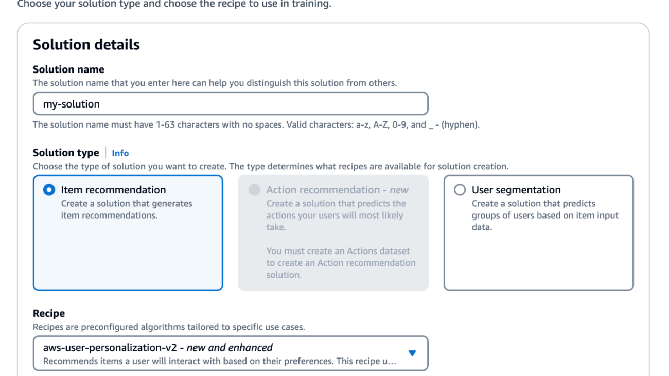
  5. For Solution type, select Item recommendation.
  6. For Recipe, choose the new aws-user-personalization-v2 recipe.
  7. In the Training configuration section, for Automatic training, select Turn on to maintain the effectiveness of your model by retraining it on a regular cadence.
  8. Under Hyperparameter configuration, select Apply recency bias. Recency bias determines whether the model should give more weight to the most recent item interactions data in your interactions dataset.
  9. Choose Create solution.

If you turned on automatic training, Amazon Personalize will automatically create your first solution version. A solution version refers to a trained ML model. When a solution version is created for the solution, Amazon Personalize trains the model backing the solution version based on the recipe and training configuration. It can take up to 1 hour for the solution version creation to start.

  1. Under Custom resources in the navigation pane, choose Campaigns.
  2. Choose Create campaign.

A campaign deploys a solution version (trained model) to generate real-time recommendations. Campaigns created with solutions trained on v2 recipes are automatically opted-in to include item metadata in recommendation results. You can choose metadata columns during an inference call.

  1. Provide your campaign details and create your campaign.

Get recommendations

After you create or update your campaign, you can get a recommended list of items that users are more likely to interact with, sorted from highest to lowest.

  1. Select the campaign and View details.
  2. In the Test campaign results section, enter the User ID and choose Get recommendations.

The following table shows a recommendation result for a user that includes the recommended items, relevance score, and item metadata (Title and Genre).

Your User-Personalization-v2 campaign is now ready to feed into your website or app and personalize the journey of each of your customers.

Clean up

Make sure you clean up any unused resources you created in your account while following the steps outlined in this post. You can delete campaigns, datasets, and dataset groups via the Amazon Personalize console or using the Python SDK.

Conclusion

The new Amazon Personalize User-Personalization-v2 and Personalized-Ranking-v2 recipes take personalization to the next level with support of larger item catalogs, reduced latency, and optimized performance. For more information about Amazon Personalize, see the Amazon Personalize Developer Guide.


About the Authors

Jingwen Hu is a Senior Technical Product Manager working with AWS AI/ML on the Amazon Personalize team. In her spare time, she enjoys traveling and exploring local food.

Daniel Foley is a Senior Product Manager for Amazon Personalize. He is focused on building applications that leverage artificial intelligence to solve our customers’ largest challenges. Outside of work, Dan is an avid skier and hiker.

Pranesh Anubhav is a Senior Software Engineer for Amazon Personalize. He is passionate about designing machine learning systems to serve customers at scale. Outside of his work, he loves playing soccer and is an avid follower of Real Madrid.

Tianmin Liu is a senior software engineer working for Amazon personalize. He focuses on developing recommender systems at scale using various machine learning algorithms. In his spare time, he likes playing video games, watching sports, and playing the piano.

Abhishek Mangal is a software engineer working for Amazon Personalize. He works on developing recommender systems at scale using various machine learning algorithms. In his spare time, he likes to watch anime and believes One Piece is the greatest piece of storytelling in recent history.

Yifei Ma is a Senior Applied Scientist at AWS AI Labs working on recommender systems. His research interests lie in active learning, generative models, time series analysis, and online decision-making. Outside of work, he is an aviation enthusiast.

Hao Ding is a Senior Applied Scientist at AWS AI Labs and is working on advancing the recommender system for Amazon Personalize. His research interests lie in recommendation foundation models, Bayesian deep learning, large language models, and their applications in recommendation.

Rishabh Agrawal is a Senior Software Engineer working on AI services at AWS. In his spare time, he enjoys hiking, traveling and reading.

Read More

Get started with Amazon Titan Text Embeddings V2: A new state-of-the-art embeddings model on Amazon Bedrock

Get started with Amazon Titan Text Embeddings V2: A new state-of-the-art embeddings model on Amazon Bedrock

Embeddings are integral to various natural language processing (NLP) applications, and their quality is crucial for optimal performance. They are commonly used in knowledge bases to represent textual data as dense vectors, enabling efficient similarity search and retrieval. In Retrieval Augmented Generation (RAG), embeddings are used to retrieve relevant passages from a corpus to provide context for language models to generate informed, knowledge-grounded responses. Embeddings also play a key role in personalization and recommendation systems by representing user preferences, item characteristics, and historical interactions as vectors, allowing calculation of similarities for personalized recommendations based on user behavior and item embeddings. As new embedding models are released with incremental quality improvements, organizations must weigh the potential benefits against the associated costs of upgrading, considering factors like computational resources, data reprocessing, integration efforts, and projected performance gains impacting business metrics.

In September of 2023, we announced the launch of Amazon Titan Text Embeddings V1, a multilingual text embeddings model that converts text inputs like single words, phrases, or large documents into high-dimensional numerical vector representations. Since then, many of our customers have used the V1 model, which supported over 25 languages, with an input up to 8,192 tokens and outputs vector of 1,536 dimensions for high accuracy and low latency. The model was made available as a serverless offering via Amazon Bedrock, simplifying embedding generation and integration with downstream applications. We published a follow-up post on January 31, 2024, and provided code examples using AWS SDKs and LangChain, showcasing a Streamlit semantic search app.

Today, we are happy to announce Amazon Titan Text Embeddings V2, our second-generation embeddings model for Amazon Bedrock. The new model is optimized for the most common use cases we see with many of our active customers, including RAG, multi-language, and code embedding use cases. The following table summarizes the key differences compared to V1.

Feature Amazon Titan Text Embeddings V1 Amazon Titan Text Embeddings V2
Output dimension support 1536 256, 512, 1024
Language support 25+ 100+
Unit vector normalization support No Yes
Price per million tokens $0.10 $0.02 per 1 million tokens, or $0.00002 per 1,000 tokens

With these new features, we expect many more customers choosing Amazon Titan Text Embeddings V2 to build common generative artificial intelligence (AI) applications. In this post, we discuss the benefits of the V2 model, how to conduct your own evaluation of the model, and how to migrate to using the new model.

Let’s dig in!

Benefits of Amazon Titan Text Embeddings V2

Amazon Titan Text Embeddings V2 is the second-generation embedding model for Amazon Bedrock, optimized for some of the most common customer use cases we have seen with our customers. Some of the key features include:

  • Optimized for RAG solutions
  • Flexible embedding sizes
  • Improved multilingual support and code

Embeddings have become an integral part of various NLP applications, and their quality is crucial for achieving optimal performance.

The large language model (LLM) landscape is rapidly evolving, with leading providers offering increasingly powerful and versatile embedding models. Although incremental improvements in embedding quality may seem modest at the high level, the actual benefits can be significant for specific use cases. For example, in a recommendation system for a large ecommerce platform, a modest increase in recommendation accuracy could translate into significant additional revenue.

A common way to select an embedding model (or any model) is to look at public benchmarks; an accepted benchmark for measuring embedding quality is the MTEB leaderboard. The Massive Text Embedding Benchmark (MTEB) evaluates text embedding models across a wide range of tasks and datasets. MTEB encompasses 8 different embedding tasks, covering a total of 58 datasets and 112 languages. In this benchmark, 33 different text embedding models were evaluated on the MTEB tasks. A key finding from the benchmark was that no single text embedding method emerged as the clear leader across all tasks and datasets. Each model exhibited strengths and weaknesses depending on the specific embedding task and data characteristics. This highlights the need for continued research into developing more versatile and robust text embedding techniques that can perform well across diverse use cases and language domains.

Although this is a useful benchmark, we caution our enterprise customers with the following considerations:

  • Although the MTEB leaderboard is widely recognized, it provides only a partial assessment by focusing solely on accuracy metrics and overlooking crucial practical factors like inference latency and model capabilities. The leaderboard rankings combine and compare embedding models across different vector dimensions, making direct and fair model comparisons challenging.
  • Additionally, the leaders on this accuracy-centric leaderboard change frequently as new models are continually introduced, providing a shifting and incomplete perspective on practical model performance trade-offs that real-world applications must consider beyond just accuracy numbers.
  • Lastly, costs need to be weighed against the expected benefits and performance improvements in the specific use case. A small gain in accuracy may not justify the significant overhead and opportunity costs of transitioning embeddings models, especially in large-scale, business-critical applications. Enterprises should perform a rigorous cost-benefit analysis to make sure the projected performance uplift from an updated embeddings model provides sufficient return on investment (ROI) to offset the migration costs and operational disruption.

In summary, start with evaluating the benchmark scores, but don’t decide until you have done your own due diligence.

Benchmark results

The Amazon Titan Text Embeddings V2 model has the ability to output embeddings of various size. This implies that if you use a lower size, you’ll reduce your memory footprint, which will translate directly into cost savings. The default size is 1024, compared to V1, which is an 1536 output size, implying a direct cost reduction of approximately 33%, which translates into savings given the cost of a RAG solution has a major component in the form of a vector databases. In our internal testing, we found that using the 256-output token resulted in only about 3.24% accuracy loss while translating to a four times saving due to size reduction. Running our evaluation on MTEB datasets, we found Amazon Titan Text Embeddings V2 to perform competitively with scores like 57.5 on reranking tasks, for example. With the model trained on over 100 languages, it’s no surprise the model achieves scores like 55 on the MIRACL multilingual dataset and has an overall weighted average MTEB score of 60.37. Full MTEB scores are available on the MTEB leaderboard.

However, we strongly encourage you to run your own benchmarks with your own dataset to understand the operational metrics. A sample notebook showing how to run the benchmarks against the MTEB datasets is hosted here. The key steps involved are:

  1. Choose a representative set of data to embed and keywords to search.
  2. Use the Amazon Titan Text Embeddings V2 model to embed your data and keywords, adjusting the chunk size and overlap as needed.
  3. Carry out a similarity search using your preferred vector comparison method (such as Euclidean distance or cosine similarity).

Use Amazon Titan Text Embeddings V2 on Amazon Bedrock

The new Amazon Titan Text Embeddings V2 model is available through the fully managed, serverless experience on Amazon Bedrock. You can use the model through either the Amazon Bedrock REST API or the AWS SDK. The required parameters are the text that you want to generate the embeddings of and the modelID parameter, which represents the name of the Amazon Titan Text Embeddings model. Furthermore, now you can specify the output size of the vector, which is a significant feature of the V2 model.

Throughput has been a key requirement for running large ingestion workloads, and the Amazon Titan Text Embeddings model supports batching via Bedrock Batch to increase the throughput for your workloads. The following code is an example using the AWS SDK for Python (Boto3):

import boto3
import json
 
#Create the connection to Bedrock
 
bedrock_runtime = boto3.client(
    service_name='bedrock-runtime',
    region_name='us-west-2', 
    
)

# Define prompt and model parameters
prompt_data = """Priority should be funding retirement through ROTH/IRA/401K over HSA extra.  You need to fund your HSA for reasonable and expected medical expenses. """
modelId = "amazon.titan-embed-text-v2:0"   
accept = "application/json"
contentType = "application/json"

sample_model_input={
    "inputText": prompt_data,
    "dimensions": 256,
    "normalize": True
}

body = json.dumps(sample_model_input)
# Invoke model
response = bedrock_runtime.invoke_model(body=body, modelId=modelId, accept=accept, contentType=contentType)

response_body = json.loads(response.get('body').read())
embedding = response_body.get("embedding")
# Print response and embedding
print(f"The embedding vector has {len(embedding)} valuesn{embedding[0:3]+['...']+embedding[-3:]}")

The full notebook is available at on the Github Repo.

With Amazon Titan Text Embeddings, you can input up to 8,192 tokens, allowing you to work with phrases or entire documents based on your use case. The model returns output vectors of a range of dimensions from 256–1024 without sacrificing accuracy, while also optimizing for cost storage and low latency. Typically, you will find larger content window models tuned for accuracy while sacrificing latency because they’re typically used in asynchronous workloads. However, with its larger content window, Amazon Titan Text Embeddings is able to achieve low latency, and with batching, it gives higher throughput for your workloads.

Run your own benchmarking

We always encourage our customers to perform their own benchmarking using their documents or the standard MTEB datasets and evaluation. For a sample of how to use the MTEB, see the GitHub repo. This notebook shows you how to load the dataset and set up evaluation for your specific use case (task) and run the benchmarking. If you run the benchmarking with your dataset, the typical steps involved are:

  1. Use the Amazon Titan Text Embeddings V2 model to embed your data and keywords, adjusting the chunk size and overlap as needed.
  2. Run similarity searches using your preferred distance metrics based on your choice of vector database.

A sample notebook showing how to use an in-memory database is available in the GitHub repo. This is a sample setup and should not be used for your production workloads where you would be connecting to robust vector database offerings like Amazon OpenSearch Serverless.

Migrate to Amazon Titan Text Embeddings V2

The cost and performance advantages provided by the V2 model are compelling reasons to consider reindexing your existing vector embeddings using V2. Let’s explore a few examples to illustrate the potential benefits, focusing solely on embedding costs.

Use case 1: High volume of searches

This first use case pertains to customers with a high volume of searches. The details are as follows:

  • Scenario:
    • 1 million documents, 100 million chunks, 1,000 average tokens per chunk
    • 100,000 searches per day, 1,000 token size for search
  • One-time cost:
    • Number of tokens: 100,000 million
    • Price per million tokens: $0.02
    • Reindexing cost: 100,000 * $0.02 = $2,000
  • Ongoing monthly savings (compared to V1):
    • Tokens embedded per month: 30 * 100,000 * 1,000 = 3,000 million
    • Savings per month (when migrating from V1 to V2): 3,000 * ($0.1 – $0.02) = $240

For this use case, the one-time reindexing cost of $2,000 will likely break even within 8–9 months through the ongoing monthly savings.

Use case 2: Ongoing indexing

This use case is for customers with ongoing indexing. The details are as follows:

  • Scenario:
    • 500,000 documents, 50 million chunks, average 1,000 tokens per chunk
    • 10,000 (2%) new documents added per month
    • 1,000 searches per day, 1,000 token size for search
  • One-time cost:
    • Number of tokens: 50,000 million
    • Price per million tokens: $0.02
    • Reindexing cost: 50,000 * $0.02 = $1,000
  • Ongoing monthly savings (compared to V1):
    • Tokens embedded per month for storage: 1,000 * 1,000 * 1,000 = 1,000 million
    • Tokens embedded per month for search: 30 * 1,000 * 1,000 = 30 million
    • Savings per month (vs. V1): 1,030 * ($0.1 – $0.02) = $82.4

For this use case, the one-time reindexing cost of $1,000 nets an estimated monthly savings of $82.4.

These calculations do not account for the additional savings due to the reduced storage size (up to four times) with V2. This could translate into further cost savings in terms of your vector database storage requirements. The extent of these savings will vary depending on your specific data storage needs.

Conclusion

In this post, we introduced the new Amazon Titan Text Embeddings V2 model, with superior performance across various use cases like retrieval, reranking, and multilingual tasks. You can potentially realize substantial cost savings and performance improvements by reindexing your vector embeddings using the V2 model. The specific benefits will vary based on factors such as the volume of data, search traffic, and storage requirements, but the examples discussed in this post illustrate the potential value proposition. Amazon Titan Text Embeddings V2 is available today in the us-east-1 and us-west-2 AWS Regions.


About the authors

Shreyas Subramanian is a Principal AI/ML specialist Solutions Architect, and helps customers by using Machine Learning to solve their business challenges using the AWS platform. Shreyas has a background in large scale optimization and Machine Learning, and in use of Machine Learning and Reinforcement Learning for accelerating optimization tasks.

Rupinder Grewal is a Senior AI/ML Specialist Solutions Architect with AWS. He currently focuses on serving of models and MLOps on Amazon SageMaker. Prior to this role, he worked as a Machine Learning Engineer building and hosting models. Outside of work, he enjoys playing tennis and biking on mountain trails.

Pradeep Sridharan is a Senior Solutions Architect at AWS. He has years of experience in digital business transformation—designing and implementing solutions to drive market competitiveness and revenue growth across multiple sectors. He  specializes in AI/ML, Data Analytics and Application Modernization and Migration. Pradeep is based in Arizona (US).

Anuradha Durfee is a Senior Product Manager at AWS working on generative AI. She has spent the last five years working on natural language understanding and is motivated by enabling life-like conversations between humans and technology. Anuradha is based in Boston, MA.

Read More

NVIDIA AI Microservices for Drug Discovery, Digital Health Now Integrated With AWS

NVIDIA AI Microservices for Drug Discovery, Digital Health Now Integrated With AWS

Harnessing optimized AI models for healthcare is easier than ever as NVIDIA NIM, a collection of cloud-native microservices, integrates with Amazon Web Services.

NIM, part of the NVIDIA AI Enterprise software platform available on AWS Marketplace, enables developers to access a growing library of AI models through industry-standard application programming interfaces, or APIs. The library includes foundation models for drug discovery, medical imaging and genomics, backed by enterprise-grade security and support.

NIM is now available via Amazon SageMaker — a fully managed service to prepare data and build, train and deploy machine learning models — and AWS ParallelCluster, an open-source tool to deploy and manage high performance computing clusters on AWS. NIMs can also be orchestrated using AWS HealthOmics, a purpose-built service for biological data analysis.

Easy access to NIM will enable the thousands of healthcare and life sciences companies already using AWS to deploy generative AI more quickly, without the complexities of model development and packaging for production. It’ll also help developers build workflows that combine AI models across different modalities, such as amino acid sequences, MRI images and plain-text patient health records.

Presented today at the AWS Life Sciences Leader Symposium in Boston, this initiative extends the availability of NVIDIA Clara accelerated healthcare software and services on AWS — which include fast and easy-to-deploy NIMs from NVIDIA BioNeMo for drug discovery, NVIDIA MONAI for medical imaging workflows and NVIDIA Parabricks for accelerated genomics.

Pharma and Biotech Companies Adopt NVIDIA AI on AWS

BioNeMo is a generative AI platform of foundation models, training frameworks, domain-specific data loaders and optimized training recipes​ that support the training and fine-tuning of biology and chemistry models on proprietary data.​ It’s used by more than 100 organizations globally.

Amgen, one of the world’s leading biotechnology companies, has used the BioNeMo framework to train generative models for protein design, and is exploring the potential use of BioNeMo with AWS.

BioNeMo models for protein structure prediction, generative chemistry and molecular docking prediction are available as NIM microservices, pretrained and optimized to run on any NVIDIA GPU or cluster of GPUs. These models can be combined to support a holistic, AI-accelerated drug discovery workflow.

Biotechnology company A-Alpha Bio harnesses synthetic biology and AI to measure, predict and engineer protein-to-protein interactions. When its researchers moved from a generic version of the ESM-2 protein language model to a version optimized by NVIDIA running on NVIDIA H100 Tensor Core GPUs on AWS, they immediately saw a speedup of more than 10x. This lets the team sample a much more extensive field of protein candidates than they would have otherwise.

For organizations that want to augment these models with their own experimental data, NIM enables developers to enhance a model with retrieval-augmented generation, or RAG — known as a lab-in-the-loop design.

Parabricks Enables Accelerated Genomics Pipelines

NVIDIA NIM includes genomics models from NVIDIA Parabricks, which are also available on AWS HealthOmics as Ready2Run workflows that enable customers to deploy pre-built pipelines.

Life sciences company Agilent used Parabricks genomics analysis tools running on NVIDIA GPU-powered Amazon Elastic Compute Cloud (EC2) instances to significantly improve processing speeds for variant calling workflows on the company’s cloud-native Alissa Reporter software. Integrating Parabricks with Alissa secondary analysis pipelines enables researchers to access rapid data analysis in a secure cloud environment.​

Conversational AI Technology Supports Digital Health

In addition to models that can decode proteins and genomic sequences, NIM microservices offer optimized large language models for conversational AI and visual generative AI models for avatars and digital humans.

AI-powered digital assistants can enhance healthcare by answering patient questions and supporting clinicians with logistics. Trained on healthcare organization-specific data using RAG, they could connect to relevant internal data sources to synthesize research, surface insights and improve productivity.

Generative AI startup Hippocratic AI is in the final stages of testing AI-powered healthcare agents that focus on a wide range of tasks including wellness coaching, preoperative outreach and post-discharge follow-up.

The company, which uses NVIDIA GPUs through AWS, is adopting NVIDIA NIM and NVIDIA ACE microservices to power a generative AI agent for digital health.

The team used NVIDIA Audio2Face facial animation technology, NVIDIA Riva automatic speech recognition and text-to-speech capabilities, and more to power a healthcare assistant avatar’s conversation.

Experiment with NVIDIA NIMs for healthcare and get started with NVIDIA Clara on AWS.

Subscribe to NVIDIA healthcare news.

Read More

GeForce NOW Delivers 24 A-May-zing Games This Month

GeForce NOW Delivers 24 A-May-zing Games This Month

GeForce NOW brings 24 new games for members this month.

Ninja Theory’s highly anticipated Senua’s Saga: Hellblade II will be coming to the cloud soon — get ready by streaming the first in the series, Hellblade: Senua’s Sacrifice, part of the seven new games joining the GeForce NOW library this week.

Plus, game across more devices than ever as GeForce NOW adds improved support on Steam Deck this GFN Thursday.

Journey into Viking Hell

Hellblade 1 on GeForce NOW
No sacrificing frame rates, streaming from the cloud.

Experience exceptional storytelling in Ninja Theory’s award-winning game Hellblade: Senua’s Sacrifice, available to stream from the cloud this week.

Set in a dark fantasy world inspired by Norse mythology and Celtic culture, the game follows the journey of Senua, a Pict warrior. Her quest is to reach Helheim, the realm of the dead,to rescue her deceased lover’s soul from the goddess Hela.

Solve intricate puzzles with observation, engage in melee combat and get pulled deep into Senua’s mind as she grapples with inner demons. Journey through the hauntingly beautiful landscapes of Helheim with ray tracing and high-dynamic range using an Ultimate or Priority membership for the most immersive and stunning visual fidelity.

Decked Out

Thanks to GeForce NOW, nearly any device can perform like a GeForce-powered PC gaming rig. Members who want to stream their favorite PC games to Valve’s Steam Deck now have an easier way to get started.

Members can use a new beta installation method to automatically configure GeForce NOW’s browser in Steam Deck’s Gaming Mode. The installation script automatically installs Google Chrome to the device, then adds all the settings needed to help members log into GeForce NOW and stream their favorite games.

The latest GeForce NOW update, released last week, also allows members to navigate GeForce NOW on a browser using a gamepad, including on the Steam Deck. That means it’s even easier to find and play supported titles with NVIDIA DLSS technology or real-time ray tracing, regardless of the handheld’s system specs.

Plus, members can easily play non-Steam games on the Steam Deck thanks to the cloud. This includes games from Battle.net, Epic Games Store, Ubisoft Connect, GOG.com and Xbox, as well as supported PC Game Pass titles. No more worrying about downloads or backend configurations. And with more than 1,900 games supported, there’s always something new to stream.

Steam Deck is just one of many popular handheld PC devices with support for GeForce NOW. Others include ASUS ROG Ally, Logitech G Cloud, Lenovo Legion Go, MSI Claw and Razer Edge. Get started now. Learn more about how to configure GeForce NOW on Steam Deck.

May New Games Be With You

Foundry on GeForce NOW
If you build it, they will come.

Get complete creative freedom in Paradox Interactive’s FOUNDRY, an exciting first-person factory-building sandbox game set in an infinite voxel world for expansive, ever-changing landscapes. Build a factory optimized to perfection or an artistic masterpiece, harvest resources, automate ever-growing production lines and manage complex systems to achieve mechanical mastery in FOUNDRY.

Check out the list of new games this week:

  • Hellblade: Senua’s Sacrifice (Steam and Xbox, available on PC Game Pass)
  • Stormgate Closed Beta (New release on Steam, April 30, sign up for access)
  • Gray Zone Warfare (New release on Steam, April 30)
  • MotoGP24 (New release on Steam, May 2)
  • FOUNDRY (New release on Steam, May 2)
  • INDIKA (New release on Steam, May 2)
  • Orcs Must Die! 3 (New release on Epic Games Store, May 2)

And members can look for the following throughout the rest of the month:

  • Little Kitty, Big City (New release on Steam and Xbox, available on PC Game Pass, May 9)
  • Ships at Sea (New release on Steam, May 9)
  • The Rogue Prince of Persia  (New release on Steam, May 14)
  • Men of War II (New release on Steam, May 15)
  • Die by the Blade (New release on Steam, May 16)
  • Norland (New release on Steam, May 16)
  • Gestalt: Steam & Cinder (New release on Steam, May 21)
  • Synergy (New release on Steam, May 21)
  • SunnySide (New release on Steam, May 21)
  • Crown Wars: The Black Prince (New release on Steam, May 23)
  • Capes (New release on Steam, May 29)
  • Colony Survival (Steam)
  • Exo One (Steam)
  • Farmer’s Life (Steam)
  • Honkai: Star Rail (Epic Games Store)
  • Phantom Brigade (Steam)
  • Supermarket Simulator (Steam)

April Showers Brought More Titles

In addition to the 19 games announced last month, 20 more joined the GeForce NOW library:

  • Gigantic: Rampage Edition (New release on Steam, April 9)
  • Inkbound 1.0 (New release, on Steam, April 9)
  • Broken Roads (New release on Steam, April 10)
  • Infection Free Zone (New release on Steam, April 11)
  • Shadow of the Tomb Raider: Definitive Edition (New release on Xbox and available on PC Game Pass, April 11)
  • Ghostrunner (Epic Games Store, free April 11-18)
  • Kill It With Fire 2 (New release on Steam, April 16)
  • The Crew Motorfest (New release on Steam, April 18)
  • No Rest for the Wicked (New release on Steam, April 18)
  • Bellwright (New release on Steam, April 23)
  • Age of Water (New release on Steam, April 25)
  • Diablo II: Resurrected (Battle.net)
  • Diablo III (Battle.net)
  • Fallout 4 (Steam)
  • Fallout 76 (Steam and Xbox, available on PC Game Pass)
  • StarCraft Remastered (Battle.net)
  • StarCraft II (Battle.net)
  • Stargate: Timekeepers (Steam)
  • Terra Invicta (Xbox, available on PC Game Pass)
  • Tomb Raider I-III Remastered (Steam)

Riot Games has rolled out the League of Legends 14.9 update globally, which adds the Vanguard security software to the game. Since Vanguard doesn’t support virtual machines like GeForce NOW, the game is under maintenance and no longer playable on the cloud gaming platform for the foreseeable future. Work is underway to find a solution for GeForce NOW members.

Lightyear Frontier (Xbox) didn’t make it in April due to technical issues. Stay tuned to GFN Thursday for updates.

What are you planning to play this weekend? Let us know on X or in the comments below.

Read More

Announcing PyTorch Docathon June, 2024

We are thrilled to announce the upcoming PyTorch Docathon in June! The Docathon, akin to a hackathon, is an event dedicated to enhancing the quality of the PyTorch documentation with the invaluable assistance of our community. Documentation is a vital component of any technology. By refining it, we can simplify the process for new users to get started with PyTorch, guide them in effectively utilizing its features, and ultimately expedite the transition from research to production in machine learning. See our previous events here and here.

Why Participate

The Docathon is an inclusive event designed to be accessible to newcomers, requiring only a basic understanding of Python, PyTorch, and Machine Learning, with some tasks not even requiring these skills. It offers a rewarding experience as participants can see the direct impact of their contributions on the project’s usability and accessibility. The Docathon promotes a collaborative environment, allowing participants to work with other contributors and PyTorch maintainers, fostering the exchange of ideas and networking. It also provides a rich learning experience, offering the opportunity to explore PyTorch modules, update docstrings, and test tutorials.

Event Details

June 4: Kick-off
June 4-June 16: Submissions and Feedback
June 17-18: Final Reviews
June 20: Winner Announcements

Further details for the Docathon will be announced at the Kick-off call on June 4.

Please register to join this year’s event.

Read More

A Hitchhiker’s Guide to Speculative Decoding

A Hitchhiker’s Guide to Speculative Decoding

Speculative decoding is an optimization technique for inference that makes educated guesses about future tokens while generating the current token, all within a single forward pass. It incorporates a verification mechanism to ensure the correctness of these speculated tokens, thereby guaranteeing that the overall output of speculative decoding is identical to that of vanilla decoding. Optimizing the cost of inference of large language models (LLMs) is arguably one of the most critical factors in reducing the cost of generative AI and increasing its adoption. Towards this goal, various inference optimization techniques are available, including custom kernels, dynamic batching of input requests, and quantization of large models.

In this blog post, we provide a guide to speculative decoding and demonstrate how it can coexist with other optimizations. We are proud to open source the following, which includes the first speculator for Llama3 models:

  1. Speculator models for Meta Llama3 8B, IBM Granite 7B lab, Meta Llama2 13B, and Meta Code Llama2 13B.
  2. The code for inference via IBM’s fork of HF TGI.
  3. The code for training your own speculators and corresponding recipes.

We have deployed these speculators in an internal production-grade environment with thousands of daily users and observed 2x speedup on language models – Llama3 8B, Llama2 13B, and IBM Granite 7B and 3x speedup on IBM’s Granite 20B code models. We provide a detailed explanation of our approach in this technical report and are planning in-depth analysis in an upcoming ArXiv paper.

Speculative decoding: Inference

We run IBM TGIS in our internal production environment that has optimizations such as continuous batching, fused kernels, and quantization kernels. To enable speculative decoding in TGIS, we modified the paged attention kernel from vLLM. In what follows, we will describe the key changes to the inference engine to enable speculative decoding.

Speculative decoding is based on the premise that the model is powerful enough to predict multiple tokens in a single forward pass. However, the current inference servers are optimized to predict only a single token at a time. In our approach, we attach multiple speculative heads (in addition to the usual one) to the LLM to predict N+1-, N+2-, N+3-th … token. For example, 3 heads will predict 3 additional tokens. Details of the speculator architecture are explained in a later part of this blog. There are two challenges to achieve efficiency and correctness during inference – one is to predict without replicating KV-cache and the other is to verify that the predictions match the original model’s outcomes.

In a typical generation loop, after the prompt is processed in a single forward step, a sequence length of 1 (next token predicted) is fed into the forward pass of the model along with the kv-cache. In a naive speculative decoding implementation, each speculative head would have its own kv-cache, but instead we modify the paged attention kernel developed in the vLLM project to enable efficient kv-cache maintenance. This ensures that throughput does not reduce at larger batch sizes. Further, we modify the attention masks to enable verification of the N+1’th token and thus enable speculative decoding without deviating from the original model’s output. The details of this implementation are captured here.

Results

We illustrate the speedup obtained with the Meta’s chat versions of Llama2 13B using a simple prompt.

Visual illustration of the non-speculative generation (left) compared to speculative generation (right)

Figure 2: Visual illustration of the non-speculative generation (left) compared to speculative generation (right)

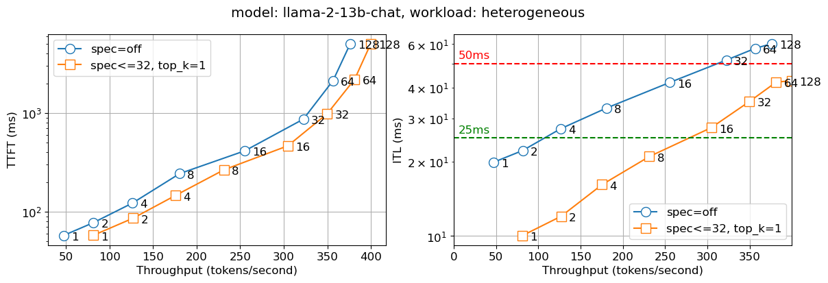
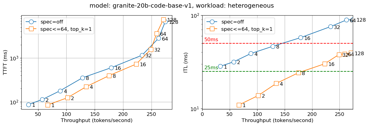
We deployed the above solution in an internal production environment. The figure below reports two metrics – time to first token (TTFT) and inter-token latency (ITL) with different numbers of concurrent users (which is captured in the numbers on the graph lines). We observe that the speculative decoding version is nearly twice as fast for the Llama2 13B chat model and nearly thrice as fast for the Granite 20B code model compared to the non-speculative version for all batch sizes. We observe similar behavior for the smaller models – IBM’s Granite 7B and Meta Llama3 8B models.

Time to first token (TTFT - left) and Inter-token latency (ITL - right) for Llama 13B with number of concurrent users indicated on the graph

Figure 3: Time to first token (TTFT – left) and Inter-token latency (ITL – right) for Llama 13B with number of concurrent users indicated on the graph

Time to first token (TTFT - left) and Inter-token latency (ITL - right) for Granite 20B Code with number of concurrent users indicated on the graph

Figure 4: Time to first token (TTFT – left) and Inter-token latency (ITL – right) for Granite 20B Code with number of concurrent users indicated on the graph

Note on efficiency

We performed numerous experiments to determine the right configuration for speculator training. These are:

  1. Speculator architecture: The current approach allows for the number of heads to be modified, which maps to the number of tokens that we can look ahead. Increasing the number of heads also increases the amount of extra compute needed and complexity of training. In practice, for language models, we find 3-4 heads works well in practice, whereas we found that code models can reap benefits from 6-8 heads.
  2. Compute: Increasing the number of heads results in increased compute in two dimensions, one is that of increased latency for a single forward pass as well as the compute needed for multiple tokens. If the speculator is not accurate with more heads, it will result in wasted compute increasing the latency and reducing the throughput.
  3. Memory: The increased compute is offset by the roundtrips to HBM that need to be done for each forward pass. Note that if we get 3 tokens lookahead correct, we have saved three round trip times on HBM.

We settled on 3-4 heads for the language models and 6-8 heads for the code models and across different model sizes ranging from 7B to 20B, we observed significant latency improvements without throughput loss compared to non-speculative decoding. We begin to observe throughput reduction beyond a batch size of 64, which happens rarely in practice.

Speculative decoding: Training

There are two broad approaches for speculative decoding, one is to leverage a smaller model (e.g., Llama 7B as a speculator for Llama 70B) and the other is to attach speculator heads (and train them). In our experiments, we find the approach of attaching speculator heads to be more effective both in model quality and latency gains.

Speculator architecture

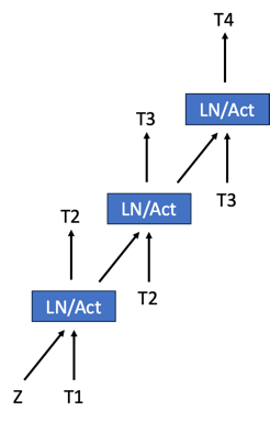
Medusa made speculative decoding popular; their approach is to add a head to the existing model which is then trained to do speculation. We modify the Medusa architecture by making the “heads” hierarchical, where each head stage predicts a single token and then feeds it to the next head stage. These multi-stage heads are depicted in the below figure. We are exploring ways of minimizing the embeddings table by sharing these across the multiple stages and base model.

A simple architecture diagram for a 3-headed multi-stage  speculator. Z is the state from the base model.

Figure 4: A simple architecture diagram for a 3-headed multi-stage speculator. Z is the state from the base model.

Speculator training

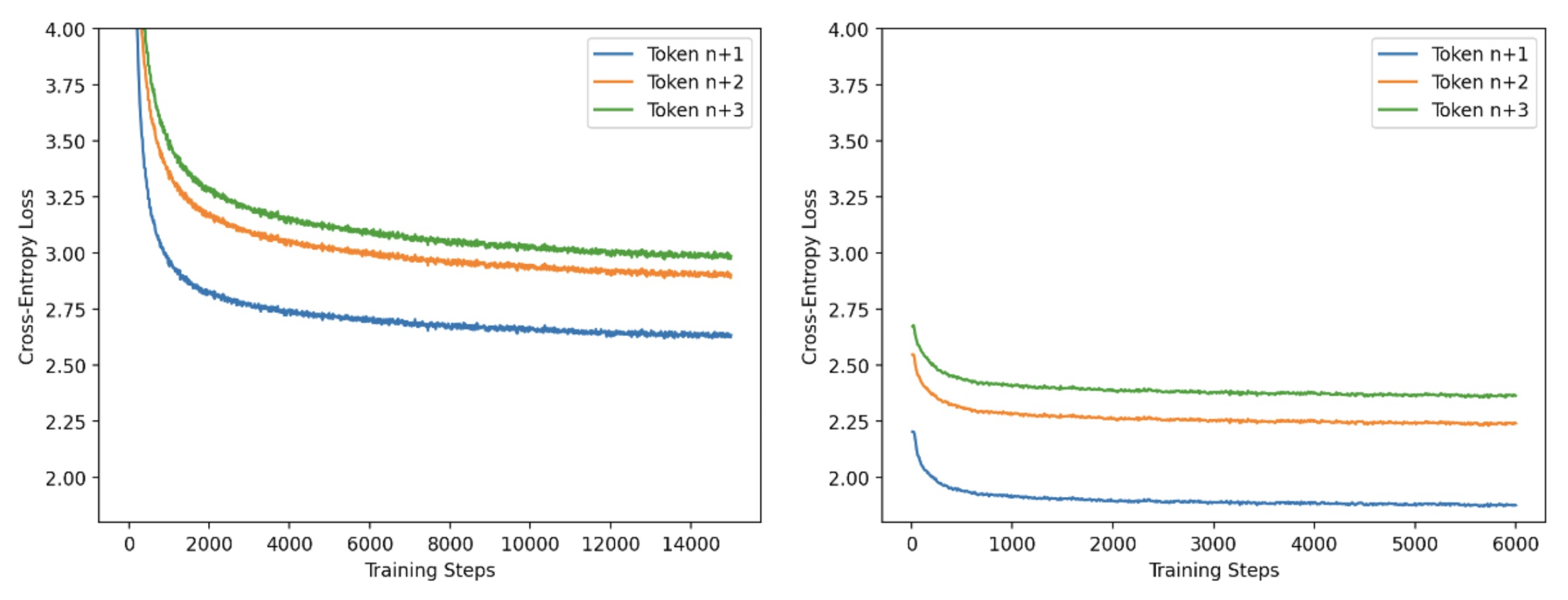
We have a two-phase approach to training a speculator for efficiency reasons. In the first phase, we train on small batches with long sequence lengths (4k tokens) and use the standard causal LM approach for training. In phase 2, we use large batches with short sequence lengths (256 tokens) generated from the base model. In this training phase, we tune the heads to match the output of the base model. Through numerous experiments, we find that a 5:2 ratio of steps for phase 1 vs phase 2 works well. We depict the progress of these phases in the below figure. We use PyTorch FSDP and IBM FMS for the training of speculators.

Per-head training loss curves for Llama2-13B speculator training, phase 1 and 2

Figure 5: Per-head training loss curves for Llama2-13B speculator training, phase 1 and 2

Conclusion and Future Work

Through this blog, we are releasing a new approach for speculative decoding and the following assets:

  1. Models for improving the inter-token latencies for a range of models – Llama3 8B, Llama2 13B, Granite 7B, and CodeLlama 13B
  2. Production quality code for inference
  3. Recipes for training speculators

We are working on training speculators for Llama3 70B and Mistral models and invite the community to contribute as well as help improve on our framework. We would also love to work with major open source serving frameworks such as vLLM and TGI to contribute back our speculative decoding approach to benefit the community.

Acknowledgements

There are several teams that helped us get to these latency improvements for inference. We would like to thank the vLLM team for creating the paged attention kernel in a clean and reusable manner. We extend our gratitude to the Team PyTorch at Meta that helped provide feedback on this blog as well as continued efforts on optimal usage of PyTorch. Special thanks to our internal production teams at IBM Research who took this prototype to production and hardened it. A shout out to Stas Bekman for providing insightful comments on the blog resulting in an improved explanation of the tradeoffs between compute, memory, and speculator effectiveness.

The paged attention kernel was integrated into IBM FMS by Josh Rosenkranz and Antoni Viros i Martin. The speculator architecture and training was done by Davis Wertheimer, Pavithra Ranganathan, and Sahil Suneja. The integration of the modeling code with the inference server was done by Thomas Parnell, Nick Hill, and Prashant Gupta.

Read More

Guiding Instruction-based Image Editing via Multimodal Large Language Models

Instruction-based image editing improves the controllability and flexibility of image manipulation via natural commands without elaborate descriptions or regional masks. However, human instructions are sometimes too brief for current methods to capture and follow. Multimodal large language models (MLLMs) show promising capabilities in cross-modal understanding and visual-aware response generation via LMs. We investigate how MLLMs facilitate edit instructions and present MLLM-Guided Image Editing (MGIE). MGIE learns to derive expressive instructions and provides explicit guidance. The editing…Apple Machine Learning Research

ReLU Strikes Back: Exploiting Activation Sparsity in Large Language Models

Large Language Models (LLMs) with billions of parameters have drastically transformed AI applications. However, their demanding computation during inference has raised significant challenges for deployment on resource-constrained devices. Despite recent trends favoring alternative activation functions such as GELU or SiLU, known for increased computation, this study strongly advocates for reinstating ReLU activation in LLMs. We demonstrate that using the ReLU activation function has a negligible impact on convergence and performance while significantly reducing computation and weight transfer…Apple Machine Learning Research

Pseudo-Generalized Dynamic View Synthesis from a Video

Rendering scenes observed in a monocular video from novel viewpoints is a chal- lenging problem. For static scenes the community has studied both scene-specific optimization techniques, which optimize on every test scene, and generalized tech- niques, which only run a deep net forward pass on a test scene. In contrast, for dy- namic scenes, scene-specific optimization techniques exist, but, to our best knowl- edge, there is currently no generalized method for dynamic novel view synthesis from a given monocular video. To explore whether generalized dynamic novel view synthesis from monocular…Apple Machine Learning Research