An Open Source Vibrotactile Haptics Platform for On-Body Applications

Posted by Artem Dementyev, Hardware Engineer, Google Research

Most wearable smart devices and mobile phones have the means to communicate with the user through tactile feedback, enabling applications from simple notifications to sensory substitution for accessibility. Typically, they accomplish this using vibrotactile actuators, which are small electric vibration motors. However, designing a haptic system that is well-targeted and effective for a given task requires experimentation with the number of actuators and their locations in the device, yet most practical applications require standalone on-body devices and integration into small form factors. This combination of factors can be difficult to address outside of a laboratory as integrating these systems can be quite time-consuming and often requires a high level of expertise.

A typical lab setup on the left and the VHP board on the right.

In “VHP: Vibrotactile Haptics Platform for On-body Applications”, presented at ACM UIST 2021, we develop a low-power miniature electronics board that can drive up to 12 independent channels of haptic signals with arbitrary waveforms. The VHP electronics board can be battery-powered, and integrated into wearable devices and small gadgets. It allows all-day wear, has low latency, battery life between 3 and 25 hours, and can run 12 actuators simultaneously. We show that VHP can be used in bracelet, sleeve, and phone-case form factors. The bracelet was programmed with an audio-to-tactile interface to aid lipreading and remained functional when worn for multiple months by developers. To facilitate greater progress in the field of wearable multi-channel haptics with the necessary tools for their design, implementation, and experimentation, we are releasing the hardware design and software for the VHP system via GitHub.

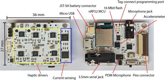
Front and back sides of the VHP circuit board.
Block diagram of the system.

Platform Specifications.
VHP consists of a custom designed circuit board, where the main components are the microcontroller and haptic amplifier, which converts microcontroller’s digital output into signals that drive the actuators. The haptic actuators can be controlled by signals arriving via serial, USB, and Bluetooth Low Energy (BLE), as well as onboard microphones, using an nRF52840 microcontroller, which was chosen because it offers many input and output options and BLE, all in a small package. We added several sensors into the board to provide more experimental flexibility: an on-board digital microphone, an analog microphone amplifier, and an accelerometer. The firmware is a portable C/C++ library that works in the Arduino ecosystem.

To allow for rapid iteration during development, the interface between the board and actuators is critical. The 12 tactile signals’ wiring have to be quick to set up in order to allow for such development, while being flexible and robust to stand up to prolonged use. For the interface, we use a 24-pin FPC (flexible printed circuit) connector on the VHP. We support interfacing to the actuators in two ways: with a custom flexible circuit board and with a rigid breakout board.

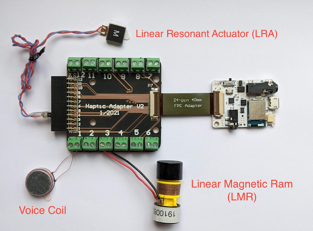
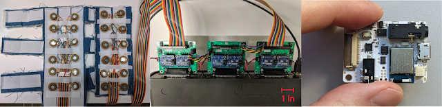
VHP board (small board on the right) connected to three different types of tactile actuators via rigid breakout board (large board on the left).

Using Haptic Actuators as Sensors
In our previous blog post, we explored how back-EMF in a haptic actuator could be used for sensing and demonstrated a variety of useful applications. Instead of using back-EMF sensing in the VHP system, we measure the electrical current that drives each vibrotactile actuator and use the current load as the sensing mechanism. Unlike back-EMF sensing, this current-sensing approach allows simultaneous sensing and actuation, while minimizing the additional space needed on the board.

One challenge with the current-sensing approach is that there is a wide variety of vibrotactile actuators, each of which may behave differently and need different presets. In addition, because different actuators can be added and removed during prototyping with the adapter board, it would be useful if the VHP were able to identify the actuator automatically. This would improve the speed of prototyping and make the system more novice-friendly.

To explore this possibility, we collected current-load data from three off-the-shelf haptic actuators and trained a simple support vector machine classifier to recognize the difference in the signal pattern between actuators. The test accuracy was 100% for classifying the three actuators, indicating that each actuator has a very distinct response.

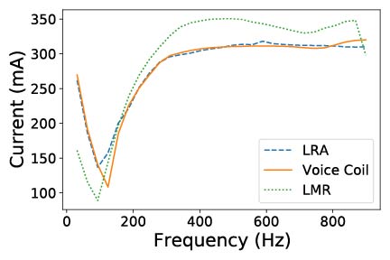
Different actuators have a different current signature during a frequency sweep, thus allowing for automatic identification.

Additionally, vibrotactile actuators require proper contact with the skin for consistent control over stimulation. Thus, the device should measure skin contact and either provide an alert or self-adjust if it is not loaded correctly. To test whether a skin contact measuring technique works in practice, we measured the current load on actuators in a bracelet as it was tightened and loosened around the wrist. As the bracelet strap is tightened, the contact pressure between the skin and the actuator increases and the current required to drive the actuator signal increases commensurately.

Current load sensing is responding to touch, while the actuator is driven at 250 Hz frequency.

Quality of the fit of the bracelet is measured.

Audio-to-Tactile Feedback
To demonstrate the utility of the VHP platform, we used it to develop an audio-to-tactile feedback device to help with lipreading. Lipreading can be difficult for many speech sounds that look similar (visemes), such as “pin” and “min”. In order to help the user differentiate visemes like these, we attach a microphone to the VHP system, which can then pick up the speech sounds and translate the audio to vibrations on the wrist. For audio-to-tactile translation, we used our previously developed algorithms for real-time audio-to-tactile conversion, available via GitHub. Briefly, audio filters are paired with neural networks to recognize certain viesemes (e.g., picking up the hard consonant “p” in “pin”), and are then translated to vibrations in different parts of the bracelet. Our approach is inspired by tactile phonemic sleeve (TAPS), however the major difference is that in our approach the tactile signal is presented continuously and in real-time.

One of the developers who employs lipreading in daily life wore the bracelet daily for several months and found it to give better information to facilitate lipreading than previous devices, allowing improved understanding of lipreading visemes with the bracelet versus lipreading alone. In the future, we plan to conduct full-scale experiments with multiple users wearing the device for an extended time.

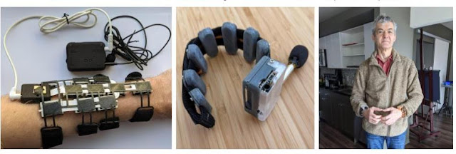
Left: Audio-to-tactile sleeve. Middle: Audio-to-tactile bracelet. Right: One of our developers tests out the bracelets, which are worn on both arms.

Potential Applications
The VHP platform enables rapid experimentation and prototyping that can be used to develop techniques for a variety of applications. For example:

  • Rich haptics on small devices: Expanding the number of actuators on mobile phones, which typically only have one or two, could be useful to provide additional tactile information. This is especially useful as fingers are sensitive to vibrations. We demonstrated a prototype mobile phone case with eight vibrotactile actuators. This could be used to provide rich notifications and enhance effects in a mobile game or when watching a video.
  • Lab psychophysical experiments: Because VHP can be easily set up to send and receive haptic signals in real time, e.g., from a Jupyter notebook, it could be used to perform real-time haptic experiments.
  • Notifications and alerts: The wearable VHP could be used to provide haptic notifications from other devices, e.g., alerting if someone is at the door, and could even communicate distinguishable alerts through use of multiple actuators.
  • Sensory substitution: Besides the lipreading assistance example above, there are many other potential applications for accessibility using sensory substitution, such as visual-to-tactile sensing or even sensing magnetic fields.
  • Loading sensing: The ability to sense from the haptic actuator current load is unique to our platform, and enables a variety of features, such as pressure sensing or automatically adjusting actuator output.
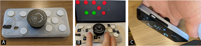
Integrating eight voice coils into a phone case. We used loading sensing to understand which voice coils are being touched.

What’s next?
We hope that others can utilize the platform to build a diverse set of applications. If you are interested and have ideas about using our platform or want to receive updates, please fill out this form. We hope that with this platform, we can help democratize the use of haptics and inspire a more widespread use of tactile devices.

Acknowledgments
This work was done by Artem Dementyev, Pascal Getreuer, Dimitri Kanevsky, Malcolm Slaney and Richard Lyon. We thank Alex Olwal, Thad Starner, Hong Tan, Charlotte Reed, Sarah Sterman for valuable feedback and discussion on the paper. Yuhui Zhao, Dmitrii Votintcev, Chet Gnegy, Whitney Bai and Sagar Savla for feedback on the design and engineering.

Read More

Dexterous robotic hands manipulate thousands of objects with ease

At just one year old, a baby is more dexterous than a robot. Sure, machines can do more than just pick up and put down objects, but we’re not quite there as far as replicating a natural pull toward exploratory or sophisticated dexterous manipulation goes. 

Artificial intelligence firm OpenAI gave it a try with Dactyl (meaning “finger,” from the Greek word “daktylos”), using their humanoid robot hand to solve a Rubik’s cube with software that’s a step toward more general AI, and a step away from the common single-task mentality. DeepMind created “RGB-Stacking,” a vision-based system that challenges a robot to learn how to grab items and stack them. 

Scientists from MIT’s Computer Science and Artificial Intelligence Laboratory (CSAIL), in the ever-present quest to get machines to replicate human abilities, created a framework that’s more scaled up: a system that can reorient over 2,000 different objects, with the robotic hand facing both upwards and downwards. This ability to manipulate anything from a cup to a tuna can to a Cheez-It box could help the hand quickly pick-and-place objects in specific ways and locations — and even generalize to unseen objects. 

This deft “handiwork” — which is usually limited to single tasks and upright positions — could be an asset in speeding up logistics and manufacturing, helping with common demands such as packing objects into slots for kitting, or dexterously manipulating a wider range of tools. The team used a simulated, anthropomorphic hand with 24 degrees of freedom, and showed evidence that the system could be transferred to a real robotic system in the future. 

“In industry, a parallel-jaw gripper is most commonly used, partially due to its simplicity in control, but it’s physically unable to handle many tools we see in daily life,” says MIT CSAIL PhD student Tao Chen, member of the MIT Improbable AI Lab and the lead researcher on the project. “Even using a plier is difficult because it can’t dexterously move one handle back and forth. Our system will allow a multi-fingered hand to dexterously manipulate such tools, which opens up a new area for robotics applications.”

This type of “in-hand” object reorientation has been a challenging problem in robotics, due to the large number of motors to be controlled and the frequent change in contact state between the fingers and the objects. And with over 2,000 objects, the model had a lot to learn. 

The problem becomes even more tricky when the hand is facing downwards. Not only does the robot need to manipulate the object, but also circumvent gravity so it doesn’t fall down. 

The team found that a simple approach could solve complex problems. They used a model-free reinforcement learning algorithm (meaning the system has to figure out value functions from interactions with the environment) with deep learning, and something called a “teacher-student” training method. 

For this to work, the “teacher” network is trained on information about the object and robot that’s easily available in simulation, but not in the real world, such as the location of fingertips or object velocity. To ensure that the robots can work outside of the simulation, the knowledge of the “teacher” is distilled into observations that can be acquired in the real world, such as depth images captured by cameras, object pose, and the robot’s joint positions. They also used a “gravity curriculum,” where the robot first learns the skill in a zero-gravity environment, and then slowly adapts the controller to the normal gravity condition, which, when taking things at this pace, really improved the overall performance. 

While seemingly counterintuitive, a single controller (known as brain of the robot) could reorient a large number of objects it had never seen before, and with no knowledge of shape. 

“We initially thought that visual perception algorithms for inferring shape while the robot manipulates the object was going to be the primary challenge,” says MIT Professor Pulkit Agrawal, an author on the paper about the research. “To the contrary, our results show that one can learn robust control strategies that are shape-agnostic. This suggests that visual perception may be far less important for manipulation than what we are used to thinking, and simpler perceptual processing strategies might suffice.” 

Many small, circular shaped objects (apples, tennis balls, marbles), had close to 100 percent success rates when reoriented with the hand facing up and down, with the lowest success rates, unsurprisingly, for more complex objects, like a spoon, a screwdriver, or scissors, being closer to 30 percent. 

Beyond bringing the system out into the wild, since success rates varied with object shape, in the future, the team notes that training the model based on object shapes could improve performance. 

Chen wrote a paper about the research alongside MIT CSAIL PhD student Jie Xu and MIT Professor Pulkit Agrawal. The research is funded by Toyota Research Institute, Amazon Research Award, and DARPA Machine Common Sense Program. It will be presented at the 2021 The Conference on Robot Learning (CoRL).

Read More

Making Better Future Predictions by Watching Unlabeled Videos

Posted by Dave Epstein, Student Researcher and Chen Sun, Staff Research Scientist, Google Research

Machine learning (ML) agents are increasingly deployed in the real world to make decisions and assist people in their daily lives. Making reasonable predictions about the future at varying timescales is one of the most important capabilities for such agents because it enables them to predict changes in the world around them, including other agents’ behaviors, and plan how to act next. Importantly, successful future prediction requires both capturing meaningful transitions in the environment (e.g., dough transforming into bread) and adapting to how transitions unfold over time in order to make decisions.

Previous work in future prediction from visual observations has largely been constrained by the format of its output (e.g., pixels that represent an image) or a manually-defined set of human activities (e.g., predicting if someone will keep walking, sit down, or jump). These are either too detailed and hard to predict or lack important information about the richness of the real world. For example, predicting “person jumping” does not capture why they’re jumping, what they’re jumping onto, etc. Also, with very few exceptions, previous models were designed to make predictions at a fixed offset into the future, which is a limiting assumption because we rarely know when meaningful future states will happen.

For example, in a video about making ice cream (depicted below), the meaningful transition from “cream” to “ice cream” occurs over 35 seconds, so models predicting such transitions would need to look 35 seconds ahead. But this time interval varies a large amount across different activities and videos — meaningful transitions occur at any distance into the future. Learning to make such predictions at flexible intervals is hard because the desired ground truth may be relatively ambiguous. For example, the correct prediction could be the just-churned ice cream in the machine, or scoops of the ice cream in a bowl. In addition, collecting such annotations at scale (i.e., frame-by-frame for millions of videos) is infeasible. However, many existing instructional videos come with speech transcripts, which often offer concise, general descriptions throughout entire videos. This source of data can guide a model’s attention toward important parts of the video, obviating the need for manual labeling and allowing a flexible, data-driven definition of the future.

In “Learning Temporal Dynamics from Cycles in Narrated Video”, published at ICCV 2021, we propose an approach that is self-supervised, using a recent large unlabeled dataset of diverse human action. The resulting model operates at a high level of abstraction, can make predictions arbitrarily far into the future, and chooses how far into the future to predict based on context. Called Multi-Modal Cycle Consistency (MMCC), it leverages narrated instructional video to learn a strong predictive model of the future. We demonstrate how MMCC can be applied, without fine-tuning, to a variety of challenging tasks, and qualitatively examine its predictions. In the example below, MMCC predicts the future (d) from present frame (a), rather than less relevant potential futures (b) or (c).

This work uses cues from vision and language to predict high-level changes (such as cream becoming ice cream) in video (video from HowTo100M).

Viewing Videos as Graphs
The foundation of our method is to represent narrated videos as graphs. We view videos as a collection of nodes, where nodes are either video frames (sampled at 1 frame per second) or segments of narrated text (extracted with automatic speech recognition systems), encoded by neural networks. During training, MMCC constructs a graph from the nodes, using cross-modal edges to connect video frames and text segments that refer to the same state, and temporal edges to connect the present (e.g., strawberry-flavored cream) and the future (e.g., soft-serve ice cream). The temporal edges operate on both modalities equally — they can start from either a video frame, some text, or both, and can connect to a future (or past) state in either modality. MMCC achieves this by learning a latent representation shared by frames and text and then making predictions in this representation space.

Multi-modal Cycle Consistency
To learn the cross-modal and temporal edge functions without supervision, we apply the idea of cycle consistency. Here, cycle consistency refers to the construction of cycle graphs, in which the model constructs a series of edges from an initial node to other nodes and back again: Given a start node (e.g., a sample video frame), the model is expected to find its cross-modal counterpart (i.e., text describing the frame) and combine them as the present state. To do this, at the start of training, the model assumes that frames and text with the same timestamps are counterparts, but then relaxes this assumption later. The model then predicts a future state, and the node most similar to this prediction is selected. Finally, the model attempts to invert the above steps by predicting the present state backward from the future node, and thus connecting the future node back with the start node.

The discrepancy between the model’s prediction of the present from the future and the actual present is the cycle-consistency loss. Intuitively, this training objective requires the predicted future to contain enough information about its past to be invertible, leading to predictions that correspond to meaningful changes to the same entities (e.g., tomato becoming marinara sauce, or flour and eggs in a bowl becoming dough). Moreover, the inclusion of cross-modal edges ensures future predictions are meaningful in either modality.

To learn the temporal and cross-modal edge functions end-to-end, we use the soft attention technique, which first outputs how likely each node is to be the target node of the edge, and then “picks” a node by taking the weighted average among all possible candidates. Importantly, this cyclic graph constraint makes few assumptions for the kind of temporal edges the model should learn, as long as they end up forming a consistent cycle. This enables the emergence of long-term temporal dynamics critical for future prediction without requiring manual labels of meaningful changes.

An example of the training objective: A cycle graph is expected to be constructed between the chicken with soy sauce and the chicken in chili oil because they are two adjacent steps in the chicken’s preparation (video from HowTo100M).

Discovering Cycles in Real-World Video
MMCC is trained without any explicit ground truth, using only long video sequences and randomly sampled starting conditions (a frame or text excerpt) and asking the model to find temporal cycles. After training, MMCC can identify meaningful cycles that capture complex changes in video.

Given frames as input (left), MMCC selects relevant text from video narrations and uses both modalities to predict a future frame (middle). It then finds text relevant to this future and uses it to predict the past (right). Using its knowledge of how objects and scenes change over time, MMCC “closes the cycle” and ends up where it started (videos from HowTo100M).
The model can also start from narrated text rather than frames and still find relevant transitions (videos from HowTo100M).

Zero-Shot Applications
For MMCC to identify meaningful transitions over time in an entire video, we define a “likely transition score” for each pair (A, B) of frames in a video, according to the model’s predictions — the closer B is to our model’s prediction of the future of A, the higher the score assigned. We then rank all pairs according to this score and show the highest-scoring pairs of present and future frames detected in previously unseen videos (examples below).

The highest-scoring pairs from eight random videos, which showcase the versatility of the model across a wide range of tasks (videos from HowTo100M).

We can use this same approach to temporally sort an unordered collection of video frames without any fine-tuning by finding an ordering that maximizes the overall confidence scores between all adjacent frames in the sorted sequence.

Left: Shuffled frames from three videos. Right: MMCC unshuffles the frames. The true order is shown under each frame. Even when MMCC does not predict the ground truth, its predictions often appear reasonable, and so, it can present an alternate ordering (videos from HowTo100M).

Evaluating Future Prediction
We evaluate the model’s ability to anticipate action, potentially minutes in advance, using the top-k recall metric, which here measures a model’s ability to retrieve the correct future (higher is better). On CrossTask, a dataset of instruction videos with labels describing key steps, MMCC outperforms the previous self-supervised state-of-the-art models in inferring possible future actions.

Recall
Model    Top-1       Top-5       Top-10   
Cross-modal    2.9 14.2 24.3
Repr. Ant. 3.0 13.3 26.0
MemDPC 2.9 15.8 27.4
TAP 4.5 17.1 27.9
MMCC 5.4 19.9 33.8

Conclusions
We have introduced a self-supervised method to learn temporal dynamics by cycling through narrated instructional videos. Despite the simplicity of the model’s architecture, it can discover meaningful long-term transitions in vision and language, and can be applied without further training to challenging downstream tasks, such as anticipating far-away action and ordering collections of images. An interesting future direction is transferring the model to agents so they can use it to conduct long-term planning.

Acknowledgements
The core team includes Dave Epstein, Jiajun Wu, Cordelia Schmid, and Chen Sun. We thank Alexei Efros, Mia Chiquier, and Shiry Ginosar for their feedback, and Allan Jabri for inspiration in figure design. Dave would like to thank Dídac Surís and Carl Vondrick for insightful early discussions on cycling through time in video.

Read More

Women in Machine Learning Symposium – Event Recap

Posted by Joana Carrasqueira, Program Manager, TensorFlow.

Thank you to everyone who joined us at the first Women in Machine Learning Symposium!

Hundreds of practitioners joined from all over the world to share tips and insights for careers in ML, how to be involved in the community, contribute to open source, and much more. It was very inspiring to learn from each other’s experiences. Following is a quick recap, and an overview of the resources we discussed at the event. Thanks again.

Online education

Get involved in the community

Build your portfolio

Connect with (or become) a GDE

Read More

What’s new in TensorFlow 2.7?

Posted by Goldie Gadde and Josh Gordon for the TensorFlow team

TensorFlow 2.7 is here! This release improves usability with clearer error messages, simplified stack traces, and adds new tools and documentation for users migrating to TF2.

Improved Debugging Experience

The process of debugging your code is a fundamental part of the user experience of a machine learning framework. In this release, we’ve considerably improved the TensorFlow debugging experience to make it more productive and more enjoyable, via three major changes: simplified stack traces, displaying additional context information in errors that originate from custom Keras layers, and a wide-ranging audit of all error messages in Keras and TensorFlow.

Simplified stack traces

TensorFlow is now filtering by default the stack traces displayed upon error to hide any frame that originates from TensorFlow-internal code, and keep the information focused on what matters to you: your own code. This makes stack traces simpler and shorter, and it makes it easier to understand and fix the problems in your code.

If you’re actually debugging the TensorFlow codebase itself (for instance, because you’re preparing a PR for TensorFlow), you can turn off the filtering mechanism by calling tf.debugging.disable_traceback_filtering().

Automatic context injection for Keras layer exceptions

One of the most common use cases for writing low-level code is creating custom Keras layers, so we wanted to make debugging your layers as easy and productive as possible. The first thing you do when you’re debugging a layer is to print the shapes and dtypes of its inputs, as well the value of its training and mask arguments. We now add this information automatically to all stack traces that originate from custom Keras layers.

See the effect of stack trace filtering and call context information display in practice in the image below:

Simplified stack traces in TensorFlow 2.7

Audit and improve all error messages in the TensorFlow and Keras codebases

Lastly, we’ve audited every error message in the Keras and TensorFlow codebases (thousands of error locations!) and improved them to make sure they follow UX best practices. A good error message should tell you what the framework expected, what you did that didn’t match the framework’s expectations, and should provide tips to fix the problem.

Improve tf.function error messages

We have improved two common types of tf.function error messages: runtime error messages and “Graph” tensor error messages, by including tracebacks pointing to the error source in the user code. For other vague and inaccurate tf.function error messages, we also updated them to be more clear and accurate.

For the runtime error message caused by the user code

@tf.function
def f():
l = tf.range(tf.random.uniform((), minval=1, maxval=10, dtype=tf.int32))
return l[20]

A summary of the old error message looks like

# … Python stack trace of the function call …

InvalidArgumentError: slice index 20 of dimension 0 out of bounds.
[[node strided_slice (defined at <'ipython-input-8-250c76a76c0e'>:5) ]] [Op:__inference_f_75]

Errors may have originated from an input operation.
Input Source operations connected to node strided_slice:
range (defined at <ipython-input-8-250c76a76c0e >':4)

Function call stack:
f

A summary of the new error message looks like

# … Python stack trace of the function call …

InvalidArgumentError: slice index 20 of dimension 0 out of bounds.
[[node strided_slice
(defined at <ipython-input-3-250c76a76c0e>:5)
]] [Op:__inference_f_15]

Errors may have originated from an input operation.
Input Source operations connected to node strided_slice:
In[0] range (defined at <ipython-input-3-250c76a76c0e>:4)
In[1] strided_slice/stack:
In[2] strided_slice/stack_1:
In[3] strided_slice/stack_2:

Operation defined at: (most recent call last)
# … Stack trace of the error within the function …
>>> File "<ipython-input-3-250c76a76c0e>", line 7, in <module>
>>> f()
>>>
>>> File "<ipython-input-3-250c76a76c0e>", line 5, in f
>>> return l[20]
>>>

The main difference is runtime errors raised while executing a tf.function now include a stack trace which shows the source of the error, in the user’s code.

# … Original error message and information …
# … More stack frames …
>>> File "<ipython-input-3-250c76a76c0e>", line 7, in <module>
>>> f()
>>>
>>> File "<ipython-input-3-250c76a76c0e>", line 5, in f
>>> return l[20]
>>>

For the “Graph” tensor error messages caused by the following user code

x = None

@tf.function
def leaky_function(a):
global x
x = a + 1 # Bad - leaks local tensor
return a + 2

@tf.function
def captures_leaked_tensor(b):
b += x
return b

leaky_function(tf.constant(1))
captures_leaked_tensor(tf.constant(2))

A summary of the old error message looks like

# … Python stack trace of the function call …

TypeError: An op outside of the function building code is being passed
a "Graph" tensor. It is possible to have Graph tensors
leak out of the function building context by including a
tf.init_scope in your function building code.
For example, the following function will fail:
@tf.function
def has_init_scope():
my_constant = tf.constant(1.)
with tf.init_scope():
added = my_constant * 2
The graph tensor has name: add:0

A summary of the new error message looks like

# … Python stack trace of the function call …

TypeError: Originated from a graph execution error.

The graph execution error is detected at a node built at (most recent call last):
# … Stack trace of the error within the function …
>>> File <ipython-input-5-95ca3a98778f>, line 6, in leaky_function
# … More stack trace of the error within the function …

Error detected in node 'add' defined at: File "<ipython-input-5-95ca3a98778f>", line 6, in leaky_function

TypeError: tf.Graph captured an external symbolic tensor. The symbolic tensor 'add:0' created by node 'add' is captured by the tf.Graph being executed as an input. But a tf.Graph is not allowed to take symbolic tensors from another graph as its inputs. Make sure all captured inputs of the executing tf.Graph are not symbolic tensors. Use return values, explicit Python locals or TensorFlow collections to access it. Please see https://www.tensorflow.org/guide/function#all_outputs_of_a_tffunction_must_be_return_values for more information.

The main difference is errors for attempting to capture a tensor that was leaked from an unreachable graph now include a stack trace which shows where the tensor was created in the user’s code:

# … Original error message and information …
# … More stack frames …
>>> File <ipython-input-5-95ca3a98778f>, line 6, in leaky_function

Error detected in node 'add' defined at: File "<ipython-input-5-95ca3a98778f>", line 6, in leaky_function

TypeError: tf.Graph captured an external symbolic tensor. The symbolic tensor 'add:0' created by node 'add' is captured by the tf.Graph being executed as an input. But a tf.Graph is not allowed to take symbolic tensors from another graph as its inputs. Make sure all captured inputs of the executing tf.Graph are not symbolic tensors. Use return values, explicit Python locals or TensorFlow collections to access it. Please see https://www.tensorflow.org/guide/function#all_outputs_of_a_tffunction_must_be_return_values for more information.

Introducing tf.experimental.ExtensionType

User-defined types can make your projects more readable, modular, maintainable. TensorFlow 2.7.0 introduces the ExtensionType API, which can be used to create user-defined object-oriented types that work seamlessly with TensorFlow’s APIs. Extension types are a great way to track and organize the tensors used by complex models. Extension types can also be used to define new tensor-like types, which specialize or extend the basic concept of “Tensor.” To create an extension type, simply define a Python class with tf.experimental.ExtensionType as its base, and use type annotations to specify the type for each field:

class TensorGraph(tf.experimental.ExtensionType):
"""A collection of labeled nodes connected by weighted edges."""
edge_weights: tf.Tensor # shape=[num_nodes, num_nodes]
node_labels: typing.Mapping[str, tf.Tensor] # shape=[num_nodes]; dtype=any

class MaskedTensor(tf.experimental.ExtensionType):
"""A tensor paired with a boolean mask, indicating which values are valid."""
values: tf.Tensor
mask: tf.Tensor # shape=values.shape; false for missing/invalid values.

class CSRSparseMatrix(tf.experimental.ExtensionType):
"""Compressed sparse row matrix (https://en.wikipedia.org/wiki/Sparse_matrix)."""
values: tf.Tensor # shape=[num_nonzero]; dtype=any
col_index: tf.Tensor # shape=[num_nonzero]; dtype=int64
row_index: tf.Tensor # shape=[num_rows+1]; dtype=int64

The ExtensionType base class adds a constructor and special methods based on the field type annotations (similar to typing.NamedTuple and @dataclasses.dataclass from the standard Python library). You can optionally customize the type by overriding these defaults, or adding new methods, properties, or subclasses.

Extension types are supported by the following TensorFlow APIs:

  • Keras: Extension types can be used as inputs and outputs for Keras Models and Layers.
  • Dataset: Extension types can be included in Datasets, and returned by dataset Iterators.
  • TensorFlow hub: Extension types can be used as inputs and outputs for tf.hub modules.
  • SavedModel: Extension types can be used as inputs and outputs for SavedModel functions.
  • tf.function: Extension types can be used as arguments and return values for functions wrapped with the @tf.function decorator.
  • control flow: Extension types can be used by control flow operations, such as tf.cond and tf.while_loop. This includes control flow operations added by autograph.
  • tf.py_function: Extension types can be used as arguments and return values for the func argument to tf.py_function.
  • Tensor ops: Extension types can be extended to support most TensorFlow ops that accept Tensor inputs (e.g., tf.matmul, tf.gather, and tf.reduce_sum), using dispatch decorators.
  • distribution strategy: Extension types can be used as per-replica values.

For more information about extension types, see the Extension Type guide.

Note: The tf.experimental prefix indicates that this is a new API, and we would like to collect feedback from real-world usage; barring any unforeseen design issues, we plan to migrate ExtensionType out of the experimental package in accordance with the TF experimental policy.

TF2 Migration made easier!

To support users interested in migrating their workloads from TF1 to TF2, we have created a new Migrate to TF2 tab on the TensorFlow website, which includes updated guides and completely new documentation with concrete, runnable examples in Colab.

A new shim tool has been added which dramatically eases migration of variable_scope-based models to TF2. It is expected to enable most TF1 users to run existing model architectures as-is (or with only minor adjustments) in TF2 pipelines without having to rewrite your modeling code. You can learn more about it in the model mapping guide.

New community contributed models on TensorFlow Hub

Since the last TensorFlow release, the community really came together to make many new models available on TensorFlow Hub. Now you can find models like MLP-Mixer, Vision Transformers, Wav2Vec2, RoBERTa, ConvMixer, DistillBERT, YoloV5 and many more. All of these models are ready to use via TensorFlow Hub. You can learn more about publishing your models here.

Next steps

Check out the release notes for more information. To stay up to date, you can read the TensorFlow blog, follow twitter.com/tensorflow, or subscribe to youtube.com/tensorflow. If you’ve built something you’d like to share, please submit it for our Community Spotlight at goo.gle/TFCS. For feedback, please file an issue on GitHub or post to the TensorFlow Forum. Thank you!

Read More

Model Ensembles Are Faster Than You Think

Posted by Xiaofang Wang, Intern and Yair Alon (prev. Movshovitz-Attias), Software Engineer, Google Research

When building a deep model for a new machine learning application, researchers often begin with existing network architectures, such as ResNets or EfficientNets. If the initial model’s accuracy isn’t high enough, a larger model may be a tempting alternative, but may not actually be the best solution for the task at hand. Instead, better performance potentially could be achieved by designing a new model that is optimized for the task. However, such efforts can be challenging and usually require considerable resources.

In “Wisdom of Committees: An Overlooked Approach to Faster and More Accurate Models”, we discuss model ensembles and a subset called model cascades, both of which are simple approaches that construct new models by collecting existing models and combining their outputs. We demonstrate that ensembles of even a small number of models that are easily constructed can match or exceed the accuracy of state-of-the-art models while being considerably more efficient.

What Are Model Ensembles and Cascades?
Ensembles and cascades are related approaches that leverage the advantages of multiple models to achieve a better solution. Ensembles execute multiple models in parallel and then combine their outputs to make the final prediction. Cascades are a subset of ensembles, but execute the collected models sequentially, and merge the solutions once the prediction has a high enough confidence. For simple inputs, cascades use less computation, but for more complex inputs, may end up calling on a greater number of models, resulting in higher computation costs.

Overview of ensembles and cascades. While this example shows 2-model combinations for both ensembles and cascades, any number of models can potentially be used.

Compared to a single model, ensembles can provide improved accuracy if there is variety in the collected models’ predictions. For example, the majority of images in ImageNet are easy for contemporary image recognition models to classify, but there are many images for which predictions vary between models and that will benefit most from an ensemble.

While ensembles are well-known, they are often not considered a core building block of deep model architectures and are rarely explored when researchers are developing more efficient models (with a few notable exceptions [1, 2, 3]). Therefore, we conduct a comprehensive analysis of ensemble efficiency and show that a simple ensemble or cascade of off-the-shelf pre-trained models can enhance both the efficiency and accuracy of state-of-the-art models.

To encourage the adoption of model ensembles, we demonstrate the following beneficial properties:

  1. Simple to build: Ensembles do not require complicated techniques (e.g., early exit policy learning).
  2. Easy to maintain: Ensembles are trained independently, making them easy to maintain and deploy.
  3. Affordable to train: The total training cost of models in an ensemble is often lower than a similarly accurate single model.
  4. On-device speedup: The reduction in computation cost (FLOPS) successfully translates to a speedup on real hardware.

Efficiency and Training Speed
It’s not surprising that ensembles can increase accuracy, but using multiple models in an ensemble may introduce extra computational cost at runtime. So, we investigate whether an ensemble can be more accurate than a single model that has the same computational cost. We analyze a series of models, EfficientNet-B0 to EfficientNet-B7, that have different levels of accuracy and FLOPS when applied to ImageNet inputs. The ensemble predictions are computed by averaging the predictions of each individual model.

We find that ensembles are significantly more cost-effective in the large computation regime (>5B FLOPS). For example, an ensemble of two EfficientNet-B5 models matches the accuracy of a single EfficientNet-B7 model, but does so using ~50% fewer FLOPS. This demonstrates that instead of using a large model, in this situation, one should use an ensemble of multiple considerably smaller models, which will reduce computation requirements while maintaining accuracy. Moreover, we find that the training cost of an ensemble can be much lower (e.g., two B5 models: 96 TPU days total; one B7 model: 160 TPU days). In practice, model ensemble training can be parallelized using multiple accelerators leading to further reductions. This pattern holds for the ResNet and MobileNet families as well.

Ensembles outperform single models in the large computation regime (>5B FLOPS).

Power and Simplicity of Cascades
While we have demonstrated the utility of model ensembles, applying an ensemble is often wasteful for easy inputs where a subset of the ensemble will give the correct answer. In these situations, cascades save computation by allowing for an early exit, potentially stopping and outputting an answer before all models are used. The challenge is to determine when to exit from the cascade.

To highlight the practical benefit of cascades, we intentionally choose a simple heuristic to measure the confidence of the prediction — we take the confidence of the model to be the maximum of the probabilities assigned to each class. For example, if the predicted probabilities for an image being either a cat, dog, or horse were 20%, 80% and 20%, respectively, then the confidence of the model’s prediction (dog) would be 0.8. We use a threshold on the confidence score to determine when to exit from the cascade.

To test this approach, we build model cascades for the EfficientNet, ResNet, and MobileNetV2 families to match either computation costs or accuracy (limiting the cascade to a maximum of four models). By design in cascades, some inputs incur more FLOPS than others, because more challenging inputs go through more models in the cascade than easier inputs. So we report the average FLOPS computed over all test images. We show that cascades outperform single models in all computation regimes (when FLOPS range from 0.15B to 37B) and can enhance accuracy or reduce the FLOPS (sometimes both) for all models tested.

Cascades of EfficientNet (left), ResNet (middle) and MobileNetV2 (right) models on ImageNet. When using similar FLOPS, cascades obtain a higher accuracy than single models (shown by the red arrows pointing up). Cascades can also match the accuracy of single models with significantly fewer FLOPS e.g., 5.4x for B7 (green arrows pointing left).
Summary of accuracy vs. FLOPS for ensembles and cascades. Squares and stars represent ensembles and cascades, respectively,, and the “+” notation indicates the models that comprise the ensemble or cascade. For example, ”B3+B4+B5+B7” at a star refers to a cascade of EfficientNet-B3, B4, B5 and B7 models.

In some cases it is not the average computation cost but the worst-case cost that is the limiting factor. By adding a simple constraint to the cascade building procedure, one can guarantee an upper bound to the computation cost of the cascade. See the paper for more details.

Other than convolutional neural networks, we also consider a Transformer-based architecture, ViT. We build a cascade of ViT-Base and ViT-Large models to match the average computation or accuracy of a single state-of-the-art ViT-Large model, and show that the benefit of cascades also generalizes to Transformer-based architectures.

        Single Models Cascades – Similar Throughput    Cascades – Similar Accuracy
Top-1 (%) Throughput Top-1 (%) Throughput △Top-1 Top-1 (%) Throughput SpeedUp
ViT-L-224 82.0 192 83.1 221 1.1 82.3 409 2.1x
ViT-L-384 85.0 54 86.0 69 1.0 85.2 125 2.3x
Cascades of ViT models on ImageNet. “224” and “384” indicate the image resolution on which the model is trained. Throughput is measured as the number of images processed per second. Our cascades can achieve a 1.0% higher accuracy than ViT-L-384 with a similar throughput or achieve a 2.3x speedup over that model while matching its accuracy.

Earlier works on cascades have also shown efficiency improvements for state-of-the-art models, but here we demonstrate that a simple approach with a handful of models is sufficient.

Inference Latency
In the above analysis, we average FLOPS to measure the computational cost. It is also important to verify that the FLOPS reduction obtained by cascades actually translates into speedup on hardware. We examine this by comparing on-device latency and speed-up for similarly performing single models versus cascades. We find a reduction in the average online latency on TPUv3 of up to 5.5x for cascades of models from the EfficientNet family compared to single models with comparable accuracy. As models become larger the more speed-up we find with comparable cascades.

Average latency of cascades on TPUv3 for online processing. Each pair of same colored bars has comparable accuracy. Notice that cascades provide drastic latency reduction.

Building Cascades from Large Pools of Models
Above, we limit the model types and only consider ensembles/cascades of at most four models. While this highlights the simplicity of using ensembles, it also allows us to check all combinations of models in very little time so we can find optimal model collections with only a few CPU hours on a held out set of predictions.

When a large pool of models exists, we would expect cascades to be even more efficient and accurate, but brute force search is not feasible. However, efficient cascade search methods have been proposed. For example, the algorithm of Streeter (2018), when applied to a large pool of models, produced cascades that matched the accuracy of state-of-the-art neural architecture search–based ImageNet models with significantly fewer FLOPS, for a range of model sizes.

Conclusion
As we have seen, ensemble/cascade-based models obtain superior efficiency and accuracy over state-of-the-art models from several standard architecture families. In our paper we show more results for other models and tasks. For practitioners, this outlines a simple procedure to boost accuracy while retaining efficiency using off-the-shelf models. We encourage you to try it out!

Acknowledgement
This blog presents research done by Xiaofang Wang (while interning at Google Research), Dan Kondratyuk, Eric Christiansen, Kris M. Kitani, Yair Alon (prev. Movshovitz-Attias), and Elad Eban. We thank Sergey Ioffe, Shankar Krishnan, Max Moroz, Josh Dillon, Alex Alemi, Jascha Sohl-Dickstein‎, Rif A Saurous, and Andrew Helton for their valuable help and feedback.

Read More

Expanding our ML-based flood forecasting

In 2018 we began our flood forecasting initiative to help combat the catastrophic damage from floods each year by equipping those in harm’s way with accurate and detailed alerts. This work is a part of Google’s broader Crisis Response program which provides people access to trusted information and resources in critical moments. For over a decade, our Crisis Response team has been partnering with front line and emergency workers to develop technology and programs that help keep people safe, informed and out of harm’s way.

Expanding our forecasting reach

In the first three years, we expanded our program to cover much of India and Bangladesh, working in partnership with the Indian Central Water Commision and with the Bangladesh Water Development Board, covering an area with about 220 million people and sending out 40 million potentially life-saving alerts. And in 2021, our operational systems were further expanded to cover an area with over 360 million people. Thanks to better flood prediction technology, we sent out over 115 million alerts — that’s about triple the amount we previously sent out.

Coverage areas of our current operational flood forecasting systems.

Coverage areas of our current operational flood forecasting systems. In these areas, we use our models to help government alerts reach the right people. In some areas we have also increased lead time and spatial accuracy.

We’re hyper-focused on making alerts more local, accessible, actionable and accurate — the more information we can offer about upcoming floods, the better, more timely decisions people can make. Most global flood alerts only provide information on how much a river will rise (e.g. 30 cm), which doesn’t always mean people can know what that would mean for them and their village. Our flood alerts display inundation maps, which show the extent and depth of flooding right on top of Google Maps, so people can visualize this critical information more easily. Our new manifold inundation model and advances across all models allow us to scale up significantly and provide this information to many more people (and we’ll share more about this technology in the near future).

  • Google Flood alerts

    Google Flood alerts

  • Google Flood alerts

    Google Flood alerts

  • Google Flood alerts

    Google Flood alerts

We recently launched the Google Flood Hub to make this flood data even more hyper-local. It allows you to zoom into our inundation maps where you can find information about the same flood, and focus on highly specific areas, such as a village. The Flood Hub provides the same depth and flood extent information in a more visual format that helps people to understand the current and forecasted flood situation in their area instantly. This site will be our primary resource for local, visual forecast information moving forward.

The Google Flood Hub user interface on a mobile device

The Google Flood Hub user interface on a mobile device

We’ve also partnered with multiple local aid organizations such as Federation of Red Cross and Red Crescent Societies, Indian Red Cross Society (IRCS), Bangladesh Red Crescent Society (BDRCS) and Yuganter to help get the alerts out even to people without smartphones or internet access. We worked closely with the organizations’ local teams who traveled between villages to train locals. The training included deeper explanations on how to read the Google alerts and flood maps, as well as how to act and notify others once an alert is issued.

Our flood forecasting system is now live in all of India and Bangladesh, and we are working to expand these life-saving alerts to countries in South Asia and South America. And eventually, we want them to be available everywhere.

Read More