Migrate your work to an Amazon SageMaker notebook instance with Amazon Linux 2

Amazon SageMaker notebook instances now support Amazon Linux 2, so you can now create a new Amazon SageMaker notebook instance to start developing your machine learning (ML) models with the latest updates. An obvious question is: what do I need to do to migrate my work from an existing notebook instance that runs on Amazon Linux to a new notebook instance with Amazon Linux 2? In this post, we describe an approach to migrate your work from an existing notebook instance to a new notebook instance.

Solution overview

The following diagram shows an overview of the components in a SageMaker notebook instance and how the migration takes place. Note that this solution isn’t limited to a particular version of an Amazon Linux image in the source and destination instance. Therefore, we denote the notebook instance that has existing work and data as an existing or source instance, and to refer the notebook instance that we migrate existing work and data to as a new or destination instance.

A SageMaker notebook instance consists of an Amazon Elastic Compute Cloud (Amazon EC2) instance with an Amazon Elastic Block Storage (Amazon EBS) volume attached, running an image built on top of the AWS Deep Learning AMI. The EBS volume (attached on /home/ec2-user/SageMaker/) is where you save any code, notebooks, or data persistently inside a notebook instance, and is subject to the migration to a new instance. In this solution, we use an Amazon Simple Storage Service (Amazon S3) bucket to store backup snapshots of an existing EBS volume. We then use lifecycle configurations to create a backup snapshot of the source EBS volume and synchronize a snapshot to the destination instance. You can easily indicate the S3 bucket name and the desired snapshot by tagging the instances.

When using the lifecycle configuration, you don’t need to open and be inside a notebook instance to initiate the backup or sync. It allows an administrator to script the migration process for all notebook instances for an organization.

In many cases, your notebook instance could run in an Amazon Virtual Private Cloud (Amazon VPC) and not have a direct internet access. The communication to the S3 bucket goes through an Amazon S3 VPC gateway endpoint.

Prerequisites

To get started with your migration, you need to set up the following prerequisites:

  • SageMaker execution roles – The AWS Identity and Access Management (IAM) execution role for the existing instance should have s3:CreateBucket, s3:GetObject, s3:PutObject, and s3:ListBucket to the bucket for backup. The execution role for the new instance should have s3:GetObject, s3:PutObject, and s3:ListBucket for the same bucket (required by aws s3 sync).
  • Networking – If your notebook instances don’t have direct internet access, and are in placed in a VPC, you need the following VPC endpoints attached to the VPC:
  • SageMaker notebook instance lifecycle configuration – You need the following lifecycle configuration scripts:
  • File system – If you have mounted a file system in /home/ec2-user/SageMaker/ in the source instance either from Amazon Elastic File System (Amazon EFS) or Amazon FSx for Lustre, make sure you unmount it before proceeding. The file system can be simply mounted again onto the new instance and should not be subject to migration, which helps avoid unnecessary overhead. Refer to the relevant instructions to unmount an Amazon EFS file system or FSx for Lustre file system).

Create lifecycle configurations

First, we need to create two lifecycle configurations: one to create backup from the source instance, and another to synchronize a specific backup to a destination instance.

  1. On the Lifecycle configurations page on the SageMaker console, choose Create configuration.
  2. For Name, enter a name for the backup.
  3. On the Start notebook tab in the Scripts section, enter the code from on-start.sh.
  4. Leave the Create notebook tab empty.
  5. Choose Create configuration.

You have just created one lifecycle configuration, and are redirected to the list of all your lifecycle configurations. Let’s create our second configuration.

  1. Choose Create configuration.
  2. For Name, enter a name for your sync.
  3. On the Create notebook tab in the Scripts section, enter the code from on-create.sh.
  4. Leave the Start notebook tab empty.
  5. Choose Create configuration.

We have created two lifecycle configurations: one for backing up your EBS volume to Amazon S3, and another to synchronize the backup from Amazon S3 to the EBS volume. We need to attach the former to an existing notebook instance, and the latter to a new notebook instance.

Back up an existing notebook instance

You can only attach a lifecycle configuration to an existing notebook instance when it’s stopped. If your instance is still running, stop it before completing the following steps. Also, it will be safer to perform the backup process when all your notebook kernels and processes on the instance are shut down.

  1. On the Notebook instances page on the SageMaker console, choose your instance to see its detailed information.
  2. Choose Stop to stop the instance.

The instance may take a minute or two to transition to the Stopped state.

  1. After the instance stops, choose Edit.
  2. In Additional configuration, for Lifecycle configuration, choose backup-ebs.
  3. Choose Update notebook instance.

You can monitor the instance details while it’s being updated.

We need to tag the instance to provide the lifecycle configuration script where the backup S3 bucket is.

  1. In the Tags section, choose Edit.
  2. Add a tag with the key ebs-backup-bucket, which matches what the lifecycle configuration script expects.
  3. The value is a bucket of your choice, for example sagemaker-ebs-backup-<region>-<account_id>.

Make sure the attached execution role allows sufficient permission to perform aws s3 sync to the bucket.

  1. Choose Save.

You should see the following tag details.

  1. Choose Start at the top of the page to start the instance.

When the instance is starting, on-start.sh from the backup-ebs lifecycle configuration begins, and starts the backup process to create a complete snapshot of /home/ec2-user/SageMaker/ in s3://<ebs-backup-bucket>/<source-instance-name>_<snapshot-timestamp>/. The length of the backup process depends on the total size of your data in the volume.

The backup process is run with a nohup in the background during the instance startup. This means that there is no guarantee that when the instance becomes InService, the backup process is complete. To know when the backup is complete, you should see the file /home/ec2-user/SageMaker/BACKUP_COMPLETE created, and you should see the same in s3://<ebs-backup-bucket>/<source-instance-name>_<snapshot-timestamp>/.

Synchronize from a snapshot to a new instance

When the backup is complete, you can create a new instance and download the backup snapshot with the following steps:

  1. On the SageMaker console, on the Notebook instances page, create a new instance.
  2. In Additional configuration, for Lifecycle configuration, choose sync-from-s3.
  3. Make sure that Volume size in GB is equal to or greater than that of the source instance.
  4. For Platform identifier, choose notebook-al2-v1 if you’re migrating to an instance with Amazon Linux 2.
  5. Use an IAM execution role that has sufficient permission to perform aws s3 sync from the backup bucket ebs-backup-bucket.
  6. Choose the other options according to your needs or based on the source instance.
    1. If you need to host this instance in a VPC and with Direct internet access disabled, you need to follow the prerequisites to attach the S3 VPC endpoint and SageMaker API VPC endpoint to your VPC.
  7. Add the following two tags. The keys have to match what is expected in the lifecycle configuration script.
    1. Key: ebs-backup-bucket, value: <ebs-backup-bucket>.
    2. Key: backup-snapshot, value: <source-instance-name>_<snapshot-timestamp>.
  8. Choose Create notebook instance.

When your new instance starts, on-create.sh in the sync-from-s3 lifecycle configuration performs aws s3 sync to get the snapshot indicated in the tags from s3://<ebs-backup-bucket>/<source-instance-name>_<snapshot-timestamp>/ down to /home/ec2-user/SageMaker/. Again, the length of the sync process depends on the total size of your data in the volume.

The sync process is run with a nohup in the background during the instance creation. This means that there is no guarantee that when the instance becomes InService, the sync process is complete. To know when the backup is complete, you should see the file /home/ec2-user/SageMaker/SYNC_COMPLETE created in the new instance.

Considerations

Consider the following when performing the backup and sync operations:

  • You can expect the time to back up and sync to be approximately the same. The time for backup and sync depends on the size of /home/ec2-user/SageMaker/. If it takes 5 minutes for you to back up a source instance, you can expect 5 minutes for the sync.
  • If you no longer need to create a snapshot for a source instance, consider detaching the lifecycle configuration from the instance. Because the backup script is attached to the Start notebook tab in a lifecycle configuration, the script runs every time you start the source instance. You can detach a lifecycle configuration by following the same steps we showed to back up an existing notebook instance, but in Additional configuration, for Lifecycle configuration, choose No configuration.
  • For security purposes, you should limit the bucket access within the policy of the attached execution role. Because both the source and destination instances are dedicated to the same data scientist, you can allow access to a specific S3 bucket in the IAM execution role (see Add Additional Amazon S3 Permissions to an SageMaker Execution Role) and attach the role to both source and destination instances for a data scientist. For more about data protection see Data Protection in Amazon SageMaker.

When migrating from Amazon Linux to Amazon Linux 2 in a SageMaker notebook instance, there are significant conda kernel changes, as described in the announcement. You should take actions to adopt your code and notebooks that depend on kernels that are no longer supported in Amazon Linux 2.

Conclusion

In this post, we shared a solution to create an EBS volume backup from an existing SageMaker notebook instance and synchronize the backup to a new notebook instance. This helps you migrate your work on an existing notebook instance to a new instance with Amazon Linux 2, as we announced the support of Amazon Linux 2 in SageMaker notebook instances. We walked you through the steps on the SageMaker console, and also discussed some considerations when performing the steps in this post. Now you should be able to continue your ML development in a notebook instance with Amazon Linux 2 and regular updates and patches. Happy coding!


About the Author

Michael Hsieh is a Senior AI/ML Specialist Solutions Architect. He works with customers to advance their ML journey with a combination of AWS ML offerings and his ML domain knowledge. As a Seattle transplant, he loves exploring the great mother nature the region has to offer, such as the hiking trails, scenery kayaking in the SLU, and the sunset at the Shilshole Bay.

Read More

Amazon SageMaker notebook instances now support Amazon Linux 2

Today, we’re excited to announce that Amazon SageMaker notebook instances support Amazon Linux 2. You can now choose Amazon Linux 2 for your new SageMaker notebook instance to take advantage of the latest update and support provided by Amazon Linux 2.

SageMaker notebook instances are fully managed Jupyter Notebooks with pre-configured development environments for data science and machine learning. Data scientists and developers can spin up SageMaker Notebooks to interactively explore, visualize and prepare data, and build and deploy models on SageMaker.

Introduced in 2017, Amazon Linux 2 is the next generation of Amazon Linux, a Linux server operating system from AWS first launched in September 2010. Amazon Linux 2 provides a secure, stable, and high-performance runtime environment to develop and run cloud and enterprise applications. With Amazon Linux 2, you get an environment that offers long-term support with access to the latest innovations in the Linux offering. AWS provides long-term security and maintenance updates for the Amazon Linux 2 AMI while the Amazon Linux AMI ended its standard support on December 31, 2020 and has entered a maintenance support phase.

In this post, we show you what your new experience with an Amazon Linux 2 based SageMaker notebook instance looks like. We also share the support plan for Amazon Linux based notebook instances. To learn how to migrate your work from an Amazon Linux based notebook instance to a new Amazon Linux 2 based notebook instance, see our next post Migrate your work to an Amazon SageMaker notebook instance with Amazon Linux 2.

What’s new with Amazon Linux 2 based notebook instances

For a data scientist using SageMaker notebook instances, the major difference is the notebook kernels available in the instance. Because Python 2 has been sunset since January 1, 2020, the kernels with Python 2.x are no longer available in the Amazon Linux 2 based notebook instance. You need to port your code and notebooks from Python 2 to Python 3 before using the same code with python3.x kernels.

Another set of kernels that are no longer provided within the Amazon Linux 2 based instance are Chainer kernels (conda_chainer_p27 and conda_chainer_p36). Chainer has been in a maintenance phase since December 5, 2019, when the last major upgrade to v7 was released. Chainer users are encouraged to follow the migration guide provided by Chainer to port the Chainer code into PyTorch and use the conda_pytorch_p36 or conda_pytorch_latest_p37 in the notebook instance.

SageMaker notebook instances use AMIs that are built on top of the AWS Deep Learning AMI. Therefore, you can find detailed release notes and differences in the AWS Deep Learning AMI (Amazon Linux) and AWS Deep Learning AMI (Amazon Linux 2).

The Amazon Linux 2 option in SageMaker notebook instances is now available in AWS Regions in which SageMaker notebook instances are available.

Support plan for Amazon Linux on SageMaker notebook instances

On August 18, 2021, we’re rolling out the Amazon Linux 2 AMI option for users on SageMaker notebook instances. You have the option to launch a notebook instance with the Amazon Linux 2 AMI while the Amazon Linux AMI remains as the default during the setup.

Your existing notebook instances launched before August 18, 2021 will continue to run with Amazon Linux AMI. All notebook instances with either the Amazon Linux AMI or Amazon Linux 2 AMI will continue to receive version updates and security patches when instances are restarted.

On April 18, 2022, the default AMI option when creating a new notebook instance will switch to the Amazon Linux 2 AMI, but we’ll still keep the Amazon Linux AMI as an option. A new notebook instance with the Amazon Linux AMI will use the last snapshot of the Amazon Linux AMI created on April 18, 2022 and will no longer receive any version updates and security patches when restarted. An existing notebook instance with the Amazon Linux AMI, when restarted, will receive a one-time update to the last snapshot of the Amazon Linux AMI created on April 18, 2022 and will no longer receive any version updates and security patches afterwards.

Set up an Amazon Linux 2 based SageMaker notebook instance

You can set up a SageMaker notebook instance with the Amazon Linux 2 AMI using the SageMaker console (see Create a Notebook Instance) or the AWS Command Line Interface (AWS CLI).

When using the SageMaker console, you have a new option, Platform identifier, to choose the Amazon Linux AMI version. notebook-al2-v1 refers to the Amazon Linux 2 AMI, and notebook-al1-v1 refers to the Amazon Linux AMI. As described in the previous section, the default is notebook-al1-v1 until April 18, 2022, and will switch to notebook-al2-v1 on April 18, 2022.

If you prefer to create a notebook instance with the AWS CLI, you can use the new argument platform-identifier to indicate the choice for the Amazon Linux AMI version. Similarly, notebook-al2-v1 refers to the Amazon Linux 2 AMI, and notebook-al1-v1 refers to the Amazon Linux AMI. For example, a command to create an instance with the Amazon Linux 2 AMI looks like the following command:

aws sagemaker create-notebook-instance 
    --region region 
    --notebook-instance-name instance-name 
    --instance-type ml.t3.medium 
    --role-arn sagemaker-execution-role-arn 
    --platform-identifier notebook-al2-v1 

Next steps

If you want to move your existing work to a new notebook instance, see our next post, Migrate your work to an Amazon SageMaker notebook instance with Amazon Linux 2. You can learn how to migrate your work and data on an existing notebook instance to a new, Amazon Linux 2 based instance.

Conclusion

Today, we announced SageMaker notebook instance support for the Amazon Linux 2 AMI and showed you how to create a notebook instance with the Amazon Linux 2 AMI. We also showed you the major differences for developers when using an Amazon Linux 2 based notebook instance. You can start your new ML development on an Amazon Linux 2 based notebook instance or try out Amazon SageMaker Studio, the first integrated development environment (IDE) for ML.

If you have any questions and feedback regarding Amazon Linux 2, please speak to your AWS support contact or post a message in the Amazon Linux Discussion Forum and SageMaker Discussion Forum.


About the Authors

Michael Hsieh is a Senior AI/ML Specialist Solutions Architect. He works with customers to advance their ML journey with a combination of Amazon Machine Learning offerings and his ML domain knowledge. As a Seattle transplant, he loves exploring the great nature the region has to offer, such as the hiking trails, scenery kayaking in the SLU, and the sunset at the Shilshole Bay.


Sam Liu is a Product Manager at Amazon Web Services (AWS) focusing on AI/ML infrastructure and tooling. Beyond that, he has 10 years of experience building machine learning applications in various industries. In his spare time, he enjoys golf and international traveling.


Jun Lyu is a Software Engineer on the SageMaker Notebooks team. He has a Master’s degree in engineering from Duke University. He has been working for Amazon since 2015 and has contributed to AWS services like Amazon Machine Learning, Amazon SageMaker Notebooks, and Amazon SageMaker Studio. In his spare time, he enjoys spending time with his family, reading, cooking, and playing video games.

Read More

Announcing the winners of the 2021 Statistics for Improving Insights, Models, and Decisions request for proposals

In April 2021, Facebook launched the 2021 Statistics for Improving Insights, Models, and Decisions request for proposals live at The Web Conference. Today, we’re announcing the winners of this award.
VIEW RFPAt Facebook, our research teams strive to improve decision-making for a business that touches the lives of billions of people across the globe. Making advances in data science methodologies helps us make the best decisions for our community, products, and infrastructure.

This RFP is a continuation of the 2019 and 2020 RFPs in applied statistics. Through this series of RFPs, the Facebook Core Data Science team, Infrastructure Data Science team, and Statistics and Privacy team aim to foster further innovation and deepen their collaboration with academia in applied statistics, in areas including, but not limited to, the following:

  • Learning and evaluation under uncertainty
  • Statistical models of complex social processes
  • Causal inference with observational data
  • Algorithmic auditing
  • Performance regression detection and attribution
  • Forecasting for aggregated time series
  • Privacy-aware statistics for noisy, distributed data sets

The team reviewed 134 high-quality proposals and are pleased to announce the 10 winning proposals below, as well as the 15 finalists. Thank you to everyone who took the time to submit a proposal, and congratulations to the winners.

Research award winners

Breaking the accuracy-privacy-communication trilemma in federated analytics
Ayfer Ozgur (Stanford University)

Certifiably private, robust, and explainable federated learning
Bo Li, Han Zhao (University of Illinois Urbana-Champaign)

Experimental design in market equilibrium
Stefan Wager, Evan Munro, Kuang Xu (Stanford University)

Learning to trust graph neural networks
Claire Donnat (University of Chicago)

Negative-unlabeled learning for online datacenter straggler prediction
Michael Carbin, Henry Hoffmann, Yi Ding (Massachusetts Institute of Technology)

Non-parametric methods for calibrated hierarchical time-series forecasting
B. Aditya Prakash, Chao Zhang (Georgia Institute of Technology)

Privacy in personalized federated learning and analytics
Suhas Diggavi (University of California Los Angeles)

Reducing simulation-to-reality gap as remedy to learning under uncertainty
Mahsa Baktashmotlagh (University of Queensland)

Reducing the theory-practice gap in private and distributed learning
Ambuj Tewari (University of Michigan)

Robust wait-for graph inference for performance diagnosis
Ryan Huang (Johns Hopkins University)

Finalists

An integrated framework for learning and optimization over networks
Eric Balkanski, Adam Elmachtoub (Columbia University)

Auditing bias in large-scale language models
Soroush Vosoughi (Dartmouth College)

Cross-functional experiment prioritization with decision maker in-the-loop
Emma McCoy, Bryan Liu (Imperial College London)

Data acquisition and social network intervention codesign: Privacy and equity
Amin Rahimian (University of Pittsburgh)

Efficient and practical A/B testing for multiple nonstationary experiments
Nicolò Cesa-Bianchi, Nicola Gatti (Università degli Studi di Milano)

Empirical Bayes deep neural networks for predictive uncertainty
Xiao Wang, Yijia Liu (Purdue University)

Global forecasting framework for large scale hierarchical time series
Rob Hyndman, Christoph Bergmeir, Kasun Bandara, Shanika Wickramasuriya (Monash University)

High-dimensional treatments in causal inference
Kosuke Imai (Harvard University)

Nowcasting time series aggregates: Textual machine learning analysis
Eric Ghysels (University of North Carolina at Chapel Hill)

Online sparse deep learning for large-scale dynamic systems
Faming Liang, Dennis KJ Lin, Qifan Song (Purdue University)

Optimal use of data for reliable off-policy policy evaluation
Hongseok Namkoong (Columbia University)

Principled uncertainty quantification for deep neural networks
Tengyu Ma, Ananya Kumar, Jeff Haochen (Stanford University)

Reliable causal inference with continual learning
Sheng Li (University of Georgia)

Training individual-level machine learning models on noisy aggregated data
Martine De Cock, Steven Golob (University of Washington Tacoma)

Understanding instance-dependent label noise: Learnability and solutions
Yang Liu (University of California Santa Cruz)

The post Announcing the winners of the 2021 Statistics for Improving Insights, Models, and Decisions request for proposals appeared first on Facebook Research.

Read More

A crossword puzzle with a big purpose

Before the pandemic, Alicia Chang was working on a new project. “I was experimenting with non-traditional ways to help teach Googlers the AI Principles,” she says. Alicia is a technical writer on the Engineering Education team focused on designing learning experiences to help Googlers learn about our AI Principles and how to apply them in their own work.

The challenge for Alicia would be how many people she needed to educate. “There are so many people spread over different locations, time zones, countries!” But when the world started working from home, she was inspired by the various workarounds people were using to connect virtually. 

A photo of Alicia Chang sitting on a bench outside. She is looking into the camera and smiling.

Alicia Chang

“I started testing out activities like haiku-writing contests and online trivia,” Alicia says. “Then one day a friend mentioned an online escape room activity someone had arranged for a COVID-safe birthday gathering. Something really clicked with me when she mentioned that, and I started to think about designing an immersive learning experience.” Alicia decided to research how some of the most creative, dedicated people deliver information: She looked at what teachers were doing. 

Alicia soon stumbled upon a YouTube video about using Google Sheets to create a crossword puzzle, so she decided to make her own — and Googlers loved it. Since the crossword was such a success, Alicia decided to make more interactive games. She used Google Forms to create a fun “Which AI Principle are you?” quiz, and Google Docs to make a word search. Then there’s the Emoji Challenge, where players have to figure out which AI Principles a set of emoji describe. All of this became part of what is now known as the Responsible Innovation Challenge, a set of various puzzle activities built with Google products — including Forms, Sheets, Docs and Sites — that focus on teaching Google’s AI Principles.

The purpose of the Responsible Innovation Challenge is to introduce Google’s AI Principles to new technical hires in onboarding courses, and to help Googlers put the AI Principles into practice in everyday product development situations. The first few puzzles are fairly simple and help players remember and recall the Principles, which serve as a practical framework for responsible innovation. As Googlers start leveling up, the puzzles get a bit more complex.. There’s even a bonus level where Googlers are asked to think about various technical resources and tools they can use to develop AI responsibly by applying them in their existing workflow when creating a machine learning model.

Alicia added a points system and a leaderboard with digital badges — and even included prizes. “I noticed that people were motivated by some friendly competition. Googlers really got involved and referred their coworkers to play, too,” she says. “We had over 1,000 enroll in the first 30 days alone!” To date, more than 2,800 Googlers have participated from across 41 countries, and people continue to sign up. 

It’s been encouraging for Alicia to see how much Googlers are enjoying the puzzles, especially when screen time burnout is all too real. Most importantly, though, she’s thrilled that more people are learning about Google’s AI Principles. “Each of the billions of people who use Google products has a unique story and life experience,” Alicia says. “And that’s what we want to think about so we can make the best products for individual people.” 

Read More

Secure multi-account model deployment with Amazon SageMaker: Part 2

In Part 1 of this series of posts, we offered step-by-step guidance for using Amazon SageMaker, SageMaker projects and Amazon SageMaker Pipelines, and AWS services such as Amazon Virtual Private Cloud (Amazon VPC), AWS CloudFormation, AWS Key Management Service (AWS KMS), and AWS Identity and Access Management (IAM) to implement secure architectures for multi-account enterprise machine learning (ML) environments.

In this second and final part, we provide instructions for deploying the solution from the source code GitHub repository to your account or accounts and experimenting with the delivered SageMaker notebooks.

This is Part 2 in a two-part series on secure multi-account deployment on Amazon SageMaker

Solution overview

The provided CloudFormation templates provision all the necessary infrastructure and security controls in your account. An Amazon SageMaker Studio domain is also created by the CloudFormation deployment process. The following diagram shows the resources and components that are created in your account.

The components are as follows:

  1. The network infrastructure with a VPC, route tables, and public and private subnets in each Availability Zone, NAT gateway, and internet gateway.
  2. A Studio domain deployed into the VPC, private subnets, and security group. Each elastic network interface used by Studio is created within a private designated subnet and attached to designated security groups.
  3. Security controls with two security groups: one for Studio, and one any SageMaker workloads and for VPC endpoints.
  4. VPC endpoints to enable a private connection between your VPC and AWS services by using private IP addresses.
  5. An S3 VPC endpoint to access your Amazon Simple Storage Service (Amazon S3) buckets via AWS PrivateLink and enable additional access control via an VPC endpoint policy.
  6. S3 buckets for storing your data and models. The access to the buckets is controlled by bucket policies. The data in the S3 buckets is encrypted using AWS KMS customer master keys.
  7. A set of AWS Identity and Access Management (IAM) roles for users and services. These roles enable segregation of responsibilities and serve as an additional security control layer.
  8. An AWS Service Catalog portfolio, which is used to deploy a data science environment and SageMaker MLOps project templates.

The source code and all AWS CloudFormation templates for the solution and MLOps projects are provided in the GitHub repository.

Prerequisites

To deploy the solution, you must have administrator (or power user) permissions for your AWS account to package the CloudFormation templates, upload templates in an S3 bucket, and run the deployment commands.

If you don’t have the AWS Command Line Interface (AWS CLI), see Installing, updating, and uninstalling the AWS CLI.

Deploy a CloudFormation template to package and upload the solution templates

Before you can deploy the delivered CloudFormation templates with the solution, they must be packaged and uploaded to an S3 bucket for deployment.

First, you deploy a simple CloudFormation template package-cfn.yaml. The template creates an AWS CodeBuild project, which packages and uploads the solution deployment templates into a specified S3 bucket.

To follow along with the deployment instructions, run the following commands in your CLI terminal (all commands have been tested for macOS 10.15.7)

  1. Clone the GitHub repository:
    git clone https://github.com/aws-samples/amazon-sagemaker-secure-mlops.git
    cd amazon-sagemaker-secure-mlops

  2. If you don’t have an S3 bucket, you must create a new one (skip this step if you already have an S3 bucket):
    S3_BUCKET_NAME=<your new S3 bucket name>
    aws s3 mb s3://${S3_BUCKET_NAME} --region $AWS_DEFAULT_REGION

  3. Upload the source code .zip file sagemaker-secure-mlops.zip to the S3 bucket:
    S3_BUCKET_NAME=<your existing or just created S3 bucket name>
    aws s3 cp sagemaker-secure-mlops.zip s3://${S3_BUCKET_NAME}/sagemaker-mlops/

  4. Deploy the CloudFormation template:
    STACK_NAME=sagemaker-mlops-package-cfn
    aws cloudformation deploy 
            --template-file package-cfn.yaml 
            --stack-name $STACK_NAME 
            --capabilities CAPABILITY_NAMED_IAM 
            --parameter-overrides 
            S3BucketName=$S3_BUCKET_NAME

  5. Wait until deployment is complete and check that the deployment templates are uploaded into the S3 bucket. You may have to wait a few minutes before the templates appear in the S3 bucket:
    aws s3 ls s3://${S3_BUCKET_NAME}/sagemaker-mlops/ --recursive


At this point, all the deployment CloudFormation templates are packaged and uploaded to your S3 bucket. You can proceed with the further deployment steps.

Deployment options

You have a choice of different independent deployment options using the delivered CloudFormation templates:

  • Data science environment quickstart – Deploy an end-to-end data science environment with the majority of options set to default values. This deployment type supports a single-account model deployment workflow only. You can change only a few deployment parameters.
  • Two-step deployment via AWS CloudFormation – Deploy the core infrastructure in the first step and then deploy a data science environment, both as CloudFormation templates. You can change any deployment parameter.
  • Two-step deployment via AWS CloudFormation and AWS Service Catalog – Deploy the core infrastructure in the first step and then deploy a data science environment via AWS Service Catalog. You can change any deployment parameter.

In this post, we use the latter deployment option to demonstrate using AWS Service Catalog product provisioning. To explore and try out other deployment options, refer to the instructions in the README.md.

Multi-account model deployment workflow prerequisites

Multi-account model deployment requires VPC infrastructure and specific execution roles to be provisioned in the target accounts. The provisioning of the infrastructure and the roles is done automatically during the deployment of the data science environment as a part of the overall deployment process. To enable a multi-account setup, you must provide the staging and production organizational unit (OU) IDs or the staging and production lists as CloudFormation parameters for the deployment.

The following diagram shows how we use the CloudFormation stack sets to deploy the required infrastructure to the target accounts.

Two stack sets—one for the VPC infrastructure and another for the IAM roles—are deployed into the target accounts for each environment type: staging and production.

A one-time setup is needed to enable a multi-account model deployment workflow with SageMaker MLOps projects. You don’t need to perform this setup if you’re going to use single-account deployment only.

  1. Provision the target account IAM roles
  2. Register a delegated administrator for AWS Organizations

Provision the target account IAM roles

Provisioning a data science environment uses a CloudFormation stack set to deploy the IAM roles and VPC infrastructure into the target accounts. The solution uses the SELF_MANAGED stack set permission model and needs two IAM roles:

  • AdministratorRole in the development account (main account)
  • SetupStackSetExecutionRole in each of the target accounts

The role AdministratorRole is automatically created during the solution deployment. You only need to provision the latter role before starting the deployment. You can use the delivered CloudFormation template env-iam-setup-stacksest-role.yaml or your own process for provision an IAM role. See the following code:

# STEP 1:
# SELF_MANAGED stack set permission model:
# Deploy a stack set execution role to _EACH_ of the target accounts in both staging and prod OUs or account lists
# This stack set execution role is used to deploy the target accounts stack sets in env-main.yaml
# !!!!!!!!!!!! RUN THIS COMMAND IN EACH OF THE TARGET ACCOUNTS !!!!!!!!!!!!
ENV_NAME=sm-mlops
ENV_TYPE=# use your own consistent environment stage names like "staging" and "prod"
STACK_NAME=$ENV_NAME-setup-stackset-role
ADMIN_ACCOUNT_ID=<DATA SCIENCE DEVELOPMENT ACCOUNT ID>
SETUP_STACKSET_ROLE_NAME=$ENV_NAME-setup-stackset-execution-role

# Delete stack if it exists
aws cloudformation delete-stack --stack-name $STACK_NAME

aws cloudformation deploy 
                --template-file cfn_templates/env-iam-setup-stackset-role.yaml 
                --stack-name $STACK_NAME 
                --capabilities CAPABILITY_NAMED_IAM 
                --parameter-overrides 
                EnvName=$ENV_NAME 
                EnvType=$ENV_TYPE 
                StackSetExecutionRoleName=$SETUP_STACKSET_ROLE_NAME 
                AdministratorAccountId=$ADMIN_ACCOUNT_ID

aws cloudformation describe-stacks 
    --stack-name $STACK_NAME 
    --output table 
    --query "Stacks[0].Outputs[*].[OutputKey, OutputValue]"

Note the name of the provisioned IAM role StackSetExecutionRoleName in the stack output. You use this name in the AWS Service Catalog-based deployment as the SetupStackSetExecutionRoleName parameter.

Register a delegated administrator for AWS Organizations

This step is only needed if you want to use an AWS Organizations-based OU setup.

A delegated administrator account must be registered in order to enable the ListAccountsForParent Organizations API call. If the data science account is already the management account in Organizations, you must skip this step. See the following code:

# STEP 2:
# Register a delegated administrator to enable AWS Organizations API permission for non-management account
# Must be run under administrator in the AWS Organizations _management account_
aws organizations register-delegated-administrator 
    --service-principal=member.org.stacksets.cloudformation.amazonaws.com 
    --account-id=$ADMIN_ACCOUNT_ID

aws organizations list-delegated-administrators  
    --service-principal=member.org.stacksets.cloudformation.amazonaws.com

Deployment via AWS CloudFormation and the AWS Service Catalog

This deployment option first deploys the core infrastructure including the AWS Service Catalog portfolio of data science products. In the second step, the data science administrator deploys a data science environment via the AWS Service Catalog.

The deployment process creates all the necessary resources for the data science platform, such as VPC, subnets, NAT gateways, route tables, and IAM roles.

Alternatively, you can select your existing network and IAM resources to be used for stack deployment. In this case, set the corresponding CloudFormation and AWS Service Catalog product parameters to the names and ARNs of your existing resources. You can find the detailed instructions for this use case in the code repository.

Deploy the base infrastructure

In this step, you deploy the shared core infrastructure into your AWS account. The stack (core-main.yaml) provisions the following:

  • Shared IAM roles for data science personas and services (optionally, you may provide your own IAM roles)
  • An AWS Service Catalog portfolio to provide a self-service deployment for the data science administrator user role

You must delete two pre-defined SageMaker roles – AmazonSageMakerServiceCatalogProductsLaunchRole and AmazonSageMakerServiceCatalogProductsUseRole – if they exist in your AWS account before deploying the base infrastructure.

The following command uses the default values for the deployment options. You can specify additional parameters via ParameterKey=<ParameterKey>, ParameterValue=<Value> pairs in the AWS CloudFormation create-stack call. Set the S3_BUCKET_NAME variable to the name of the S3 bucket where you uploaded the CloudFormation templates:

STACK_NAME="sm-mlops-core"
S3_BUCKET_NAME=<name of the S3 bucket with uploaded solution templates>
aws cloudformation create-stack 
    --template-url https://s3.$AWS_DEFAULT_REGION.amazonaws.com/$S3_BUCKET_NAME/sagemaker-mlops/core-main.yaml 
    --region $AWS_DEFAULT_REGION 
    --stack-name $STACK_NAME  
    --disable-rollback 
    --capabilities CAPABILITY_IAM CAPABILITY_NAMED_IAM 
    --parameters 
        ParameterKey=StackSetName,ParameterValue=$STACK_NAME

After a successful stack deployment, you print out the stack output:

aws cloudformation describe-stacks 
    --stack-name sm-mlops-core  
    --output table 
    --query "Stacks[0].Outputs[*].[OutputKey, OutputValue]"

Deploy a data science environment via AWS Service Catalog

After the base infrastructure is provisioned, the data science administrator user must assume the data science administrator IAM role (AssumeDSAdministratorRole) via the link in the CloudFormation stack output. In this role, users can browse the AWS Service Catalog and then provision a secure Studio environment.

  1. First, print the output from the stack deployment:
    aws cloudformation describe-stacks 
        --stack-name sm-mlops-core  
        --output table 
        --query "Stacks[0].Outputs[*].[OutputKey, OutputValue]"

  2. Copy and paste the AssumeDSAdministratorRole link to a web browser and switch your role to the data science administrator.
  3. On the AWS Service Catalog console, choose Products in the navigation pane.

You see the list of the available products for your user role.

  1. Choose the product name and then choose Launch product on the product page.
  2. Fill the product parameters with values specific for your environment.

You provide the values for OU IDs or staging and production account lists and the name for SetupStackSetExecutionRole if you want to enable multi-account model deployment; otherwise keep these parameters empty.

You must provide two required parameters:

  • S3 bucket name with MLOps seed code – Use the S3 bucket where you packaged the CloudFormation templates.
  • Availability Zones – You need at least two Availability Zones for your SageMaker model deployment workflow.

Wait until AWS Service Catalog finishes provisioning the data science environment stack and the product status becomes Available. The data science environment provisioning takes about 20 minutes to complete.

Now you have provisioned the data science environment and can start experimenting with it.

Launch Studio and experiment

To launch Studio, open the SageMaker console, choose Open SageMaker Studio, and choose Open Studio.

You can find some experimentation ideas and step-by-step instructions in the provided GitHub code repository:

Reference architectures on AWS

For further research, experimentation, and evaluation, you can look into the reference architectures available on AWS Solutions as vetted ready-to-use AWS MLOps Framework and on AWS Quick Starts as Amazon SageMaker with Guardrails on AWS delivered by one of the AWS Partners.

Clean up

Provisioning a data science environment with Studio, VPC, VPC endpoints, NAT gateways, and other resources creates billable components in your account. If you experiment with any delivered MLOps project templates, it may create additional billable resources such as SageMaker endpoints, inference compute instances, and data in S3 buckets. To avoid charges, you should clean up your account after you have finished experimenting with the solution.

The solution provides a cleanup notebook with a full cleanup script. This is the recommended way to clean up resources. You can also follow the step-by-step instructions in this section.

Clean up after working with MLOps project templates

The following resources should be removed:

  • CloudFormation stack sets with model deployment in case you run a model deploy pipeline. Stack set deletion removes provisioned SageMaker endpoints and associated resources from all involved accounts.
  • SageMaker projects and corresponding S3 buckets with project and pipeline artifacts.
  • Any data in the data and models S3 buckets.

The provided notebooks for MLOps projects—sagemaker-model-deploy and sagemaker-pipelines-project—include cleanup code to remove resources. Run the code cells in the cleanup section of the notebook after you have finished working with the project.

  1. Delete the CloudFormation stack sets with the following code:
    import time
    
    cf = boto3.client("cloudformation")
    
    for ss in [
            f"sagemaker-{project_name}-{project_id}-deploy-{env_data['EnvTypeStagingName']}",
            f"sagemaker-{project_name}-{project_id}-deploy-{env_data['EnvTypeProdName']}"
            ]:
        accounts = [a["Account"] for a in cf.list_stack_instances(StackSetName=ss)["Summaries"]]
        print(f"delete stack set instances for {ss} stack set for the accounts {accounts}")
        r = cf.delete_stack_instances(
            StackSetName=ss,
            Accounts=accounts,
            Regions=[boto3.session.Session().region_name],
            RetainStacks=False,
        )
        print(r)
    
        time.sleep(180)
    
        print(f"delete stack set {ss}")
        r = cf.delete_stack_set(
            StackSetName=ss
        )

  2. Delete the SageMaker project:
    print(f"Deleting project {project_name}:{sm.delete_project(ProjectName=project_name)}")

  3. Remove the project S3 bucket:
    !aws s3 rb s3://sm-mlops-cp-{project_name}-{project_id} --force

Remove the data science environment stack

After you clean up MLOps project resources, you can remove the data science stack.

The AWS CloudFormation delete-stack command doesn’t remove any non-empty S3 buckets. You must empty the data and models from the data science environment S3 buckets before you can delete the data science environment stack.

  1. Remove the VPC-only access policy from the data and model bucket in order to be able to delete objects from a CLI terminal:
    ENV_NAME=<use default name ‘sm-mlops’ or your data science environment name you chosen when you created the stack>
    aws s3api delete-bucket-policy --bucket $ENV_NAME-dev-${AWS_DEFAULT_REGION}-data
    aws s3api delete-bucket-policy --bucket $ENV_NAME-dev-${AWS_DEFAULT_REGION}-models

  2. Empty the S3 buckets. This is a destructive action. The following command deletes all files in the data and models S3 buckets:
    aws s3 rm s3://$ENV_NAME-dev-$AWS_DEFAULT_REGION-data --recursive
    aws s3 rm s3://$ENV_NAME-dev-$AWS_DEFAULT_REGION-models --recursive

Next, we stop the AWS Service Catalog product.

  1. Assume the DSAdministratorRole role via the link in the CloudFormation stack output.
  2. On the AWS Service Catalog, on the Provisioned products page, select your product and choose Terminate on the Actions menu.
  3. Delete the core infrastructure CloudFormation stacks:
aws cloudformation delete-stack --stack-name sm-mlops-core
aws cloudformation wait stack-delete-complete --stack-name sm-mlops-core
aws cloudformation delete-stack --stack-name sagemaker-mlops-package-cfn

Remove the SageMaker domain file system

The deployment of Studio creates a new Amazon Elastic File System (Amazon EFS) file system in your account. This file system is shared with all users of Studio and contains home directories for Studio users and may contain your data.

When you delete the data science environment stack, the Studio domain, user profile, and apps are also deleted. However, the file system isn’t deleted, and is kept as is in your account. Additional resources are created by Studio and retained upon deletion together with the file system:

  • Amazon EFS mounting points in each private subnet of your VPC
  • An elastic network interface for each mounting point
  • Security groups for Amazon EFS inbound and outbound traffic

To delete the file system and any Amazon EFS-related resources in your AWS account created by the deployment of this solution, perform the following steps after running the delete-stack commands (from the preceding step).

This is a destructive action. All data on the file system will be deleted (SageMaker home directories). You may want to back up the file system before deletion.

  1. On the Amazon EFS console, choose the SageMaker file system.
  2. On the Tags tab, locate the tag key ManagedByAmazonSageMakerResource. Its tab value contains the SageMaker domain ID.
  3. Choose Delete to delete the file system.
  4. On the Amazon VPC console, delete the data science environment VPC.

Alternatively, you can remove the file using the following AWS CLI commands. First, list the SageMaker domain IDs for all file systems with the SageMaker tag:

aws efs describe-file-systems 
  --query 'FileSystems[].Tags[?Key==`ManagedByAmazonSageMakerResource`].Value[]'

Then copy the SageMaker domain ID and run the following script from the solution directory:

SM_DOMAIN_ID=#SageMaker domain id
pipenv run python3 functions/pipeline/clean-up-efs-cli.py $SM_DOMAIN_ID

Conclusion

In this series of posts, we presented the main functional and infrastructure components, implementation guidance, and source code for an end-to-end enterprise-grade ML environment. This solution implements a secure development environment with multi-layer security controls, CI/CD MLOps automation pipelines, and the deployment of the production inference endpoints for model serving.

You can use the best practices, architectural solutions, and code samples to design and build your own secure ML environment. If you have any questions, please reach out to us in the comments!


About the Author

Yevgeniy Ilyin is a Solutions Architect at AWS. He has over 20 years of experience working at all levels of software development and solutions architecture and has used programming languages from COBOL and Assembler to .NET, Java, and Python. He develops and codes cloud native solutions with a focus on big data, analytics, and data engineering.

Read More

Secure multi-account model deployment with Amazon SageMaker: Part 1

Amazon SageMaker Studio is a web-based, integrated development environment (IDE) for machine learning (ML) that lets you build, train, debug, deploy, and monitor your ML models.

Although Studio provides all the tools you need to take your models from experimentation to production, you need a robust and secure model deployment process. This process must fulfill your organization’s operational and security requirements.

Amazon SageMaker and Studio provide a wide range of specialized functionality for building highly secure, scalable, and flexible MLOps platforms to cover your model deployment use cases and requirements. Three SageMaker services, SageMaker Pipelines, SageMaker Projects, and SageMaker Model Registry, build a foundation to implement enterprise-grade secure multi-account model deployment workflow.

In combination with other AWS services, such as Amazon Virtual Private Cloud (Amazon VPC), AWS CloudFormation, and AWS Identity and Access Management (IAM), SageMaker MLOps can deliver solutions for the most demanding security and governance requirements.

Using a multi-account data science environment to meet security, reliability, and operational needs is a good DevOps practice. A multi-account strategy is paramount to achieve strong workload and data isolation, support multiple unrelated teams and projects, ensure fine-grained security and compliance control, facilitate billing, and create cost transparency.

In this two-part post, we offer guidance for using AWS services and SageMaker functionalities, and recommend practices for implementing a production-grade ML platform and secure, automated, multi-account model deployment workflows.

Such ML platforms and workflows can fulfill stringent security requirements, even for regulated industries such as financial services. For example, customers in regulated industries often don’t allow any internet access in ML environments. They often use only VPC endpoints for AWS services. They implement end-to-end data encryption in transit and at rest, and enforce workload isolation for individual teams in a line of business in multi-account organizational structures.

Part 1 of this series focuses on providing a solution architecture overview, in which we explain the security controls employed and how they are implemented. We also look at MLOps automation workflows with SageMaker projects and Pipelines.

In Part 2, we walk through deploying the solution with hands-on SageMaker notebooks.

This is Part 1 in a two-part series on secure multi-account deployment on Amazon SageMaker

Solution overview

The post Multi-account model deployment with Amazon SageMaker Pipelines shows a conceptual setup of a multi-account MLOps environment based on Pipelines and SageMaker projects.

The solution presented in this post is built for an actual use case for an AWS customer in the financial services industry. It focuses on the security, automation, and governance aspects of multi-account ML environments. It provides a fully automated provisioning of Studio into your private VPC, subnets and security groups using CloudFormation templates, and stack sets. Compared to the previous post, this solution implements network traffic and access controls with VPC endpoints, security groups, and fine-grained permissions with designated IAM roles. To reflect the real-life ML environment requirements, the solution enforces end-to-end data encryption at rest and in transit.

The following diagram shows the overview of the solution architecture and the deployed components.

Let’s look at each group of components in more detail.

Component 1: AWS Service Catalog

The end-to-end deployment of the data science environment is delivered as an AWS Service Catalog self-provisioned product. One of the main advantages of using AWS Service Catalog for self-provisioning is that authorized users can configure and deploy available products and AWS resources on their own, without needing full privileges or access to AWS services. The deployment of all AWS Service Catalog products happens under a specified service role with the defined set of permissions, which are unrelated to the user’s permissions.

Component 2: Studio domain

The Data Science Environment product in the AWS Service Catalog creates a Studio domain. A Studio domain consists of a list of authorized users, configuration settings, and an Amazon Elastic File System (Amazon EFS) volume. The Amazon EFS volume contains data for the users, including notebooks, resources, and artifacts.

Components 3 and 4: SageMaker MLOps project templates

The solution delivers the customized versions of SageMaker MLOps project templates. Each MLOps template provides an automated model building and deployment pipeline using continuous integration and continuous delivery (CI/CD). The delivered templates are configured for the secure multi-account model deployment and are fully integrated in the provisioned data science environment. The project templates are provisioned in Studio via AWS Service Catalog. The templates include the seed code repository with Studio notebooks, which implements a secure setup of SageMaker workloads such as processing, training jobs, and pipelines.

Components 5 and 6: CI/CD workflows

The MLOps projects implement CI/CD using Pipelines and AWS CodePipeline, AWS CodeCommit, and AWS CodeBuild. SageMaker project templates also support a CI/CD workflow using Jenkins and GitHub as the source repository.

Pipelines is responsible for orchestrating workflows across each step of the ML process and task automation, including data loading, data transformation, training, tuning and validation, and deployment. Each model is tracked via SageMaker Model Registry, which stores the model metadata, such as training and validation metrics and data lineage, and retains model versions and the approval status of the model.

CodePipeline deploys the model to the designated target accounts with staging and production environments. The necessary resources are pre-created by CloudFormation templates during infrastructure creation.

This solution supports secure multi-account model deployment using AWS Organizations or via simple target account lists.

Component 7: Secure infrastructure

The Studio domain is deployed in a dedicated VPC. Each elastic network interface used by a SageMaker domain or workload is created within a private dedicated subnet and attached to the specified security groups. The data science environment VPC can be configured with internet access via an optional NAT gateway. You can also run this VPC in internet-free mode without any inbound or outbound internet access.

All access to the AWS public services is routed via AWS PrivateLink. Traffic between your VPC and the AWS services doesn’t leave the Amazon network and isn’t exposed to the public internet.

Component 8: Data security

All data in the data science environment, which is stored in Amazon Simple Storage Service (Amazon S3) buckets and Amazon Elastic Block Store (Amazon EBS) and EFS volumes, is encrypted at rest using customer managed CMKs. All data transfer between platform components, API calls, and inter-container communication is protected using the Transport Layer Security (TLS 1.2) protocol.

Data access from the Studio notebooks or any SageMaker workload to the environment’s S3 buckets is governed by the combination of the S3 bucket and user policies and S3 VPC endpoint policy.

Multi-account structure

With the goal of illustrating best practices, this solution implements the following three account groups:

  • Development – This account is used by data scientists and ML engineers to perform experimentation and development. Data science tools such as Studio are used in the development account. S3 buckets with data and models, code repositories, and CI/CD pipelines are hosted in this account. Models are built, trained, validated, and registered in the model repository in this account.
  • Testing/staging/UAT – Validated and approved models are first deployed to the staging account, where the automated unit and integration tests are run. Data scientists and ML engineers have read-only access to this account.
  • Production – Fully tested and approved models from the staging accounts are deployed to the production account for both online and batch inference.

Depending on your specific security and governance requirements and your development organization, for the production setup, we recommend using two additional account groups:

  • Shared services – This account hosts common resources like team code repositories, CI/CD pipelines for MLOps workflows, Docker image repositories, service catalog portfolios, model registries, and library package repositories.
  • Data management – A dedicated AWS account to store and manage all data for the ML process. We recommend implementing strong data security and governance practices using AWS Data Lake and AWS Lake Formation.

Each of these account groups can have multiple AWS accounts and environments for developing and testing services and storing different types of data.

Environment layers

In the following sections, we look at the whole data science environment in terms of layers:

  • Network and security infrastructure
  • IAM roles and cross-account permission setup
  • Application stack consisting of Studio and SageMaker MLOps projects

In Part 2 of this post, you deploy the solution into your AWS account for further experimentation.

Secure infrastructure

We use AWS foundational services such as VPC, security groups, subnets, and NAT gateways to create the secure infrastructure for the data science environment. The following diagram shows the deployment architecture for the solution.

VPC, subnets, routes, and internet access

Our Studio domain is deployed into a dedicated data science VPC using VPC Only mode (Step 1 in the preceding architecture). In this mode, you use your own control flow for the internet traffic, like a NAT gateway or AWS Network Firewall. You can also create an internet-free VPC for your highly secure workloads. Any SageMaker workload launched in the VPC creates an elastic network interface in the specified subnet. You can apply all available layers of security controls—security groups, network ACLs, VPC endpoints, AWS PrivateLink, or Network Firewall endpoints—to the internal network and internet traffic to exercise fine-grained control of network access in Studio. For a detailed description of network configurations and security controls, refer to Securing Amazon SageMaker Studio connectivity using a private VPC. If you must control ingress and egress network traffic or apply any filtering rules, you can use Network Firewall as described in Securing Amazon SageMaker Studio internet traffic using AWS Network Firewall.

All SageMaker workloads, like Studio notebooks, processing or training jobs, and inference endpoints, are placed in the private subnets within the dedicated security group (2). This security group doesn’t allow any ingress from any network interface outside the group except for intra-group communications.

VPC endpoints

All access to Amazon S3 is routed via the gateway-type S3 VPC endpoint (3). You control access to the resources behind a VPC endpoint with a VPC endpoint policy. The combination of the VPC endpoint policy and the S3 bucket policy ensures that only specified buckets can be accessed, and these buckets can be accessed only via the designated VPC endpoints. The solution provisions two buckets: Data and Models. You can extend the CloudFormation templates to accommodate your data storage requirements, create additional S3 buckets, or tighten the data access permissions.

Studio and Studio notebooks communicate with various AWS services, such as the SageMaker backend and APIs, Amazon SageMaker Runtime, AWS Security Token Service (AWS STS), Amazon CloudWatch, AWS Key Management Service (AWS KMS), and others.

The solution uses a private connection over interface-type VPC endpoints (4) to access these AWS services. All VPC endpoints are placed in the dedicated security group to control the inbound and outbound network access. You can find a list with the recommended VPC endpoints to be set up for Studio in the following AWS technical guide.

IAM roles and preventive security controls

The solution uses IAM to set up personas and service execution roles (5). You can assign fine-grained permissions policies on the least privilege principle to various SageMaker execution roles, used to run different workloads, such as processing or training jobs, pipelines, or inference. You can implement preventive security controls using SageMaker-specific IAM condition keys. For example, the solution enforces usage of VPC isolation with private subnets and usage of the security groups for SageMaker notebook instances, processing, training, and tuning jobs, as well as for models for the SageMaker execution role:

{
    "Action": [
        "sagemaker:CreateNotebookInstance",
        "sagemaker:CreateHyperParameterTuningJob",
        "sagemaker:CreateProcessingJob",
        "sagemaker:CreateTrainingJob",
        "sagemaker:CreateModel"
    ],
    "Resource": "*",
    "Effect": "Deny",
    "Condition": {
        "Null": {
            "sagemaker:VpcSubnets": "true",
	    "sagemaker:VpcSecurityGroupIds": "true"
        }
    }
}

For a detailed discussion of the security controls and best practices, refer to Building secure machine learning environments with Amazon SageMaker.

Cross-account permission and infrastructure setup

When using a multi-account setup for your data science platform, you must focus on setting up and configuring IAM roles, resource policies, and cross-account trust and permissions polices with special attention to the following topics:

  • How do you set up access to the resources in one account from authorized and authenticated roles and users from another accounts?
  • What roles in one (target) account must be assumed by a role in another (source) account to perform a specific action in the target account?
  • Does the assumed role in the target account have a trust policy for a role in the source account, and does the role in the source account have iam:AssumeRole permission in its permissions policy for the principal in the target account? For more information, see How to use trust policies with IAM roles.
  • Do your AWS CloudFormation deployment roles have iam:PassRole permission for the execution roles they assign to the created resources?
  • How do you configure access control and resource isolation for teams or groups within Studio? For an overview and recipes for the implementation, see Configuring Amazon SageMaker Studio for teams and groups with complete resource isolation.

The solution implements the following IAM roles in its multi-account setup, as shown in the diagram.

User persona IAM roles and various execution roles are created in the development account as we run Studio and perform development work there. We must create the following IAM roles in the staging and production accounts:

  • Stack set execution roles – Used to deploy various resources into target accounts during the initial environment provision and for multi-account CI/CD MLOps workflows
  • Model execution roles – Assumed by SageMaker to access model artifacts and the Docker image for deployment on ML compute instances (SageMaker inference)

These roles are assumed by the roles in the development account.

Configure permissions for multi-account model deployment

In this section, we look closer at the permission setup for multi-account model deployment.

First, we must understand how the multi-account CI/CD model pipeline deploys the model to SageMaker endpoints in the target accounts. The following diagram shows the model deployment process.

After model training and validation, the model is registered in the model registry. The model registry stores the model metadata, and all model artifacts are stored in an S3 bucket (Step 1 in the preceding diagram). The CI/CD pipeline uses CloudFormation stack sets (2) to deploy the model in the target accounts. The CloudFormation service assumes the role StackSetExecutionRole (3) in the target account to perform the deployment. SageMaker also assumes the role ModelExecutionRole (4) to access the model metadata and download the model artifacts from the S3 bucket. The StackSetExecutionRole role must have iam:PassRole permission (5) for ModelExecutionRole to be able to pass the role successfully at stack provisioning time. Finally, the model is deployed to a SageMaker endpoint (6).

For a successful deployment, ModelExecutionRole needs access to the model, which is saved in an S3 bucket, and to the corresponding AWS KMS encryption keys in the development account, because the data in the S3 bucket is encrypted.

Both the S3 bucket and AWS KMS key resource policies have an explicit deny statement if any access request doesn’t arrive via a designated VPC endpoint (following is AWS KMS key policy example):

        - Sid: DenyNoVPC
            Effect: Deny
            Principal: '*'
            Action:
              - kms:Encrypt
              - kms:Decrypt
              - kms:ReEncrypt*
              - kms:GenerateDataKey*
              - kms:DescribeKey
            Resource: '*'
            Condition:
              StringNotEquals:
                'aws:sourceVpce': !Ref VPCEndpointKMSId

To access the S3 bucket and AWS KMS key with ModelExecutionRole, the following conditions must be met:

  • ModelExecutionRole must have permissions to access the S3 bucket and AWS KMS key in the development account
  • Both S3 bucket and AWS KMS key policies must allow cross-account access from ModelExecutionRole in the corresponding target account
  • The S3 bucket and AWS KMS key must be accessed only via a designated VPC endpoint in the target account
  • The VPC endpoint ID must be explicitly allowed in both S3 bucket and AWS KMS key policies in the Condition statement

The following diagram shows the infrastructure and IAM configuration for a development, staging, and production account that fulfills these requirements.

All access to the model artifacts is made via the S3 VPC endpoint (Step 1 in the preceding architecture). This VPC endpoint allows access to the model and data in your S3 buckets. The bucket policy (2) for the bucket where the models are stored grants access to the ModelExecutionRole principals (5) in each of the target accounts:

"Sid": "AllowCrossAccount",
"Effect": "Allow",
"Principal": {
    "AWS": [
            "arn:aws:iam::<staging-account>:role/SageMakerModelExecutionRole",
            "arn:aws:iam::<prod-account>:role/SageMakerModelExecutionRole",
            "arn:aws:iam::<dev-account>:root"
        ]
}

We apply the same setup for the data encryption key (3), whose policy (4) grants access to the principals in the target accounts.

SageMaker model-hosting endpoints are placed in the VPC (6) in each of the target accounts. Any access to S3 buckets and AWS KMS keys is made via the corresponding VPC endpoints. The IDs of these VPC endpoints are added to the Condition statement of the bucket and the AWS KMS key’s resource policies:

"Sid": "DenyNoVPC",
"Effect": "Deny",
"Principal": "*",
"Action": [
    "s3:GetObject",
    "s3:PutObject",
    "s3:ListBucket",
    "s3:GetBucketAcl",
    "s3:GetObjectAcl",
    "s3:PutBucketAcl",
    "s3:PutObjectAcl"
    ],
    "Resource": [
        "arn:aws:s3:::sm-mlops-dev-us-east-1-models/*",
        "arn:aws:s3:::sm-mlops-dev-us-east-1-models"
    ],
    "Condition": {
         "StringNotEquals": {
              "aws:sourceVpce": [
                   "vpce-0b82e29a828790da2",
                   "vpce-07ef65869ca950e14",
                   "vpce-03d9ed0a1ba396ff5"
                    ]
         }
    }

SageMaker MLOps projects: Automation pipelines

This solution delivers two MLOps projects as SageMaker project templates:

  • Model build, train, and validate pipeline
  • Multi-account model deploy pipeline

These projects are fully functional examples that are integrated with the solution infrastructure and multi-layer security controls such as VPC, subnets, security groups, AWS account boundaries, and the dedicated IAM execution roles.

You can find a detailed description of the SageMaker MLOps projects in Building, automating, managing, and scaling ML workflows using Amazon SageMaker Pipelines.

MLOps project template to build, train, validate model

This project is based on the SageMaker project template but has been adapted for this particular solution infrastructure and security controls. The following diagram shows the functional setup of the CI/CD pipeline.

The project creates the following resources comprising the MLOps pipeline:

  1. An MLOps template, made available through SageMaker projects and provided via an AWS Service Catalog portfolio.
  2. A CodePipeline pipeline with two stages: Source to get the source code of the ML pipeline, and Build to build and run the pipeline.
  3. A pipeline to implement a repeatable DAG workflow with individual steps for processing, training, validation, and model registration.
  4. A seed code repository in CodeCommit.

The seed code repository contains code to create a multi-step model building pipeline that includes data processing, model training, model evaluation, and conditional model registration (depending on model accuracy) steps. The pipeline implementation in the pipeline.py file trains a linear regression model using the XGBoost algorithm on the well-known UCI Abalone dataset. This repository also includes a build specification file, used by CodePipeline and CodeBuild to run the pipeline automatically.

MLOps project template for multi-account model deployment

This project is based on the SageMaker MLOps template for model deployment, but implements secure multi-account deployment from SageMaker Model Registry to SageMaker hosted endpoints for real-time inference in the staging and production accounts.

The following diagram shows the functional components of the project.

The components are as follows:

  1. The MLOps project template, which is deployable as a SageMaker project in Studio.
  2. A CodeCommit repository with seed code.
  3. The model deployment multi-stage CI/CD CodePipeline pipeline.
  4. A staging AWS account or accounts where the model is deployed and tested.
  5. A production AWS account or accounts where the model is deployed for production serving.
  6. SageMaker endpoints with the approved model hosted in your private VPC.

You can use the delivered seed code to implement your own customized model deployment pipelines with additional tests or approval steps.

Multi-account ML development best practices

In addition to the already discussed MLOps approaches, security controls, and infrastructure setup, the following resources provide a detailed description and overview of the ML development and deployment best practices:

Conclusion

In this post, we presented the main building blocks and patterns for implementing a multi-account, secure, and governed ML environment. In Part 2 of this series, you deploy the solution from the source code GitHub repository into your account and experiment with the hands-on SageMaker notebooks.


About the Author

Yevgeniy Ilyin is a Solutions Architect at AWS. He has over 20 years of experience working at all levels of software development and solutions architecture and has used programming languages from COBOL and Assembler to .NET, Java, and Python. He develops and codes cloud native solutions with a focus on big data, analytics, and data engineering.

Read More

PipeTransformer: Automated Elastic Pipelining for Distributed Training of Large-scale Models

In this blog post, we describe the first peer-reviewed research paper that explores accelerating the hybrid of PyTorch DDP (torch.nn.parallel.DistributedDataParallel) [1] and Pipeline (torch.distributed.pipeline) – PipeTransformer: Automated Elastic Pipelining for Distributed Training of Large-scale Models (Transformers such as BERT [2] and ViT [3]), published at ICML 2021.

PipeTransformer leverages automated elastic pipelining for efficient distributed training of Transformer models. In PipeTransformer, we designed an adaptive on-the-fly freeze algorithm that can identify and freeze some layers gradually during training and an elastic pipelining system that can dynamically allocate resources to train the remaining active layers. More specifically, PipeTransformer automatically excludes frozen layers from the pipeline, packs active layers into fewer GPUs, and forks more replicas to increase data-parallel width. We evaluate PipeTransformer using Vision Transformer (ViT) on ImageNet and BERT on SQuAD and GLUE datasets. Our results show that compared to the state-of-the-art baseline, PipeTransformer attains up to 2.83-fold speedup without losing accuracy. We also provide various performance analyses for a more comprehensive understanding of our algorithmic and system-wise design.

Next, we will introduce the background, motivation, our idea, design, and how we implement the algorithm and system with PyTorch Distributed APIs.

Introduction

Model Size

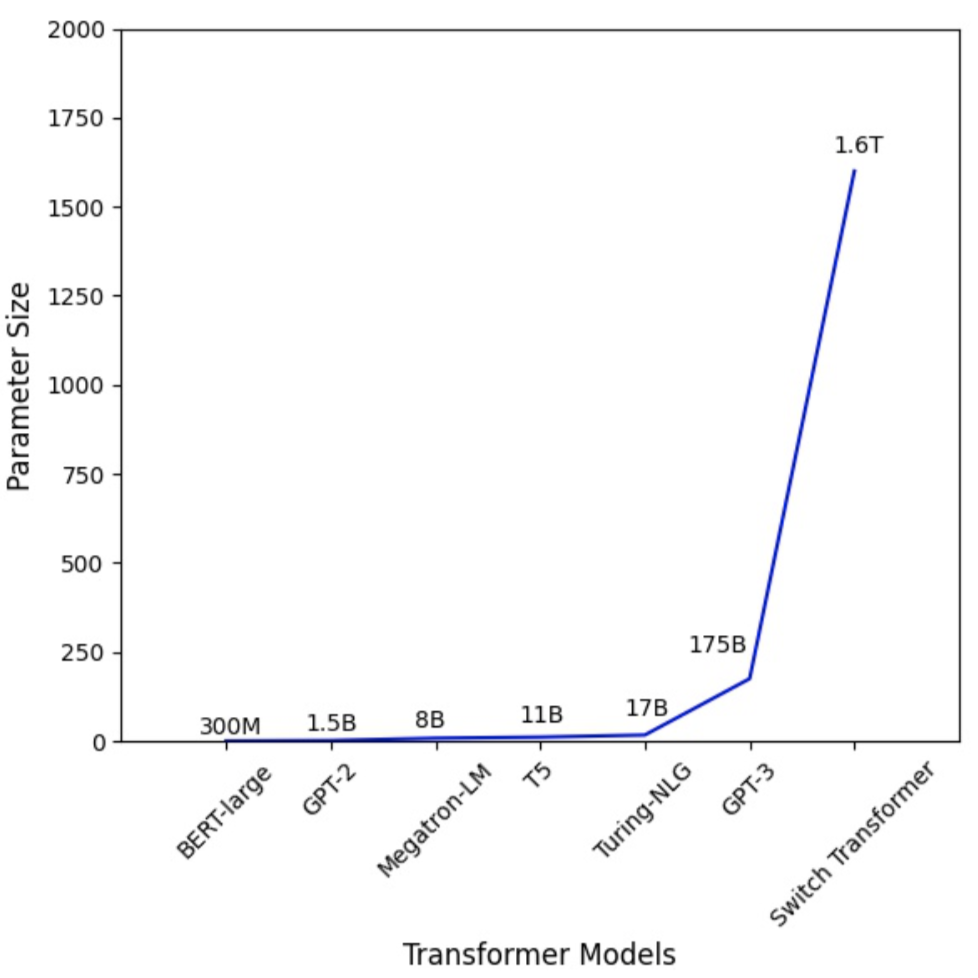
Figure 1: the Parameter Number of Transformer Models Increases Dramatically.

Large Transformer models [4][5] have powered accuracy breakthroughs in both natural language processing and computer vision. GPT-3 [4] hit a new record high accuracy for nearly all NLP tasks. Vision Transformer (ViT) [3] also achieved 89% top-1 accuracy in ImageNet, outperforming state-of-the-art convolutional networks ResNet-152 and EfficientNet. To tackle the growth in model sizes, researchers have proposed various distributed training techniques, including parameter servers [6][7][8], pipeline parallelism [9][10][11][12], intra-layer parallelism [13][14][15], and zero redundancy data-parallel [16].

Existing distributed training solutions, however, only study scenarios where all model weights are required to be optimized throughout the training (i.e., computation and communication overhead remains relatively static over different iterations). Recent works on progressive training suggest that parameters in neural networks can be trained dynamically:

  • Freeze Training: Singular Vector Canonical Correlation Analysis for Deep Learning Dynamics and Interpretability. NeurIPS 2017
  • Efficient Training of BERT by Progressively Stacking. ICML 2019
  • Accelerating Training of Transformer-Based Language Models with Progressive Layer Dropping. NeurIPS 2020.
  • On the Transformer Growth for Progressive BERT Training. NACCL 2021

Freeze Training

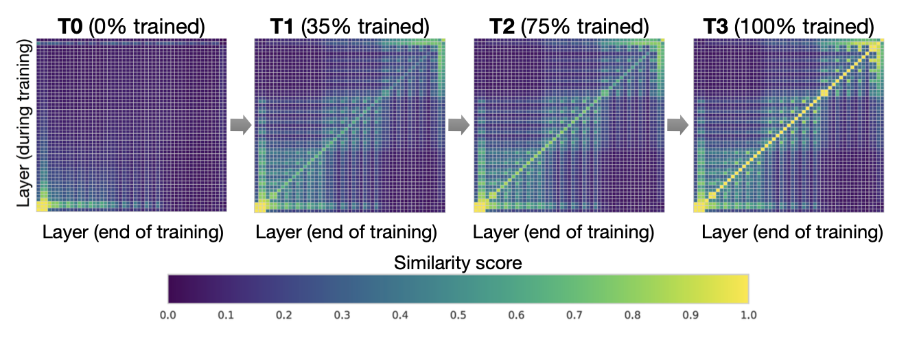
Figure 2. Interpretable Freeze Training: DNNs converge bottom-up (Results on CIFAR10 using ResNet). Each pane shows layer-by-layer similarity using SVCCA [17][18]

For example, in freeze training [17][18], neural networks usually converge from the bottom-up (i.e., not all layers need to be trained all the way through training). Figure 2 shows an example of how weights gradually stabilize during training in this approach. This observation motivates us to utilize freeze training for distributed training of Transformer models to accelerate training by dynamically allocating resources to focus on a shrinking set of active layers. Such a layer freezing strategy is especially pertinent to pipeline parallelism, as excluding consecutive bottom layers from the pipeline can reduce computation, memory, and communication overhead.


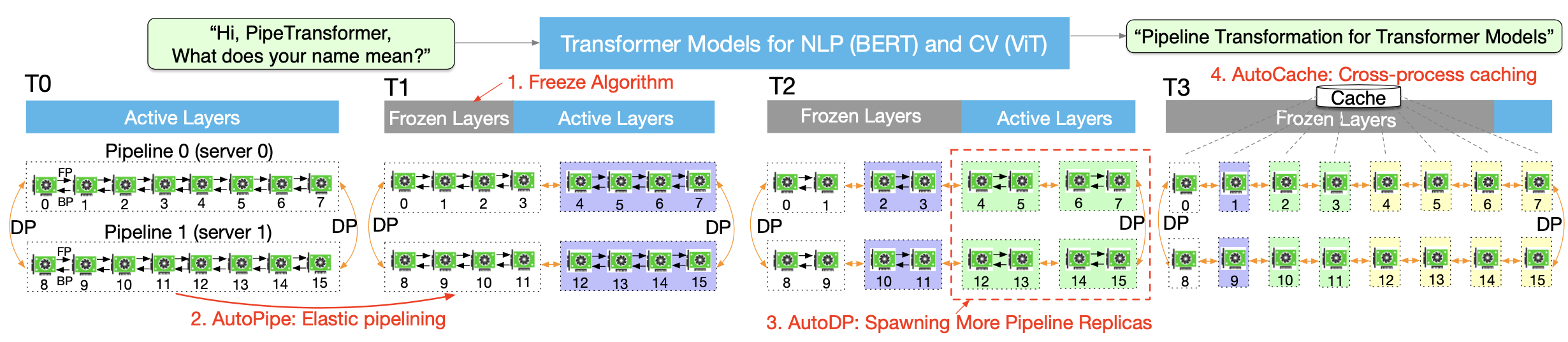
Figure 3. The process of PipeTransformer’s automated and elastic pipelining to accelerate distributed training of Transformer models

We propose PipeTransformer, an elastic pipelining training acceleration framework that automatically reacts to frozen layers by dynamically transforming the scope of the pipelined model and the number of pipeline replicas. To the best of our knowledge, this is the first paper that studies layer freezing in the context of both pipeline and data-parallel training. Figure 3 demonstrates the benefits of such a combination. First, by excluding frozen layers from the pipeline, the same model can be packed into fewer GPUs, leading to both fewer cross-GPU communications and smaller pipeline bubbles. Second, after packing the model into fewer GPUs, the same cluster can accommodate more pipeline replicas, increasing the width of data parallelism. More importantly, the speedups acquired from these two benefits are multiplicative rather than additive, further accelerating the training.

The design of PipeTransformer faces four major challenges. First, the freeze algorithm must make on-the-fly and adaptive freezing decisions; however, existing work [17][18] only provides a posterior analysis tool. Second, the efficiency of pipeline re-partitioning results is influenced by multiple factors, including partition granularity, cross-partition activation size, and the chunking (the number of micro-batches) in mini-batches, which require reasoning and searching in a large solution space. Third, to dynamically introduce additional pipeline replicas, PipeTransformer must overcome the static nature of collective communications and avoid potentially complex cross-process messaging protocols when onboarding new processes (one pipeline is handled by one process). Finally, caching can save time for repeated forward propagation of frozen layers, but it must be shared between existing pipelines and newly added ones, as the system cannot afford to create and warm up a dedicated cache for each replica.

Freeze Training

Figure 4: An Animation to Show the Dynamics of PipeTransformer

As shown in the animation (Figure 4), PipeTransformer is designed with four core building blocks to address the aforementioned challenges. First, we design a tunable and adaptive algorithm to generate signals that guide the selection of layers to freeze over different iterations (Freeze Algorithm). Once triggered by these signals, our elastic pipelining module (AutoPipe), then packs the remaining active layers into fewer GPUs by taking both activation sizes and variances of workloads across heterogeneous partitions (frozen layers and active layers) into account. It then splits a mini-batch into an optimal number of micro-batches based on prior profiling results for different pipeline lengths. Our next module, AutoDP, spawns additional pipeline replicas to occupy freed-up GPUs and maintains hierarchical communication process groups to attain dynamic membership for collective communications. Our final module, AutoCache, efficiently shares activations across existing and new data-parallel processes and automatically replaces stale caches during transitions.

Overall, PipeTransformer combines the Freeze Algorithm, AutoPipe, AutoDP, and AutoCache modules to provide a significant training speedup.
We evaluate PipeTransformer using Vision Transformer (ViT) on ImageNet and BERT on GLUE and SQuAD datasets. Our results show that PipeTransformer attains up to 2.83-fold speedup without losing accuracy. We also provide various performance analyses for a more comprehensive understanding of our algorithmic and system-wise design.
Finally, we have also developed open-source flexible APIs for PipeTransformer, which offer a clean separation among the freeze algorithm, model definitions, and training accelerations, allowing for transferability to other algorithms that require similar freezing strategies.

Overall Design

Suppose we aim to train a massive model in a distributed training system where the hybrid of pipelined model parallelism and data parallelism is used to target scenarios where either the memory of a single GPU device cannot hold the model, or if loaded, the batch size is small enough to avoid running out of memory. More specifically, we define our settings as follows:

Training task and model definition. We train Transformer models (e.g., Vision Transformer, BERT on large-scale image or text datasets. The Transformer model has layers, in which the th layer is composed of a forward computation function and a corresponding set of parameters.

Training infrastructure. Assume the training infrastructure contains a GPU cluster that has GPU servers (i.e. nodes). Each node has GPUs. Our cluster is homogeneous, meaning that each GPU and server have the same hardware configuration. Each GPU’s memory capacity is . Servers are connected by a high bandwidth network interface such as InfiniBand interconnect.

Pipeline parallelism. In each machine, we load a model into a pipeline which has partitions ( also represents the pipeline length). The th partition consists of consecutive layers. We assume each partition is handled by a single GPU device. , meaning that we can build multiple pipelines for multiple model replicas in a single machine. We assume all GPU devices in a pipeline belonging to the same machine. Our pipeline is a synchronous pipeline, which does not involve stale gradients, and the number of micro-batches is . In the Linux OS, each pipeline is handled by a single process. We refer the reader to GPipe [10] for more details.

Data parallelism. DDP is a cross-machine distributed data-parallel process group within parallel workers. Each worker is a pipeline replica (a single process). The th worker’s index (ID) is rank . For any two pipelines in DDP, they can belong to either the same GPU server or different GPU servers, and they can exchange gradients with the AllReduce algorithm.

Under these settings, our goal is to accelerate training by leveraging freeze training, which does not require all layers to be trained throughout the duration of the training. Additionally, it may help save computation, communication, memory cost, and potentially prevent overfitting by consecutively freezing layers. However, these benefits can only be achieved by overcoming the four challenges of designing an adaptive freezing algorithm, dynamical pipeline re-partitioning, efficient resource reallocation, and cross-process caching, as discussed in the introduction.

Overview

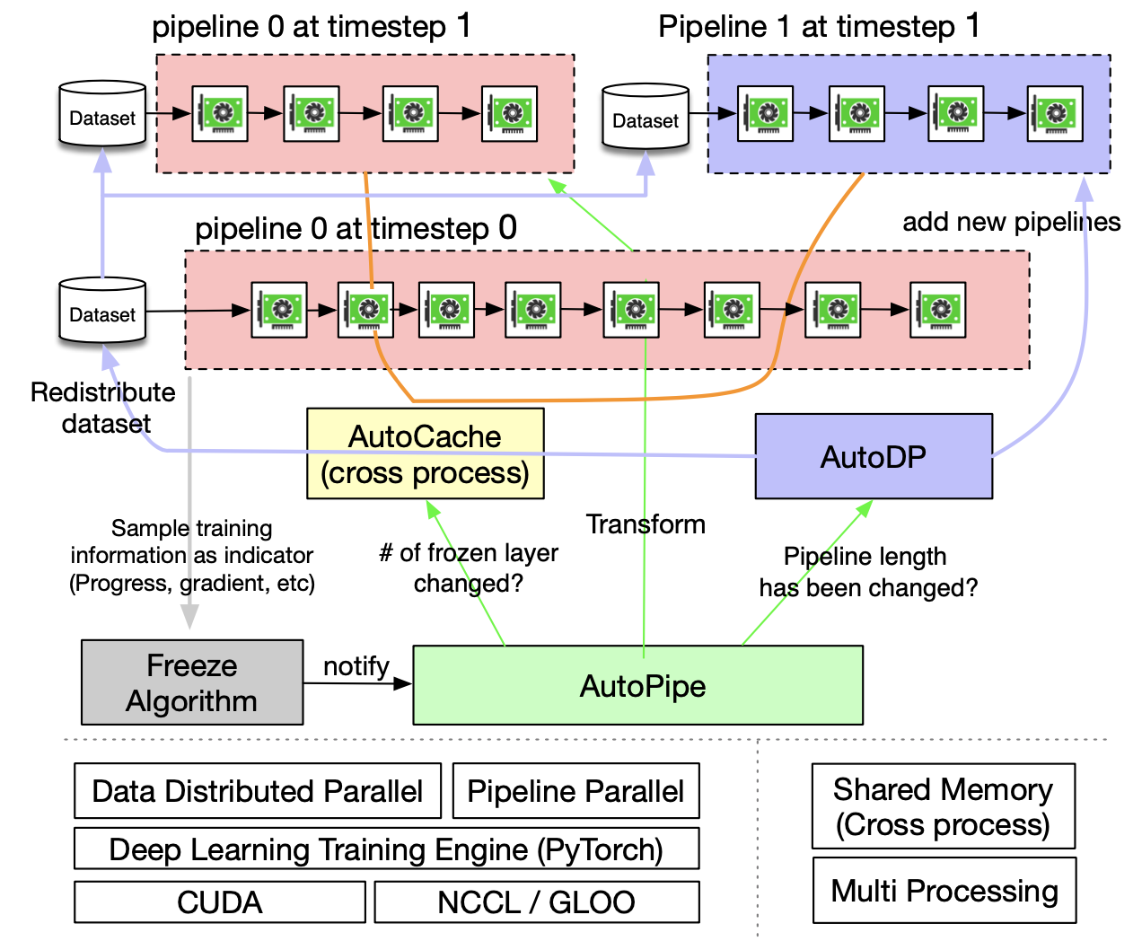
Figure 5. Overview of PipeTransformer Training System

PipeTransformer co-designs an on-the-fly freeze algorithm and an automated elastic pipelining training system that can dynamically transform the scope of the pipelined model and the number of pipeline replicas. The overall system architecture is illustrated in Figure 5. To support PipeTransformer’s elastic pipelining, we maintain a customized version of PyTorch Pipeline. For data parallelism, we use PyTorch DDP as a baseline. Other libraries are standard mechanisms of an operating system (e.g.,multi-processing) and thus avoid specialized software or hardware customization requirements. To ensure the generality of our framework, we have decoupled the training system into four core components: freeze algorithm, AutoPipe, AutoDP, and AutoCache. The freeze algorithm (grey) samples indicators from the training loop and makes layer-wise freezing decisions, which will be shared with AutoPipe (green). AutoPipe is an elastic pipeline module that speeds up training by excluding frozen layers from the pipeline and packing the active layers into fewer GPUs (pink), leading to both fewer cross-GPU communications and smaller pipeline bubbles. Subsequently, AutoPipe passes pipeline length information to AutoDP (purple), which then spawns more pipeline replicas to increase data-parallel width, if possible. The illustration also includes an example in which AutoDP introduces a new replica (purple). AutoCache (orange edges) is a cross-pipeline caching module, as illustrated by connections between pipelines. The source code architecture is aligned with Figure 5 for readability and generality.

Implementation Using PyTorch APIs

As can be seen from Figure 5, PipeTransformers contain four components: Freeze Algorithm, AutoPipe, AutoDP, and AutoCache. Among them, AutoPipe and AutoDP relies on PyTorch DDP (torch.nn.parallel.DistributedDataParallel) [1] and Pipeline (torch.distributed.pipeline), respectively. In this blog, we only highlight the key implementation details of AutoPipe and AutoDP. For details of Freeze Algorithm and AutoCache, please refer to our paper.

AutoPipe: Elastic Pipelining

AutoPipe can accelerate training by excluding frozen layers from the pipeline and packing the active layers into fewer GPUs. This section elaborates on the key components of AutoPipe that dynamically 1) partition pipelines, 2) minimize the number of pipeline devices, and 3) optimize mini-batch chunk size accordingly.

Basic Usage of PyTorch Pipeline

Before diving into details of AutoPipe, let us warm up the basic usage of PyTorch Pipeline (torch.distributed.pipeline.sync.Pipe, see this tutorial). More specially, we present a simple example to understand the design of Pipeline in practice:

# Step 1: build a model including two linear layers
fc1 = nn.Linear(16, 8).cuda(0)
fc2 = nn.Linear(8, 4).cuda(1)

# Step 2: wrap the two layers with nn.Sequential
model = nn.Sequential(fc1, fc2)

# Step 3: build Pipe (torch.distributed.pipeline.sync.Pipe)
model = Pipe(model, chunks=8)

# do training/inference
input = torch.rand(16, 16).cuda(0)
output_rref = model(input)

In this basic example, we can see that before initializing Pipe, we need to partition the model nn.Sequential into multiple GPU devices and set optimal chunk number (chunks). Balancing computation time across partitions is critical to pipeline training speed, as skewed workload distributions across stages can lead to stragglers and forcing devices with lighter workloads to wait. The chunk number may also have a non-trivial influence on the throughput of the pipeline.

Balanced Pipeline Partitioning

In dynamic training system such as PipeTransformer, maintaining optimally balanced partitions in terms of parameter numbers does not guarantee the fastest training speed because other factors also play a crucial role:


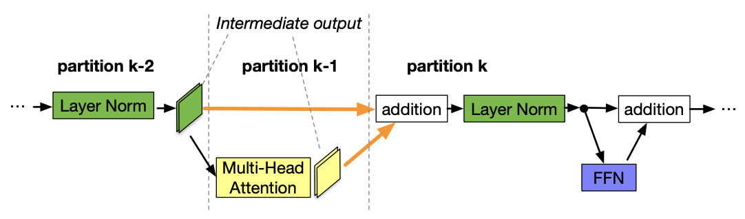
Figure 6. The partition boundary is in the middle of a skip connection

  1. Cross-partition communication overhead. Placing a partition boundary in the middle of a skip connection leads to additional communications since tensors in the skip connection must now be copied to a different GPU. For example, with BERT partitions in Figure 6, partition must take intermediate outputs from both partition and partition . In contrast, if the boundary is placed after the addition layer, the communication overhead between partition and is visibly smaller. Our measurements show that having cross-device communication is more expensive than having slightly imbalanced partitions (see the Appendix in our paper). Therefore, we do not consider breaking skip connections (highlighted separately as an entire attention layer and MLP layer in green color at line 7 in Algorithm 1.

  2. Frozen layer memory footprint. During training, AutoPipe must recompute partition boundaries several times to balance two distinct types of layers: frozen layers and active layers. The frozen layer’s memory cost is a fraction of that inactive layer, given that the frozen layer does not need backward activation maps, optimizer states, and gradients. Instead of launching intrusive profilers to obtain thorough metrics on memory and computational cost, we define a tunable cost factor to estimate the memory footprint ratio of a frozen layer over the same active layer. Based on empirical measurements in our experimental hardware, we set it to .


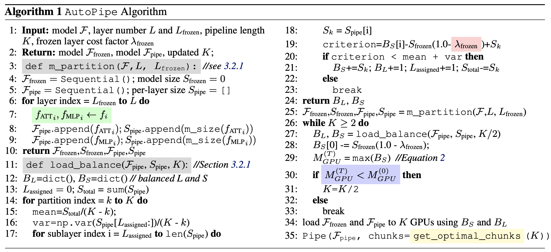
Based on the above two considerations, AutoPipe balances pipeline partitions based on parameter sizes. More specifically, AutoPipe uses a greedy algorithm to allocate all frozen and active layers to evenly distribute partitioned sublayers into GPU devices. Pseudocode is described as the load_balance() function in Algorithm 1. The frozen layers are extracted from the original model and kept in a separate model instance in the first device of a pipeline.

Note that the partition algorithm employed in this paper is not the only option; PipeTransformer is modularized to work with any alternatives.

Pipeline Compression

Pipeline compression helps to free up GPUs to accommodate more pipeline replicas and reduce the number of cross-device communications between partitions. To determine the timing of compression, we can estimate the memory cost of the largest partition after compression, and then compare it with that of the largest partition of a pipeline at timestep . To avoid extensive memory profiling, the compression algorithm uses the parameter size as a proxy for the training memory footprint. Based on this simplification, the criterion of pipeline compression is as follows:


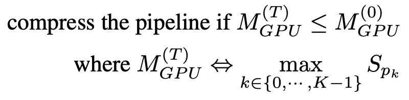
Once the freeze notification is received, AutoPipe will always attempt to divide the pipeline length by 2 (e.g., from 8 to 4, then 2). By using as the input, the compression algorithm can verify if the result satisfies the criterion in Equation (1). Pseudocode is shown in lines 25-33 in Algorithm 1. Note that this compression makes the acceleration ratio exponentially increase during training, meaning that if a GPU server has a larger number of GPUs (e.g., more than 8), the acceleration ratio will be further amplified.


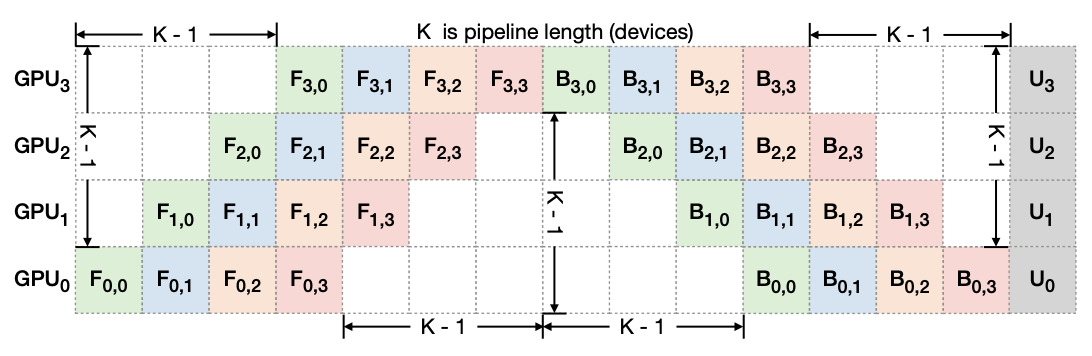
Figure 7. Pipeline Bubble: , and denote forward, backward, and the optimizer update of micro-batch on device , respectively. The total bubble size in each iteration is times per micro-batch forward and backward cost.

Additionally, such a technique can also speed up training by shrinking the size of pipeline bubbles. To explain bubble sizes in a pipeline, Figure 7 depicts how 4 micro-batches run through a 4-device pipeline . In general, the total bubble size is times per micro-batch forward and backward cost. Therefore, it is clear that shorter pipelines have smaller bubble sizes.

Dynamic Number of Micro-Batches

Prior pipeline parallel systems use a fixed number of micro-batches per mini-batch ( ). GPipe suggests , where is the number of partitions (pipeline length). However, given that PipeTransformer dynamically configures , we find it to be sub-optimal to maintain a static during training. Moreover, when integrated with DDP, the value of also has an impact on the efficiency of DDP gradient synchronizations. Since DDP must wait for the last micro-batch to finish its backward computation on a parameter before launching its gradient synchronization, finer micro-batches lead to a smaller overlap between computation and communication. Hence, instead of using a static value, PipeTransformer searches for optimal on the fly in the hybrid of DDP environment by enumerating values ranging from to . For a specific training environment, the profiling needs only to be done once (see Algorithm 1 line 35).

For the complete source code, please refer to https://github.com/Distributed-AI/PipeTransformer/blob/master/pipe_transformer/pipe/auto_pipe.py.

AutoDP: Spawning More Pipeline Replicas

As AutoPipe compresses the same pipeline into fewer GPUs, AutoDP can automatically spawn new pipeline replicas to increase data-parallel width.

Despite the conceptual simplicity, subtle dependencies on communications and states require careful design. The challenges are threefold:

  1. DDP Communication: Collective communications in PyTorch DDP requires static membership, which prevents new pipelines from connecting with existing ones;

  2. State Synchronization: newly activated processes must be consistent with existing pipelines in the training progress (e.g., epoch number and learning rate), weights and optimizer states, the boundary of frozen layers, and pipeline GPU range;

  3. Dataset Redistribution: the dataset should be re-balanced to match a dynamic number of pipelines. This not only avoids stragglers but also ensures that gradients from all DDP processes are equally weighted.


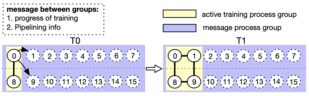
Figure 8. AutoDP: handling dynamical data-parallel with messaging between double process groups (Process 0-7 belong to machine 0, while process 8-15 belong to machine 1)

To tackle these challenges, we create double communication process groups for DDP. As in the example shown in Figure 8, the message process group (purple) is responsible for light-weight control messages and covers all processes, while the active training process group (yellow) only contains active processes and serves as a vehicle for heavy-weight tensor communications during training. The message group remains static, whereas the training group is dismantled and reconstructed to match active processes.
In T0, only processes 0 and 8 are active. During the transition to T1, process 0 activates processes 1 and 9 (newly added pipeline replicas) and synchronizes necessary information mentioned above using the message group. The four active processes then form a new training group, allowing static collective communications adaptive to dynamic memberships.
To redistribute the dataset, we implement a variant of DistributedSampler that can seamlessly adjust data samples to match the number of active pipeline replicas.

The above design also naturally helps to reduce DDP communication overhead. More specifically, when transitioning from T0 to T1, processes 0 and 1 destroy the existing DDP instances, and active processes construct a new DDP training group using a cached pipelined model (AutoPipe stores frozen model and cached model separately).

We use the following APIs to implement the design above.

import torch.distributed as dist
from torch.nn.parallel import DistributedDataParallel as DDP

# initialize the process group (this must be called in the initialization of PyTorch DDP)
dist.init_process_group(init_method='tcp://' + str(self.config.master_addr) + ':' +
str(self.config.master_port), backend=Backend.GLOO, rank=self.global_rank, world_size=self.world_size)
...

# create active process group (yellow color)
self.active_process_group = dist.new_group(ranks=self.active_ranks, backend=Backend.NCCL, timeout=timedelta(days=365))
...

# create message process group (yellow color)
self.comm_broadcast_group = dist.new_group(ranks=[i for i in range(self.world_size)], backend=Backend.GLOO, timeout=timedelta(days=365))
...

# create DDP-enabled model when the number of data-parallel workers is changed. Note:
# 1. The process group to be used for distributed data all-reduction.
If None, the default process group, which is created by torch.distributed.init_process_group, will be used.
In our case, we set it as self.active_process_group
# 2. device_ids should be set when the pipeline length = 1 (the model resides on a single CUDA device).

self.pipe_len = gpu_num_per_process
if gpu_num_per_process > 1:
    model = DDP(model, process_group=self.active_process_group, find_unused_parameters=True)
else:
    model = DDP(model, device_ids=[self.local_rank], process_group=self.active_process_group, find_unused_parameters=True)

# to broadcast message among processes, we use dist.broadcast_object_list
def dist_broadcast(object_list, src, group):
    """Broadcasts a given object to all parties."""
    dist.broadcast_object_list(object_list, src, group=group)
    return object_list

For the complete source code, please refer to https://github.com/Distributed-AI/PipeTransformer/blob/master/pipe_transformer/dp/auto_dp.py.

Experiments

This section first summarizes experiment setups and then evaluates PipeTransformer using computer vision and natural language processing tasks.

Hardware. Experiments were conducted on 2 identical machines connected by InfiniBand CX353A (GB/s), where each machine is equipped with 8 NVIDIA Quadro RTX 5000 (16GB GPU memory). GPU-to-GPU bandwidth within a machine (PCI 3.0, 16 lanes) is GB/s.

Implementation. We used PyTorch Pipe as a building block. The BERT model definition, configuration, and related tokenizer are from HuggingFace 3.5.0. We implemented Vision Transformer using PyTorch by following its TensorFlow implementation. More details can be found in our source code.

Models and Datasets. Experiments employ two representative Transformers in CV and NLP: Vision Transformer (ViT) and BERT. ViT was run on an image classification task, initialized with pre-trained weights on ImageNet21K and fine-tuned on ImageNet and CIFAR-100. BERT was run on two tasks, text classification on the SST-2 dataset from the General Language Understanding Evaluation (GLUE) benchmark, and question answering on the SQuAD v1.1 Dataset (Stanford Question Answering), which is a collection of 100k crowdsourced question/answer pairs.

Training Schemes. Given that large models normally would require thousands of GPU-days {emph{e.g.}, GPT-3) if trained from scratch, fine-tuning downstream tasks using pre-trained models has become a trend in CV and NLP communities. Moreover, PipeTransformer is a complex training system that involves multiple core components. Thus, for the first version of PipeTransformer system development and algorithmic research, it is not cost-efficient to develop and evaluate from scratch using large-scale pre-training. Therefore, the experiments presented in this section focuses on pre-trained models. Note that since the model architectures in pre-training and fine-tuning are the same, PipeTransformer can serve both. We discussed pre-training results in the Appendix.

Baseline. Experiments in this section compare PipeTransformer to the state-of-the-art framework, a hybrid scheme of PyTorch Pipeline (PyTorch’s implementation of GPipe) and PyTorch DDP. Since this is the first paper that studies accelerating distributed training by freezing layers, there are no perfectly aligned counterpart solutions yet.

Hyper-parameters. Experiments use ViT-B/16 (12 transformer layers, input patch size) for ImageNet and CIFAR-100, BERT-large-uncased (24 layers) for SQuAD 1.1, and BERT-base-uncased (12 layers) for SST-2. With PipeTransformer, ViT and BERT training can set the per-pipeline batch size to around 400 and 64, respectively. Other hyperparameters (e.g., epoch, learning rate) for all experiments are presented in Appendix.

Overall Training Acceleration


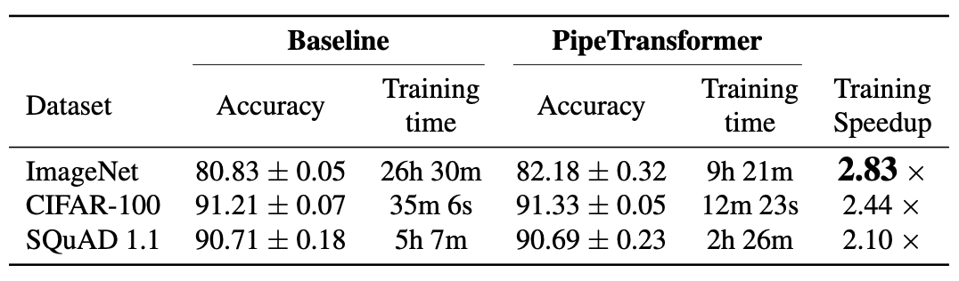
We summarize the overall experimental results in the table above. Note that the speedup we report is based on a conservative value that can obtain comparable or even higher accuracy. A more aggressive (, ) can obtain a higher speedup but may lead to a slight loss in accuracy. Note that the model size of BERT (24 layers) is larger than ViT-B/16 (12 layers), thus it takes more time for communication.

Performance Analysis

Speedup Breakdown

This section presents evaluation results and analyzes the performance of different components in autopipe. More experimental results can be found in the Appendix.


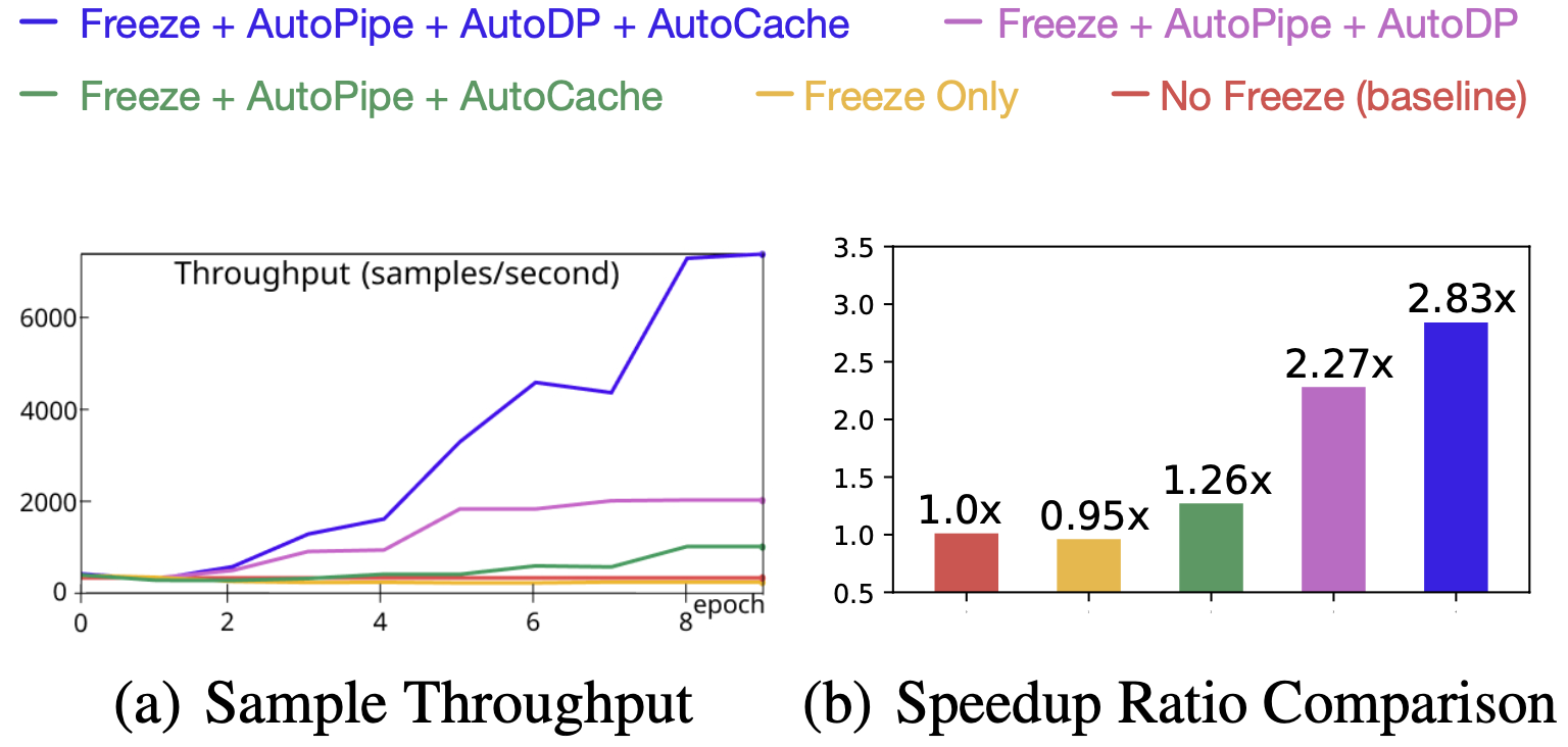
Figure 9. Speedup Breakdown (ViT on ImageNet)

To understand the efficacy of all four components and their impacts on training speed, we experimented with different combinations and used their training sample throughput (samples/second) and speedup ratio as metrics. Results are illustrated in Figure 9. Key takeaways from these experimental results are:

  1. the main speedup is the result of elastic pipelining which is achieved through the joint use of AutoPipe and AutoDP;
  2. AutoCache’s contribution is amplified by AutoDP;
  3. freeze training alone without system-wise adjustment even downgrades the training speed.

Tuning in Freezing Algorithm


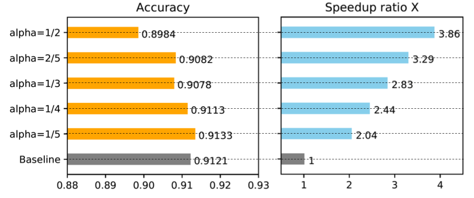
Figure 10. Tuning in Freezing Algorithm

We ran experiments to show how the in the freeze algorithms influences training speed. The result clearly demonstrates that a larger (excessive freeze) leads to a greater speedup but suffers from a slight performance degradation. In the case shown in Figure 10, where , freeze training outperforms normal training and obtains a -fold speedup. We provide more results in the Appendix.

Optimal Chunks in the elastic pipeline


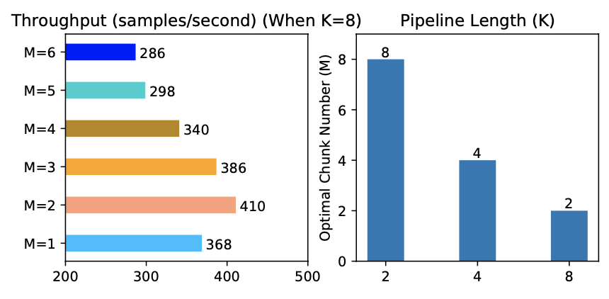
Figure 11. Optimal chunk number in the elastic pipeline

We profiled the optimal number of micro-batches for different pipeline lengths . Results are summarized in Figure 11. As we can see, different values lead to different optimal , and the throughput gaps across different M values are large (as shown when ), which confirms the necessity of an anterior profiler in elastic pipelining.

Understanding the Timing of Caching


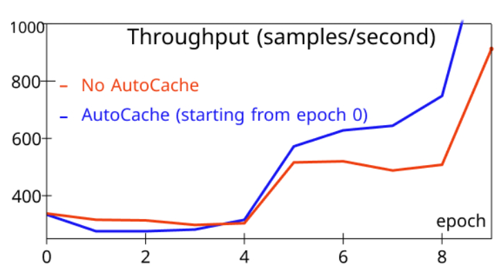
Figure 12. the timing of caching

To evaluate AutoCache, we compared the sample throughput of training that activates AutoCache from epoch (blue) with the training job without AutoCache (red). Figure 12 shows that enabling caching too early can slow down training, as caching can be more expensive than the forward propagation on a small number of frozen layers. After more layers are frozen, caching activations clearly outperform the corresponding forward propagation. As a result, AutoCache uses a profiler to determine the proper timing to enable caching. In our system, for ViT (12 layers), caching starts from 3 frozen layers, while for BERT (24 layers), caching starts from 5 frozen layers.

For more detailed experimental analysis, please refer to our paper.

Summarization

This blog introduces PipeTransformer, a holistic solution that combines elastic pipeline-parallel and data-parallel for distributed training using PyTorch Distributed APIs. More specifically, PipeTransformer incrementally freezes layers in the pipeline, packs remaining active layers into fewer GPUs, and forks more pipeline replicas to increase the data-parallel width. Evaluations on ViT and BERT models show that compared to the state-of-the-art baseline, PipeTransformer attains up to 2.83× speedups without accuracy loss.

Reference

[1] Li, S., Zhao, Y., Varma, R., Salpekar, O., Noordhuis, P., Li,T., Paszke, A., Smith, J., Vaughan, B., Damania, P., et al. Pytorch Distributed: Experiences on Accelerating Dataparallel Training. Proceedings of the VLDB Endowment,13(12), 2020

[2] Devlin, J., Chang, M. W., Lee, K., and Toutanova, K. BERT: Pre-training of Deep Bidirectional Transformers for Language Understanding. In NAACL-HLT, 2019

[3] Dosovitskiy, A., Beyer, L., Kolesnikov, A., Weissenborn, D., Zhai, X., Unterthiner, T., Dehghani, M., Minderer, M., Heigold, G., Gelly, S., et al. An image is Worth 16×16 words: Transformers for Image Recognition at Scale.

[4] Brown, T. B., Mann, B., Ryder, N., Subbiah, M., Kaplan, J., Dhariwal, P., Neelakantan, A., Shyam, P., Sastry, G., Askell, A., et al. Language Models are Few-shot Learners.

[5] Lepikhin, D., Lee, H., Xu, Y., Chen, D., Firat, O., Huang, Y., Krikun, M., Shazeer, N., and Chen, Z. Gshard: Scaling Giant Models with Conditional Computation and Automatic Sharding.

[6] Li, M., Andersen, D. G., Park, J. W., Smola, A. J., Ahmed, A., Josifovski, V., Long, J., Shekita, E. J., and Su, B. Y. Scaling Distributed Machine Learning with the Parameter Server. In 11th {USENIX} Symposium on Operating Systems Design and Implementation ({OSDI} 14), pp. 583–598, 2014.

[7] Jiang, Y., Zhu, Y., Lan, C., Yi, B., Cui, Y., and Guo, C. A Unified Architecture for Accelerating Distributed DNN Training in Heterogeneous GPU/CPU Clusters. In 14th USENIX Symposium on Operating Systems Design and Implementation (OSDI 20), pp. 463–479. USENIX Association, November 2020. ISBN 978-1-939133-19- 9.

[8] Kim, S., Yu, G. I., Park, H., Cho, S., Jeong, E., Ha, H., Lee, S., Jeong, J. S., and Chun, B. G. Parallax: Sparsity-aware Data Parallel Training of Deep Neural Networks. In Proceedings of the Fourteenth EuroSys Conference 2019, pp. 1–15, 2019.

[9] Kim, C., Lee, H., Jeong, M., Baek, W., Yoon, B., Kim, I., Lim, S., and Kim, S. TorchGPipe: On-the-fly Pipeline Parallelism for Training Giant Models.

[10] Huang, Y., Cheng, Y., Bapna, A., Firat, O., Chen, M. X., Chen, D., Lee, H., Ngiam, J., Le, Q. V., Wu, Y., et al. Gpipe: Efficient Training of Giant Neural Networks using Pipeline Parallelism.

[11] Park, J. H., Yun, G., Yi, C. M., Nguyen, N. T., Lee, S., Choi, J., Noh, S. H., and ri Choi, Y. Hetpipe: Enabling Large DNN Training on (whimpy) Heterogeneous GPU Clusters through Integration of Pipelined Model Parallelism and Data Parallelism. In 2020 USENIX Annual Technical Conference (USENIX ATC 20), pp. 307–321. USENIX Association, July 2020. ISBN 978-1-939133- 14-4.

[12] Narayanan, D., Harlap, A., Phanishayee, A., Seshadri, V., Devanur, N. R., Ganger, G. R., Gibbons, P. B., and Zaharia, M. Pipedream: Generalized Pipeline Parallelism for DNN Training. In Proceedings of the 27th ACM Symposium on Operating Systems Principles, SOSP ’19, pp. 1–15, New York, NY, USA, 2019. Association for Computing Machinery. ISBN 9781450368735. doi: 10.1145/3341301.3359646.

[13] Lepikhin, D., Lee, H., Xu, Y., Chen, D., Firat, O., Huang, Y., Krikun, M., Shazeer, N., and Chen, Z. Gshard: Scaling Giant Models with Conditional Computation and Automatic Sharding.

[14] Shazeer, N., Cheng, Y., Parmar, N., Tran, D., Vaswani, A., Koanantakool, P., Hawkins, P., Lee, H., Hong, M., Young, C., Sepassi, R., and Hechtman, B. Mesh-Tensorflow: Deep Learning for Supercomputers. In Bengio, S., Wallach, H., Larochelle, H., Grauman, K., Cesa-Bianchi, N., and Garnett, R. (eds.), Advances in Neural Information Processing Systems, volume 31, pp. 10414–10423. Curran Associates, Inc., 2018.

[15] Shoeybi, M., Patwary, M., Puri, R., LeGresley, P., Casper, J., and Catanzaro, B. Megatron-LM: Training Multi-billion Parameter Language Models using Model Parallelism.

[16] Rajbhandari, S., Rasley, J., Ruwase, O., and He, Y. ZERO: Memory Optimization towards Training a Trillion Parameter Models.

[17] Raghu, M., Gilmer, J., Yosinski, J., and Sohl Dickstein, J. Svcca: Singular Vector Canonical Correlation Analysis for Deep Learning Dynamics and Interpretability. In NIPS, 2017.

[18] Morcos, A., Raghu, M., and Bengio, S. Insights on Representational Similarity in Neural Networks with Canonical Correlation. In Bengio, S., Wallach, H., Larochelle, H., Grauman, K., Cesa-Bianchi, N., and Garnett, R. (eds.), Advances in Neural Information Processing Systems 31, pp. 5732–5741. Curran Associates, Inc., 2018.

Read More

What it’s like being a senior researcher at Facebook Core Data Science

Facebook’s Core Data Science (CDS) team is pushing the envelope of what’s possible by exploring and solving novel challenges in science and technology. Senior researchers bring experience across disciplines that range from computer science and statistics to political science and sociology, using data to drive decision-making across product teams. “Our data supports product development across Facebook, and we see our results come to life as optimization, new features, and programs,” explains Shawndra Hill, CDS Research Scientist and Manager.

The unique cross-functional nature of the CDS team and available growth opportunities for senior researchers help set Facebook apart from academic research and other technology companies. Three team members share more about their areas of focus, what a day on the CDS team is like, and their best advice for helping senior researchers succeed.

Staying curious while using data to drive decisions

Ahmed Medhat is a post-graduate of Oxford University, where he studied collaborative behavior in online networks. He joined Facebook five years ago as a staff data scientist before transitioning into a research scientist role with the CDS team.

“Working as part of Facebook Data for Good, my current focus is on creating privacy-safe data sets and tools for addressing some of the world’s greatest humanitarian issues,” Ahmed explains. “Working on this as a research scientist, I’m challenged to find ways to help communities across the world that are both complementary to other resources provided by humanitarian organizations and as scalable and uniform as possible across different geographical regions. While with research in academia it can take some time to sense the real-world impact of one’s research, at Facebook we have a unique opportunity to see the direct impact our work has on the wider research community more quickly. For example, we created tools that can help organizations respond to the Covid-19 pandemic, such as looking at how populations are responding to physical distancing measures, to inform researchers and public health experts.”

Ahmed and his teams are driven by the opportunity to drive life-changing projects and offer something new. “Our work calls for a lot of autonomy and self-accountability,” he shares. “Staying curious and bringing a fresh perspective is important. For those interested in joining the CDS team as a senior researcher, my advice is to demonstrate the unique skills and perspectives that you can bring to Facebook. We also love to see adaptability and the ability to wear different hats. At this level, you’re expected to see beyond the daily minutiae of analysis and code writing, towards work that broadly impacts the company’s product direction and pushes the state of the art in your research area.”

Using passion to drive your research and career path

The CDS team’s Shawndra Hill is also a part-time senior marketing lecturer at Columbia University. She has a PhD in management information systems from NYU Stern School of Business, and prior to her role at Facebook, she was a Senior Principal Researcher at Microsoft Research and a professor at the Wharton School of the University of Pennsylvania. As a manager, Shawndra oversees projects while empowering her team to grow and succeed. Her current research is focused on deriving value from social networks and online behaviors for a range of Facebook’s business applications — specifically for advertising applications that bring people closer to the things they want and need.

“At the senior level, having strong project management skills is critical,” says Shawndra, in reference to her ability to split her time between leadership and individual project work. “During the interview process with Facebook, I saw limitless growth opportunities within the company because of the scale of data science problems, and was also specific about my desire to grow into a management position. With the support and opportunities available within Facebook Research, I was able to reach my goals of leading Facebook scale advertising projects as an individual contributor and becoming a manager within a year.”

Now, Shawndra says, leading a passionate team of researchers is one of her favorite parts of her role. “We’re collaborating in a fast-paced environment. People at Facebook want to translate research into product impact in a short amount of time, and for a researcher, that’s an exciting opportunity that doesn’t often exist in other career paths like academia. To succeed in this field, I suggest identifying the areas you’re most interested in and using that knowledge to find projects at the intersection of your passion and company priorities. From there, you’ll be well positioned to develop a relevant specialty for Facebook and prioritize projects for company impact. As a senior researcher, your experience and deep understanding of relevant research methodologies will add value to teams while also helping them to balance rigor with getting things done. My advice for other senior scientists is to be consistently excellent, someone others want to go to, the person they know they can depend on for quality output.”

Exploring every opportunity to find an area of focus

Ami Tavory holds a PhD in information theory from Tel Aviv University and is a Research Scientist on the CDS team. He was struck by Facebook’s collaborative structure upon joining nearly four years ago, and he found his place working closely with several highly skilled product teams, specializing in detecting and preventing fraud with machine learning in F2 (Facebook Financial Services).

“I’ve been continually impressed with how intentional the Research organization is about building and connecting groups,” he shares. “I’ve worked with several product teams, and have been surprised by the level of collaboration and support. This allows me to find several areas and projects that are the best fit for my interests and my experience. ”

Ami highlights the autonomy at Facebook as another unique aspect of being a part of the team, and says that for a senior researcher with deep experience, it’s an empowering benefit. “Take control of your personal path by exploring every opportunity available to you at Facebook,” he explains. “It’s important to find a combination of something you enjoy that also brings value to the team. Once you find this balance, things will naturally fall into place. We have people on our team who have successfully switched between a management track and a more technical path, and vice versa.

I’ve been blown away by the level of people with whom I work; on some occasions, I’ve read published studies only to realize that the authors are actually part of the Facebook team and happy to collaborate. No two days are the same here, and you’ll find endless opportunities to collaborate on solving complex challenges at scale.”

Interested in learning more about the CDS team? Check out their research team page.

The post What it’s like being a senior researcher at Facebook Core Data Science appeared first on Facebook Research.

Read More

Optimize personalized recommendations for a business metric of your choice with Amazon Personalize

Amazon Personalize now enables you to optimize personalized recommendations for a business metric of your choice, in addition to improving relevance of recommendations for your users. You can define a business metric such as revenue, profit margin, video watch time, or any other numerical attribute of your item catalog to optimize your recommendations. Amazon Personalize automatically learns what is relevant to your users, considers the business metric you’ve defined, and recommends the products or content to your users that benefit your overall business goals. Configuring an additional objective is easy. You select any numerical column in your catalog when creating a new solution in Amazon Personalize via the AWS Management Console or the API, and you’re ready to go.

Amazon Personalize enables you to easily add real-time personalized recommendations to your applications without requiring any ML expertise. With Amazon Personalize, you pay for what you use, with no minimum fees or upfront commitments. You can get started with a simple three-step process, which takes only a few clicks on the console or a few simple API calls. First, point Amazon Personalize to your user data, catalog data, and activity stream of views, clicks, purchases, and so on, in Amazon Simple Storage Service (Amazon S3) or upload using an API call. Second, either via the console or an API call, train a custom, private recommendation model for your data (CreateSolution). Third, retrieve personalized recommendations for any user by creating a campaign and using the GetRecommendations API.

The rest of this post walks you through the suggested best practices for generating recommendations for your business in greater detail.

Streaming movie service use case

In this post, we propose a fictitious streaming movie service, and as part of the service we provide movie recommendations using movie reviews from the MovieLens database. We assume the streaming service’s agreement with content providers requires royalties every time a movie is viewed. For our use case, we assume movies that have royalties that range from $0.00 to $0.10 per title. All things being equal, the streaming service wants to provide recommendations for titles that the subscriber will enjoy, but minimize costs by recommending titles with lower royalty fees.

It’s important to understand that a trade-off is made when including a business objective in recommendations. Placing too much weight on the objective can lead to a loss of opportunities with customers as the recommendations presented become less relevant to user interests. If the objective weight doesn’t impart enough impact on recommendations, the recommendations will still be relevant but may not drive the business outcomes you aim to achieve. By testing the models in real-world environments, you can collect data on the impact the objective has on your results and balance the relevance of the recommendations with your business objective.

Movie dataset

The items dataset from MovieLens has a structure as follows.

ITEM_ID TITLE ROYALTY GENRE
1 Toy Story (1995) 0.01 ANIMATION|CHILDRENS|COMEDY
2 GoldenEye (1995) 0.02 ACTION|ADVENTURE|THRILLER
3 Four Rooms (1995) 0.03 THRILLER
4 Get Shorty (1995) 0.04 ACTION|COMEDY|DRAMA
5 Copycat (1995) 0.05 CRIME|DRAMA|THRILLER

Amazon Personalize objective optimization requires a numerical field to be defined in the item metadata, which is used when considering your business objective. Because Amazon Personalize optimizes for the largest value in the business metric column, simply passing in the royalty amount results in the recommendations driving customers to those movies with the highest royalties. To minimize royalties, we multiply the royalty field by -1, and capture how much the streaming service will spend in royalties to stream the movie.

ITEM_ID TITLE ROYALTY GENRE
1 Toy Story (1995) -0.01 ANIMATION|CHILDRENS|COMEDY
2 GoldenEye (1995) -0.02 ACTION|ADVENTURE|THRILLER
3 Four Rooms (1995) -0.03 THRILLER
4 Get Shorty (1995) -0.04 ACTION|COMEDY|DRAMA
5 Copycat (1995) -0.05 CRIME|DRAMA|THRILLER

In this example, the royalty value ranges from -0.12 to 0. The objective’s value can be an integer or a floating point, and the lowest value is adjusted to zero internally by the service when creating a solution regardless of whether the lowest value is positive or negative. The highest value is adjusted to 1, and other values are interpolated between 0–1, preserving the relative difference between all data points.

For movie recommendations, we use the following schema for the items dataset:

{
    "type": "record",
    "name": "Items",
    "namespace": "com.amazonaws.personalize.schema",
    "fields": [
        {
            "name": "ITEM_ID",
            "type": "string"
        },
        {
            "name": "ROYALTY",
            "type": "float"
        },
        {
            "name": "GENRE",
            "type": [
                "null",
                "string"
              ],
            "categorical": True
        }
    ],
    "version": "1.0"
}

The items dataset includes the mandatory ITEM_ID field, list of genres, and savings fields.

Comparing three solutions

The following diagram illustrates the architecture we use to test the benefits of objective optimization. In this scenario, we use two buckets – Items contains movie data and Interactions contains positive movie reviews. The data from the buckets is loaded into the Amazon Personalize dataset group. Once loaded, three solutions are driven from the two datasets: one solution with objective sensitivity off, a second solution with objective sensitivity set to low, and the third has the objective sensitivity set to high. Each of these solutions drives a corresponding campaign.

After the datasets are loaded in an Amazon Personalize dataset group, we create three solutions to demonstrate the impact of the varied objective optimizations on recommendations. The optimization objective selected when creating an Amazon Personalize solution and can have a sensitivity level set to one of four values: OFF, LOW, MEDIUM, or HIGH. This provides a setting on how much weight to give to the business objective, and in this post we show the impact that these settings can have on recommendation performance. While developing your own models, you should experiment with the sensitivity setting to evaluate what drives the best results for your recommendations. Because the objective optimization maximizes for the business metric, we must select ROYALTY as the objective optimization column.

The following example Python code creates an Amazon Personalize solution:

create_solution_response = personalize.create_solution(
        name = "solution name",
        datasetGroupArn = dataset_group_arn,
        recipeArn = recipe_arn,
        solutionConfig = {
            "optimizationObjective": {
                "itemAttribute": "ROYALTY",
                "objectiveSensitivity":"HIGH"
            }
        }
    )

After the solution versions have been trained, you can compare the offline metrics by calling the DescribeSolutionVersion API or visiting the Amazon Personalize console for each solution version.

Metric no-optimization low-optimization high-optimization
Average rewards-at-k 0.1491 0.1412 0.1686
coverage 0.1884 0.1711 0.1295
MRR-25 0.0769 0.1116 0.0805
NDCG-10 0.0937 0.1 0.0999
NDCG-25 0.14 0.1599 0.1547
NDCG-5 0.0774 0.0722 0.0698
Precision-10 0.027 0.0292 0.0281
Precision-25 0.0229 0.0256 0.0238
Precision-5 0.0337 0.0315 0.027

In the preceding table, larger numbers are better. For coverage, this is the ratio of items that are present in recommendations compared to the total number of items in the dataset (how many items in your catalog are covered by the recommendation generated). To make sure Amazon Personalize recommends a larger portion of your movie catalog, use a model with a higher coverage score.

The average rewards-at-k metric indicates how the solution version performs in achieving your objective. Amazon Personalize calculates this metric by dividing the total rewards generated by interactions (for example, total revenue from clicks) by the total possible rewards from recommendations. The higher the score, the more gains on average per user you can expect from recommendations.

The mean reciprocal rank (MRR) metric measures the relevance of the highest ranked item in the list, and is important for situations where the user is very likely to select the first item recommended. Normalized discounted cumulative gain at k (NDCG-k) measures the relevance of the highest k items, providing the highest weight to the first k in the list. NDCG is useful for measuring effectiveness when multiple recommendations are presented to users, but highest-rated recommendations are more important than lower-rated recommendations. The Precision-k metric measures the number of relevant recommendations in the top k recommendations.

As the solution weighs the objective higher, metrics tend to show lower relevance for users because the model is selecting recommendations based on user behavior data and the business objective. Amazon Personalize provides the ability to control how much influence the objective imparts on recommendations. If the objective provides too much influence, you can expect it to create a poor customer experience because the recommendations stop being relevant to the user. By running an A/B test, you can collect the data needed to deliver the results that best balance relevance and your business objective.

We can retrieve recommendations from the solution versions by creating an Amazon Personalize campaign for each one. A campaign is a deployed solution version (trained model) with provisioned dedicated capacity for creating real-time recommendations for your users. Because the three campaigns share the same item and interaction data, the only variable in the model is the objective optimization settings. When you compare the recommendations for a randomly selected user, you can see how recommendations can change with varied objective sensitivities.

The following chart shows the results of the three campaigns. The rank indicates the order of relevance that Amazon Personalize has generated for each title for the sample user. The title, year, and royalty amount are listed in each cell. Notice how “The Big Squeeze (1994)” moves to the top of the list from fourth position when objective optimization is turned off. Meanwhile, “The Machine (1994)” drops from first position to fifth position when objective optimization is set to low, and down to 24th position when objective optimization is set to high.

Rank OFF LOW HIGH
1 Machine, The (1994)(0.01) Kazaam (1996)(0.00) Kazaam (1996)(0.00)
2 Last Summer in the Hamptons (1995)(0.01) Machine, The (1994)(0.01) Last Summer in the Hamptons (1995)(0.01)
3 Wedding Bell Blues (1996)(0.02) Last Summer in the Hamptons (1995)(0.01) Big One, The (1997)(0.01)
4 Kazaam (1996)(0.00) Wedding Bell Blues (1996)(0.02) Machine, The (1994)(0.01)
5 Heaven & Earth (1993)(0.01) Gordy (1995)(0.00) Gordy (1995)(0.00)
6 Pushing Hands (1992)(0.03) Venice/Venice (1992)(0.01) Vermont Is For Lovers (1992)(0.00)
7 Big One, The (1997)(0.01) Vermont Is For Lovers (1992)(0.00) Robocop 3 (1993)(0.01)
8 King of New York (1990)(0.01) Robocop 3 (1993)(0.01) Venice/Venice (1992)(0.01)
9 Chairman of the Board (1998)(0.05) Big One, The (1997)(0.01) Etz Hadomim Tafus (Under the Domin Tree) (1994…
10 Bushwhacked (1995)(0.05) Phat Beach (1996)(0.01) Phat Beach (1996)(0.01)
11 Big Squeeze, The (1996)(0.05) Etz Hadomim Tafus (Under the Domin Tree) (1994… Wedding Bell Blues (1996)(0.02)
12 Big Bully (1996)(0.03) Heaven & Earth (1993)(0.01) Truth or Consequences, N.M. (1997)(0.01)
13 Gordy (1995)(0.00) Pushing Hands (1992)(0.03) Surviving the Game (1994)(0.01)
14 Truth or Consequences, N.M. (1997)(0.01) Truth or Consequences, N.M. (1997)(0.01) Niagara, Niagara (1997)(0.00)
15 Venice/Venice (1992)(0.01) King of New York (1990)(0.01) Trial by Jury (1994)(0.01)
16 Invitation, The (Zaproszenie) (1986)(0.10) Big Bully (1996)(0.03) King of New York (1990)(0.01)
17 August (1996)(0.03) Niagara, Niagara (1997)(0.00) Country Life (1994)(0.01)
18 All Things Fair (1996)(0.01) All Things Fair (1996)(0.01) Commandments (1997)(0.00)
19 Etz Hadomim Tafus (Under the Domin Tree) (1994… Surviving the Game (1994)(0.01) Target (1995)(0.01)
20 Target (1995)(0.01) Chairman of the Board (1998)(0.05) Heaven & Earth (1993)(0.01)
21 Careful (1992)(0.10) Bushwhacked (1995)(0.05) Beyond Bedlam (1993)(0.00)
22 Vermont Is For Lovers (1992)(0.00) August (1996)(0.03) Mirage (1995)(0.01)
23 Phat Beach (1996)(0.01) Big Squeeze, The (1996)(0.05) Pushing Hands (1992)(0.03)
24 Johnny 100 Pesos (1993)(0.03) Bloody Child, The (1996)(0.02) You So Crazy (1994)(0.01)
25 Surviving the Game (1994)(0.01) Country Life (1994)(0.01) All Things Fair (1996)(0.01)
TOTAL Royalty TOTAL ROYALTIES: 0.59 TOTAL ROYALTIES: 0.40 TOTAL ROYALTIES: 0.20

The trend of lower royalties as the objective optimization setting is increased from low to high, as you would expect. The sum of all the royalties for the 25 recommended titles also decreased from $0.59 with no objective optimization to $0.20 with objective optimization set to high.

Conclusion

You can use Amazon Personalize to combine user interaction data with a business objective, thereby improving the business outcomes that recommendations deliver for your business. As we’ve shown, objective optimization influenced the recommendations to lower the costs for the movies in our fictitious movie recommendation service. The trade-off between recommendation relevance and the objective is an important consideration, because optimizing for revenue can make your recommendations less relevant for your users. Other examples include steering users to premium content, promoted content, or items with the highest reviews. This additional objective can improve the quality of the recommendations as well as take into account factors you know are important to your business.

The source code for this post is available on GitHub.

To learn more about Amazon Personalize, visit the product page.


About the Authors

Mike Gillespie is a solutions architect at Amazon Web Services. He works with the AWS customers to provide guidance and technical assistance helping them improve the value of their solutions when using AWS. Mike specializes in helping customers with serverless, containerized, and machine learning applications. Outside of work, Mike enjoys being outdoors running and paddling, listening to podcasts, and photography.


Matt Chwastek is a Senior Product Manager for Amazon Personalize. He focuses on delivering products that make it easier to build and use machine learning solutions. In his spare time, he enjoys reading and photography.


Ge Liu is an Applied Scientist at AWS AI Labs working on developing next generation recommender system for Amazon Personalize. Her research interests include Recommender System, Deep Learning, and Reinforcement Learning.


Abhishek Mangal is a Software Engineer for Amazon Personalize and works on architecting software systems to serve customers at scale. In his spare time, he likes to watch anime and believes ‘One Piece’ is the greatest piece of story-telling in recent history.

Read More