What Is a Machine Learning Model?

When you shop for a car, the first question is what model — a Honda Civic for low-cost commuting, a Chevy Corvette for looking good and moving fast, or maybe a Ford F-150 to tote heavy loads.

For the journey to AI, the most transformational technology of our time, the engine you need is a machine learning model.

What Is a Machine Learning Model?

A machine learning model is an expression of an algorithm that combs through mountains of data to find patterns or make predictions. Fueled by data, machine learning (ML) models are the mathematical engines of artificial intelligence.

For example, an ML model for computer vision might be able to identify cars and pedestrians in a real-time video. One for natural language processing might translate words and sentences.

Under the hood, a model is a mathematical representation of objects and their relationships to each other. The objects can be anything from “likes” on a social networking post to molecules in a lab experiment.

ML Models for Every Purpose

With no constraints on the objects that can become features in an ML model, there’s no limit to the uses for AI. The combinations are infinite.

Data scientists have created whole families of machine learning models for different uses, and more are in the works.

A Brief Taxonomy of ML Models

ML Model Type Uses Cases
Linear regression/classification Patterns in numeric data, such as financial spreadsheets
Graphic models Fraud detection or sentiment awareness
Decision trees/Random forests Predicting outcomes
Deep learning neural networks Computer vision, natural language processing and more

For instance, linear models use algebra to predict relationships between variables in financial projections. Graphical models express as diagrams a probability, such as whether a consumer will choose to buy a product. Borrowing the metaphor of branches, some ML models take the form of decision trees or groups of them called random forests.

In the Big Bang of AI in 2012, researchers found deep learning to be one of the most successful techniques for finding patterns and making predictions. It uses a kind of machine learning model called a neural network because it was inspired by the patterns and functions of brain cells.

An ML Model for the Masses

Deep learning took its name from the structure of its machine learning models. They stack layer upon layer of features and their relationships, forming a mathematical hero sandwich.

Thanks to their uncanny accuracy in finding patterns, two kinds of deep learning models, described in a separate explainer, are appearing everywhere.

Convolutional neural networks (CNNs), often used in computer vision, act like eyes in autonomous vehicles and can help spot diseases in medical imaging. Recurrent neural networks and transformers (RNNs), tuned to analyze spoken and written language, are the engines of Amazon’s Alexa, Google’s Assistant and Apple’s Siri.

Diagram showing how a deep neural network sees.
Deep learning neural networks got their name from their multilayered structure.

Pssssst, Pick a Pretrained Model

Choosing the right family of models — like a CNN, RNN or transformer — is a great beginning. But that’s just the start.

If you want to ride the Baja 500, you can modify a stock dune buggy with heavy duty shocks and rugged tires, or you can shop for a vehicle built for that race.

In machine learning, that’s what’s called a pretrained model. It’s tuned on large sets of training data that are similar to data in your use case. Data relationships — called weights and biases — are optimized for the intended application.

It takes an enormous dataset, a lot of AI expertise and significant compute muscle to train a model. Savvy buyers shop for pretrained models to save time and money.

Who Ya Gonna Call?

When you’re shopping for a pretrained model, find a dealer you can trust.

NVIDIA puts its name behind an online library called the NGC catalog that’s filled with vetted, pretrained models. They span the spectrum of AI jobs from computer vision and conversational AI and more.

Users know what they’re getting because models in the catalog come with résumés. They’re like the credentials of a prospective hire.

Model resumes show you the domain the model was trained for, the dataset that trained it, and how it’s expected to perform. They provide transparency and confidence you’re picking the right model for your use case.

More Resources for ML Models

What’s more, NGC models are ready for transfer learning. That’s the one final tune-up that torques models for the exact road conditions over which they’ll ride — your application’s data.

NVIDIA even provides the wrench to tune your NGC model. It’s called TAO and you can sign up for early access to it today.

To learn more, check out:

The post What Is a Machine Learning Model? appeared first on The Official NVIDIA Blog.

Read More

Supporting COVID-19 policy response with large-scale mobility-based modeling

Mobility restrictions, from stay-at-home orders to indoor occupancy caps, have been utilized extensively by policymakers during the COVID-19 pandemic. These reductions in mobility help to control the spread of the virus 12, but they come at a heavy cost to businesses and employees.

To balance these competing demands, policymakers need analytical tools that can evaluate the tradeoffs between mobility and COVID-19 infections. Furthermore, such tools should be fine-grained, able to test out heterogeneous plans—for example, allowing one level of mobility at essential retail, another level at gyms, and yet another at restaurants—so that policymakers can tailor restrictions to the specific risks and needs of each sector. At the same time, the tool also needs to be scalable, supporting analyses for a massive number of potential policies so that policymakers can find the best option for their jurisdiction.

Our tool

To fulfill these needs, we developed a novel computational tool, which we built in collaboration with the Biocomplexity Institute & Initiative at UVA to support the Virginia Department of Health (VDH). Described in our award-winning KDD 2021 paper, our tool enables policymakers to assess the costs and benefits of thousands of different mobility measures, based on millions of simulations from our underlying epidemiological model. We designed our tool to fulfill VDH’s desire to have a quantitative and comprehensive analysis of a range of reopening policies. With their guidance, we developed an interactive dashboard, where policymakers can select various proposed changes in mobility and observe their predicted impacts on COVID-19 infections over time and across regions.

Our dashboard focuses on mobility to five key categories of places: Restaurants, Gyms, Religious Organizations, Essential Retail (grocery stores, pharmacies, convenience stores), and Retail (clothing stores, book stores, hardware stores, etc.). For each category, the user can use sliders to choose a target level of mobility (e.g., 50% of normal levels, based on pre-pandemic mobility), or they can choose to continue current levels of mobility at these places. The other panels on the dashboard then visualize predicted COVID-19 infections under the selected mobility plan, and compare these outcomes to what would happen if all categories remained at their current levels of mobility.

Our tool enables policymakers to comprehensively analyze pandemic tradeoffs, by quantifying visits lost under each mobility plan as well as predicted infections. The sliders for each category allow them to test fine-grained, heterogeneous policies. Furthermore, the flexibility of our approach (i.e., allowing any combination of mobility levels) results in an exponential number of scenarios to test. To scale our modeling efforts, our tool features a robust computational infrastructure that compresses 2 years of compute time into the span of a few days.

Our approach

At the heart of our tool is our state-of-the-art epidemiological model which utilizes large-scale mobility networks to accurately capture the spread of COVID-19 in cities across the US.

Our mobility networks encode the hourly movements of people from census block groups (CBGs) to points of interest (POIs), which are non-residential locations such as restaurants, grocery stores, and churches. Using iterative proportional fitting, we infer these networks from aggregated, anonymized location data provided by SafeGraph. In this work, we infer hourly networks for the Washington DC, Virginia Beach, and Richmond metropolitan areas, three of the largest metropolitan areas in Virginia. From November 1 to December 31, 2020, their resulting networks contain 3.4 billion hourly edges between CBGs and POIs.

We integrate the mobility networks, along with other data sources such as daily mask use, into our model. The key to our model is that it maintains the number of people in each CBG who are susceptible (S), exposed (E), infectious (I), or removed (R).

These CBG states are updated in each hour of the simulation, based on transmission dynamics that capture both household transmission and transmission occurring at POIs. That is, if there are susceptible and infectious individuals visiting a POI at the same time, then we model some probability of new infection occurring. That probability depends on the POI’s area in square feet, its median dwell time, the percentage of people wearing masks, and the number of susceptible and infectious visitors. Based on all of these factors, our model realistically captures who was infected where and when, down to the individual POI and hour.

To validate our models, we compare its predictions against actual daily COVID-19 cases and deaths, as reported by The New York Times. In our initial work 3, published in Nature 2020, we showed that our dynamic mobility networks enable even these relatively simple SEIR models with minimal free parameters to accurately fit real case trajectories and predict case counts in held-out time periods, despite substantial changes in population behavior during the pandemic. Integrating these networks furthermore allows us to capture the fine-grained spread of the virus, enabling analyses of the riskiest venues to reopen and the most at-risk populations.

Illustration of our approach. We integrate many data sources to run, evaluate, and analyze our model. We pair our model output with an interactive dashboard, whose engineering architecture is described in the box on the right.

In this work, we sought to translate our model into a tool that can directly support COVID-19 decision-makers, motivated by our interactions with the Virginia Department of Health. This goal required many extensions to our computational pipeline, including fitting the model to new regions and time periods, and improving our computational infrastructure to deploy the model at scale. Furthermore, to keep pace with developments in the pandemic, we introduced new real-world features to the model such as daily mask use, time-varying case and death detection rates, and model initialization based on historical reported cases/deaths. These additions allowed us to accurately fit real COVID-19 trajectories in Virginia, and we showed that the inclusion of our new features contributed substantially toward reducing model loss. Most importantly, we worked with VDH to design use cases of our model that were most relevant to their needs, and developed a new dashboard to effectively communicate thousands of results from our model. Our full pipeline—the extended model, the computational infrastructure, and the new dashboard—constitutes advancements in this work that allowed us to truly transform our scientific model into a tool for real-world impact.

Using our model

Our fitted model can be applied to a wide variety of use cases. First, we can use it for retrospective analyses, by leveraging the model’s ability to capture who got infected where and when.

For example, we can use the model to compare the learned infection rates of lower-income and higher-income CBGs. What’s striking is that our model correctly predicts disparities from mobility data alone, even though we did not give our model any CBG demographics during runtime (only during analysis). In our prior work, we showed that two mechanisms in the mobility data explained these predicted disparities: lower-income CBGs were not able to reduce their mobility as much during the pandemic, and the POIs that they go to (even in the same category) tend to be more crowded with longer visits, and thus riskier. In this work, we show that this trend extends to both waves of the pandemic and to new metropolitan areas.

We can also use the model for forward-facing experiments. Essentially, the model has many different interpretable inputs, so we can simply modify one of those inputs, run the model, and observe what happens to the model’s predicted infections. For example, to generate data for our dashboard, we modify the mobility networks to reflect the user’s selected levels of mobility for each category, and run the model forward to produce predicted infections. We can also use our model to analyze vaccination strategies; for example, by reducing transmission rates per CBG based on the percentage of the CBG that is vaccinated.

Discussion & next steps

Our approach is not without its limitations, which we have discussed with policymakers. For instance, the mobility data from SafeGraph does not cover all POIs (e.g., limited coverage of nursing homes) or populations (e.g., children), and our model makes necessary but simplifying assumptions about the dynamics of disease transmission. Furthermore, in this work, we focused on how changes in mobility impact transmission, but where do these changes in mobility come from and how can we effect them? In future work, we plan to develop new models to answer these questions, to analyze and predict how complex mobility networks change in response to policy interventions and other pandemic events.

That said, in this work we’ve addressed a significant part of the puzzle, by introducing a tool that provides a quantitative and comprehensive near real-time assessment of the effects of mobility on transmission. Our underlying model is furthermore capable of many more types of analyses, from informing inequities to evaluating future vaccination strategies. In fact, we are now supporting the Virginia Department of Health on their vaccination efforts and extending our model to evaluate different vaccination policies. As the pandemic evolves, we will continue building decision-support tools and advancing the capabilities of our model, so that we can best support the needs of policymakers.

Acknowledgements

Special thanks to the SAIL blog editors, Emma Pierson, and Pang Wei Koh for their helpful feedback on this post. This blog post is based on our paper in KDD 2021:

Supporting COVID-19 policy response with large-scale mobility-based modeling. Serina Chang, Mandy L. Wilson, Bryan Lewis, Zakaria Mehrab, Komal K. Dudakiya, Emma Pierson, Pang Wei Koh, Jaline Gerardin, Beth Redbird, David Grusky, Madhav Marathe, and Jure Leskovec. KDD 2021 (Applied Data Science Track, Best Paper Award).

  1. S. Gao, J. Rao, Y. Kang, et al. Association of mobile phone location data indications of travel and stay-at-home mandates with COVID-19 infection rates in the US. JAMA Netw Open (2020). 

  2. J. Oh, HY. Lee, Q. Khuong, et al. Mobility restrictions were associated with reductions in COVID-19 incidence early in the pandemic: evidence from a real-time evaluation in 34 countries. Sci Rep 11, 13717 (2021). 

  3. S. Chang, E. Pierson, P.W. Koh, et al. Mobility network models of COVID-19 explain inequities and inform reopening. Nature 589, 82–87 (2020). 

Read More

NVIDIA Brings Metaverse Momentum, Research Breakthroughs and New Pro GPU to SIGGRAPH 

Award-winning research, stunning demos, a sweeping vision for how NVIDIA Omniverse will accelerate the work of millions more professionals, and a new pro RTX GPU were the highlights at this week’s SIGGRAPH pro graphics conference.

Kicking off the week, NVIDA’s SIGGRAPH special address featuring Richard Kerris, vice president, Omniverse, and Sanja Fidler, senior director, AI research, with an intro by Pixar co-founder Alvy Ray Smith gathered more than 1.6 million views in just 48 hours.

A documentary launched Wednesday, “Connecting in the Metaverse: The Making of the GTC Keynote”  – a behind-the-scenes view into how a small team of artists were able to blur the lines between real and rendered in NVIDIA’s GTC21 keynote achieved more than 360,000 views within the first 24 hours.

In all, NVIDIA brought together professionals from every corner of the industry, hosting over 12 sessions and launching 22 demos this week.

Among the highlights:

It was a week packed with innovations, many captured in a new sizzle reel crammed with new technologies.

Sessions from  the NVIDIA Deep Learning Institute brought the latest ideas to veteran developers and students alike.

And the inaugural gathering of the NVIDIA Omniverse User Group brought more than 400 graphics professionals from all over the world together to learn about what’s coming next for Omniverse, to celebrate the work of the community, and announce the winners of the second #CreatewithMarbles: Marvelous Machine contest.

“Your work fuels what we do,” Rev Lebaredian, vice president of Omniverse engineering and simulation at NVIDIA told the scores of Omniverse users gathered for the event.

NVIDIA has been part of the SIGGRAPH community since 1993, with close to 150 papers accepted and NVIDIA employees leading more than 200 technical talks.

And SIGGRAPH has been the venue for some of NVIDIA’s biggest announcements — from OptiX in 2010 to the launch of NVIDIA RTX real-time ray tracing in 2018.

NVIDIA RTX A2000 Makes RTX More Accessible to More Pros

Since then, thanks to its powerful real-time ray tracing and AI acceleration capabilities, NVIDIA RTX technology has transformed design and visualization workflows for the most complex tasks.

Introduced Tuesday, the new NVIDIA RTX A2000 — our most compact, power-efficient GPU — makes it easier to access RTX from anywhere. With the unique packaging of the A2000, there are many new form factors, from backs of displays to edge devices, that are now able to incorporate RTX technology.

The RTX A2000 is designed for everyday workflows, so more professionals can develop photorealistic renderings, build physically accurate simulations and use AI-accelerated tools.

The GPU has 6GB of memory capacity with error correction code, or ECC, to maintain data integrity for uncompromised computing accuracy and reliability.

With remote work part of the new normal, simultaneous collaboration with colleagues on projects across the globe is critical.

NVIDIA RTX technology powers Omniverse, our collaboration and simulation platform that enables teams to iterate together on a single 3D design in real time while working across different software applications.

The A2000 will serve as a portal into this world for millions of designers.

Building the Metaverse

NVIDIA also announced a major expansion of NVIDIA Omniverse — the world’s first simulation and collaboration platform — through new integrations with Blender and Adobe that will open it to millions more users.

Omniverse makes it possible for designers, artists and reviewers to work together in real-time across leading software applications in a shared virtual world from anywhere.

Blender, the world’s leading open-source 3D animation tool, will now have Universal Scene Description, or USD, support, enabling artists to access Omniverse production pipelines.

Adobe is collaborating with NVIDIA on a Substance 3D plugin that will bring Substance Material support to Omniverse, unlocking new material editing capabilities for Omniverse and Substance 3D users.

So far, professionals at over 500 companies, including BMW, Volvo, SHoP Architects, South Park and Lockheed Martin, are evaluating the platform. Since the launch of its open beta in December, Omniverse has been downloaded by over 50,000 individual creators.

NVIDIA Research Showcases Digital Avatars at SIGGRAPH

More innovations are coming.

Highlighting their ongoing contributions to cutting-edge computer graphics, NVIDIA researchers put four AI models to work to serve up a stunning digital avatar demo for SIGGRAPH 2021’s Real-Time Live showcase.

Broadcasting live from our Silicon Valley headquarters, the NVIDIA Research team presented a collection of AI models that can create lifelike virtual characters for projects such as  bandwidth-efficient video conferencing and storytelling.

The demo featured tools to generate digital avatars from a single photo, animate avatars with natural 3D facial motion and convert text to speech.

The demo was just one highlight among a host of contributions from the more than 200 scientists who make up the NVIDIA Research team at this year’s conference.

Papers presented include:

NVIDIA Deep Learning Institute

These innovations quickly become tools that NVIDIA is hustling to bring to graphics professionals.

Created to help professionals and students master skills that will help them quickly advance their work, NVIDIA’s Deep Learning Institute held sessions covering a range of key technologies at SIGGRAPH.

They included a self-paced training on Getting Started with USD, a live instructor-led course on fundamentals of ray tracing, Using NVIDIA Nsight Graphics and NVIDIA Nsight Systems, a Masterclass by the Masters series on NVIDIA Omniverse, and a Graphics and NVIDIA Omniverse Teaching Kit for educators looking to incorporate hands-on technical training into student coursework. 

NVIDIA also showcased how its technology is transforming workflows in several demos, including:

  • Factory of the Future: Participants explored the next era of manufacturing with this demo, which showcases BMW Group’s factory of the future — designed, simulated, operated and maintained entirely in NVIDIA Omniverse.
  • Multiple Artists, One Server: SIGGRAPH attendees could learn how teams can accelerate visual effects production with the NVIDIA EGX platform, which enables multiple artists to work together on a powerful, secure server from anywhere.
  • 3D Photogrammetry on an RTX Mobile Workstation: Participants got to watch how NVIDIA RTX-powered mobile workstations help drive the process of 3D scanning using photogrammetry, whether in a studio or a remote location.
  • Interactive Volumes with NanoVDB in Blender Cycles: Attendees learned how NanoVDB makes volume rendering more GPU memory efficient, meaning larger and more complex scenes can be interactively adjusted and rendered with NVIDIA RTX-accelerated ray tracing and AI denoising.

Want to catch up on all the news from SIGGRAPH? Visit our hub for all things NVIDIA and SIGGRAPH at https://www.nvidia.com/en-us/events/siggraph/

The post NVIDIA Brings Metaverse Momentum, Research Breakthroughs and New Pro GPU to SIGGRAPH  appeared first on The Official NVIDIA Blog.

Read More

Testing product changes with network effects

This project is collaborative work among the Facebook Core Data Science team, the Experimentation Platform team, and the Messenger team.

What the research is:

Experimentation is ubiquitous in online services such as Facebook, where the effects of product changes are explicitly tested and analyzed in randomized trials. Interference, sometimes referred to as network effects in the context of online social networks, is a threat to the validity of these randomized trials as the presence of interference violates the stable unit treatment value assumption (SUTVA) important to the analysis of these experiments. Colloquially, interference means that an experimental unit’s response to an intervention depends not just on its own treatment, but also on other units’ treatments. For example, consider a food delivery marketplace that tests a treatment that causes users to order deliveries faster. This could reduce the supply of delivery drivers to users in the control group, leading the experimenter to overstate the effects of the treatment.


Figure 1. An illustrative cartoon showing potential interference between test and control units and how cluster randomization accounts for the within-cluster interference.

In our paper we propose a network experimentation framework, which accounts for partial interference between experimental units through cluster randomization (Fig. 1). The framework has been deployed at Facebook at scale, is as easy to use as other conventional A/B tests at Facebook, and has been used by many product teams to measure the effects of product changes. On the design side, we find imbalanced clusters are often superior in terms of bias-variance trade-off than balanced clusters often used in past research. On the analysis side, we introduce a cluster-based regression adjustment that substantially improves precision for estimating treatment effects as well as testing for interference as part of our estimation procedure. In addition, we show how logging which units receive treatment, so-called trigger logging, can be leveraged for even more variance reduction.

While interference is a widely acknowledged issue with online field experiments, there is less evidence from real-world experiments demonstrating interference in online settings. By running many network experiments, we have found a number of experiments with apparent and substantive SUTVA violations. In our paper, two experiments, a Stories experiment using social graph clustering and a Commuting Zones experiment based on geographic clustering, are described in detail, showing significant network effects and demonstrating the value of this experimentation framework.

How it works:

Network experiment design

The design of network experimentation has two primary components: treatment assignment and clustering of experimental units. The component that deploys treatments is depicted visually in Figure 2, where the figure should be read from left to right. A clustering of experimental units, represented by larger circles encompassing colored dots for units, is taken as input. A given clustering and the associated units are considered as a universe, the population under consideration. These clusters of experimental units are deterministically hashed into universe segments based on the universe name, which are then allocated to experiments. Universe segments allow a universe to contain multiple mutually exclusive experiments at any given time, a requirement for a production system used by engineering teams. After allocation to an experiment, segments are randomly split via a deterministic hash based on the experiment name into unit-randomized segments and/or cluster-randomized segments. The final condition allocation deterministically hashes units or clusters into treatment conditions, depending on whether the segment has been allocated to unit or cluster randomization. The result of this final hash produces the treatment vector that is used for the experiment.


Figure 2. Visualization of the network experiment randomization process.

The other main component of network experimentation is clustering of experimental units. An ideal clustering will include all interference within clusters so that there is no interference between clusters, which removes the bias in our estimators. A naive approach that captures all interference is grouping all units into a giant single cluster. This is unacceptable, though, since a cluster-randomized experiment should also have enough statistical power to detect treatment effects. A single cluster including all units has no power, and a clustering that puts every unit in its own cluster, equivalent to unit randomization, leads to good power but captures no interference. This is essentially a bias-variance trade-off: More captured interference leads to less bias, while more statistical power requires smaller clusters. In our paper, we consider two prototypical clustering algorithms due to their scalable implementation: Louvain community detection and recursive balanced partitioning. We find that imbalanced graph clusters generated by Louvain are typically superior in terms of the bias-variance trade-off for graph-cluster randomization.

Network experiment analysis

We are mainly interested in the average treatment effect (ATE) of an intervention (a product change or a new feature), the average effect when the intervention is applied to all users. Many estimation methods exist for ATE for cluster-randomized trials, from methods via cluster-level summaries, to mixed effect models, to generalized estimating equations. For the purpose of easy implementation at scale and explainability, the difference-in-means estimator, i.e., test_mean – control_mean, is used in our framework. The details of the estimands and estimators can be found in our paper. Here we briefly present our two methodological innovations for variance reduction: agnostic regression adjustment and trigger logging (logging units that receive the intervention). Variance reduction is essential since cluster-randomized experiments typically have less power than unit-randomized ones. In our framework, we use the contrast across conditions of pretreatment metrics as covariates to perform regression adjustment. We show that the adjusted estimator is asymptotically unbiased with a much smaller variance. Additionally, trigger logging allows us to perform estimation of the ATE using only the units actually exposed in the experiment. Under mild assumptions, we show that the ATE on the exposed units is equivalent to the ATE on all units that are assigned to the experiment. In Fig. 3, it is shown, for seven metrics in a Stories experiment, how point estimates and CI’s change if we perform an Intent-to-Treat (ITT) analysis on the triggered clusters, instead of triggered users, and if we do not use regression adjustment. The variance reduction from regression adjustment and trigger logging is significant.


Figure 3. Comparison of ATE estimates with scaled 95 percent confidence intervals computed on triggered users and triggered clusters (ITT), with and without regression adjustment (RA) for cluster test and control in a Stories experiment.

Use case: Commuting Zones experiment

We describe in this blog a Commuting Zones experiment as an illustrative example. Commuting Zones, as shown in Fig. 4, are a Facebook Data for Good product and can be used as a geographic clustering for network experiments at Facebook. For products like Jobs on Facebook (JoF), geographical clusters may be especially appropriate as individuals are likely to interact with employers closer to their own physical location. To demonstrate the value of network experimentation, we conducted a mixed experiment, running side-by-side unit-randomized and cluster-randomized experiments, for a JoF product change that up-ranks jobs with few previous applications.


Figure 4. Facebook Commuting Zones in North America


Table 1. Commuting Zone experiment results

Table 1 summarizes the results of this experiment. In the user-randomized test, applications to jobs with no previous applications increased by 71.8 percent. The cluster-randomized conditions, however, showed that these estimates were upwardly biased, and we saw a 49.7 percent increase instead. This comparison benefited substantially from regression adjustment, which can reduce the confidence interval size in Commuting Zone experiments by over 30 percent.

By randomizing this experiment at the Commuting Zone level, the team also confirmed that changes to the user experience that increase this metric can cause employers to post more jobs on the platform (the probability that an employer posted another job increased 17 percent). Understanding the interactions between applicants and employers in a two-sided marketplace is important for the health of such a marketplace, and through network experiments we can better understand these interactions.

Why it matters:

Experimentation with interference has been researched for many years due to its practical importance across different industries. Our paper introduced a practical framework for designing, implementing, and analyzing network experiments at scale. This framework allows us to better predict what will happen when we launch a product or ship a product change to Facebook apps.

Our implementation of network experimentation accommodates mixed experiments, cluster updates, and the need to support multiple concurrent experiments. The simple analysis procedure we present results in substantial variance reduction by leveraging trigger logging as well as our novel cluster-based regression adjusted estimator. We also introduce a procedure for evaluating clusters, which indicates that bias-variance trade-offs are in favor of imbalanced clusters and allows researchers to evaluate these trade-offs for any clustering method they would like to explore. We hope that experimenters and practitioners find this framework useful in their applications and that insights from the paper will foster future research in design and analysis of experiments under interference.

Read the full paper:

Network experimentation at scale

The post Testing product changes with network effects appeared first on Facebook Research.

Read More

Facebook Fellow Spotlight: Striving for provable guarantees in the theoretical foundations of machine learning

Each year, PhD students from around the world apply for the Facebook Fellowship, a program designed to encourage and support doctoral students engaged in innovative and relevant research in areas related to computer science and engineering.

As a continuation of our Fellowship spotlight series, we’re highlighting 2020 Facebook Fellow in applied statistics Lydia Zakynthinou.

Lydia is a PhD candidate at the Khoury College of Computer Science at Northeastern University, where she is advised by Jonathan Ullman and Huy Lê Nguyễn. Her research focuses on the theoretical foundations of machine learning and data privacy.

During her studies at the National Technical University of Athens in Greece, Lydia developed an interest in the theoretical foundations of machine learning and algorithms. Algorithms in particular fascinated her, as they have a direct application in solving real-world problems, especially in a world that values big data.

“Algorithms are everywhere,” Lydia says. “But there is a challenge in determining the trade-offs between the resources they consume, such as computational speed, accuracy, privacy loss, and amount of data, so that we, as researchers, can make informed choices about the algorithms we use.” She points to a simple example of such a trade-off: “Sometimes training a whole deep neural network is really slow, but it is the best we have in terms of accuracy.” That is what encouraged Lydia to study the theoretical foundations of machine learning more deeply.

Lydia’s research seeks to answer two main questions:

  • How can one ensure that an algorithm generalizes well and doesn’t overfit the data set?
  • How can one ensure that the privacy of the individuals’ data is guaranteed?

The effectiveness of an algorithm hinges upon its ability to learn about the population it applies to. But algorithms are designed to learn and be accurate on the data set they are trained on, which leads to two undesirable phenomena: overfitting (that is, an algorithm, misleadingly, performing extremely well on the data set but not on the population) and privacy leakage. This is where generalization and differential privacy come in, respectively.

If an algorithm generalizes well, then its performance on the data set is guaranteed to be close to its performance on the population. Currently, there are many frameworks that seek to achieve this, but they are often incompatible with one another. Lydia’s work proposes a new framework that unifies current theories aiming to understand the properties that an algorithm needs to have to guarantee generalization.

Differential privacy deals with the second side effect, privacy leakage. It is a mathematically rigorous technique that essentially guarantees that no attacker, regardless of their additional knowledge, can infer much more about any individual than they could have had that individual’s data never been included in the data set. It has become the standard criterion for ensuring privacy in machine learning models and has been adopted in several real-world applications. “By design, differential privacy also ensures generalization,” Lydia stresses.

Lydia’s work analyzes core statistical problems and proposes a theoretical framework that unifies current theories, making it possible to create new algorithms that achieve differential privacy and generalize well to the population they apply to. “In general, we should strive toward provable guarantees,” Lydia says, and especially when it comes to data privacy. “Because machine learning is so applied, I feel the need to make sure [an algorithm] behaves as we think it does.”

To learn more about Lydia Zakynthinou and her research, visit her website.

The post Facebook Fellow Spotlight: Striving for provable guarantees in the theoretical foundations of machine learning appeared first on Facebook Research.

Read More

SoundStream: An End-to-End Neural Audio Codec

Posted by Neil Zeghidour, Research Scientist and Marco Tagliasacchi, Staff Research Scientist, Google Research

Audio codecs are used to efficiently compress audio to reduce either storage requirements or network bandwidth. Ideally, audio codecs should be transparent to the end user, so that the decoded audio is perceptually indistinguishable from the original and the encoding/decoding process does not introduce perceivable latency.

Over the past few years, different audio codecs have been successfully developed to meet these requirements, including Opus and Enhanced Voice Services (EVS). Opus is a versatile speech and audio codec, supporting bitrates from 6 kbps (kilobits per second) to 510 kbps, which has been widely deployed across applications ranging from video conferencing platforms, like Google Meet, to streaming services, like YouTube. EVS is the latest codec developed by the 3GPP standardization body targeting mobile telephony. Like Opus, it is a versatile codec operating at multiple bitrates, 5.9 kbps to 128 kbps. The quality of the reconstructed audio using either of these codecs is excellent at medium-to-low bitrates (12–20 kbps), but it degrades sharply when operating at very low bitrates (⪅3 kbps). While these codecs leverage expert knowledge of human perception as well as carefully engineered signal processing pipelines to maximize the efficiency of the compression algorithms, there has been recent interest in replacing these handcrafted pipelines by machine learning approaches that learn to encode audio in a data-driven manner.

Earlier this year, we released Lyra, a neural audio codec for low-bitrate speech. In “SoundStream: an End-to-End Neural Audio Codec”, we introduce a novel neural audio codec that extends those efforts by providing higher-quality audio and expanding to encode different sound types, including clean speech, noisy and reverberant speech, music, and environmental sounds. SoundStream is the first neural network codec to work on speech and music, while being able to run in real-time on a smartphone CPU. It is able to deliver state-of-the-art quality over a broad range of bitrates with a single trained model, which represents a significant advance in learnable codecs.

Learning an Audio Codec from Data
The main technical ingredient of SoundStream is a neural network, consisting of an encoder, decoder and quantizer, all of which are trained end-to-end. The encoder converts the input audio stream into a coded signal, which is compressed using the quantizer and then converted back to audio using the decoder. SoundStream leverages state-of-the-art solutions in the field of neural audio synthesis to deliver audio at high perceptual quality, by training a discriminator that computes a combination of adversarial and reconstruction loss functions that induce the reconstructed audio to sound like the uncompressed original input. Once trained, the encoder and decoder can be run on separate clients to efficiently transmit high-quality audio over a network.

SoundStream training and inference. During training, the encoder, quantizer and decoder parameters are optimized using a combination of reconstruction and adversarial losses, computed by a discriminator, which is trained to distinguish between the original input audio and the reconstructed audio. During inference, the encoder and quantizer on a transmitter client send the compressed bitstream to a receiver client that can then decode the audio signal.

Learning a Scalable Codec with Residual Vector Quantization
The encoder of SoundStream produces vectors that can take an indefinite number of values. In order to transmit them to the receiver using a limited number of bits, it is necessary to replace them by close vectors from a finite set (called a codebook), a process known as vector quantization. This approach works well at bitrates around 1 kbps or lower, but quickly reaches its limits when using higher bitrates. For example, even at a bitrate as low as 3 kbps, and assuming the encoder produces 100 vectors per second, one would need to store a codebook with more than 1 billion vectors, which is infeasible in practice.

In SoundStream, we address this issue by proposing a new residual vector quantizer (RVQ), consisting of several layers (up to 80 in our experiments). The first layer quantizes the code vectors with moderate resolution, and each of the following layers processes the residual error from the previous one. By splitting the quantization process in several layers, the codebook size can be reduced drastically. As an example, with 100 vectors per second at 3 kbps, and using 5 quantizer layers, the codebook size goes from 1 billion to 320. Moreover, we can easily increase or decrease the bitrate by adding or removing quantizer layers, respectively.

Because network conditions can vary while transmitting audio, ideally a codec should be “scalable” so that it can change its bitrate from low to high depending on the state of the network. While most traditional codecs are scalable, previous learnable codecs need to be trained and deployed specifically for each bitrate.

To circumvent this limitation, we leverage the fact that the number of quantization layers in SoundStream controls the bitrate, and propose a new method called “quantizer dropout”. During training, we randomly drop some quantization layers to simulate a varying bitrate. This pushes the decoder to perform well at any bitrate of the incoming audio stream, and thus helps SoundStream to become “scalable” so that a single trained model can operate at any bitrate, performing as well as models trained specifically for these bitrates.

Comparison of SoundStream models (higher is better) that are trained at 18 kbps with quantizer dropout (bitrate scalable), without quantizer dropout (not bitrate scalable) and evaluated with a variable number of quantizers, or trained and evaluated at a fixed bitrate (bitrate specific). The bitrate-scalable model (a single model for all bitrates) does not lose any quality when compared to bitrate-specific models (a different model for each bitrate), thanks to quantizer dropout.

A State-of-the-Art Audio Codec
SoundStream at 3 kbps outperforms Opus at 12 kbps and approaches the quality of EVS at 9.6 kbps, while using 3.2x–4x fewer bits. This means that encoding audio with SoundStream can provide a similar quality while using a significantly lower amount of bandwidth. Moreover, at the same bitrate, SoundStream outperforms the current version of Lyra, which is based on an autoregressive network. Unlike Lyra, which is already deployed and optimized for production usage, SoundStream is still at an experimental stage. In the future, Lyra will incorporate the components of SoundStream to provide both higher audio quality and reduced complexity.

SoundStream at 3kbps vs. state-of-the-art codecs. MUSHRA score is an indication of subjective quality (the higher the better).

The demonstration of SoundStream’s performance compared to Opus, EVS, and the original Lyra codec is presented in these audio examples, a selection of which are provided below.

Speech

Reference
Lyra (3kbps)
Opus (6kbps)
EVS (5.9kbps)
SoundStream (3kbps)  

Music

Reference
Lyra (3kbps)
Opus (6kbps)
EVS (5.9kbps)
SoundStream (3kbps)  

Joint Audio Compression and Enhancement
In traditional audio processing pipelines, compression and enhancement (the removal of background noise) are typically performed by different modules. For example, it is possible to apply an audio enhancement algorithm at the transmitter side, before audio is compressed, or at the receiver side, after audio is decoded. In such a setup, each processing step contributes to the end-to-end latency. Conversely, we design SoundStream in such a way that compression and enhancement can be carried out jointly by the same model, without increasing the overall latency. In the following examples, we show that it is possible to combine compression with background noise suppression, by activating and deactivating denoising dynamically (no denoising for 5 seconds, denoising for 5 seconds, no denoising for 5 seconds, etc.).

Original noisy audio  
Denoised output*
* Demonstrated by turning denoising on and off every 5 seconds.

Conclusion
Efficient compression is necessary whenever one needs to transmit audio, whether when streaming a video, or during a conference call. SoundStream is an important step towards improving machine learning-driven audio codecs. It outperforms state-of-the-art codecs, such as Opus and EVS, can enhance audio on demand, and requires deployment of only a single scalable model, rather than many.

SoundStream will be released as a part of the next, improved version of Lyra. By integrating SoundStream with Lyra, developers can leverage the existing Lyra APIs and tools for their work, providing both flexibility and better sound quality. We will also release it as a separate TensorFlow model for experimentation.

AcknowledgmentsThe work described here was authored by Neil Zeghidour, Alejandro Luebs, Ahmed Omran, Jan Skoglund and Marco Tagliasacchi. We are grateful for all discussions and feedback on this work that we received from our colleagues at Google.

Read More

Hooked on a Feeling: GFN Thursday Brings ‘NARAKA: BLADEPOINT’ to GeForce NOW

Calling all warriors. It’s a glorious week full of new games.

This GFN Thursday comes with the exciting release of the new battle royale NARAKA: BLADEPOINT, as well as the Hello Neighbor franchise as part of the 11 great games joining the GeForce NOW library this week.

Plus, the newest Assassin’s Creed Valhalla DLC has arrived on the cloud.

Real PC Games, Real PC Power

Gaming on GeForce NOW means having access to the real versions of PC games. And there are more than 1,000 PC titles streaming from the cloud, with more on the way every week. It also means being able to play these titles across devices like low-powered PCs, Macs, Chromebooks, SHIELD TVs or Android and iOS mobile devices with the power of the cloud.

Members can play new and exciting PC games like NARAKA:BLADEPOINT with the power of a gaming rig streaming to any GeForce NOW compatible device at GeForce-level performance.

Melee Meets Battle Royale

Only one can remain. The melee, combat battle royale NARAKA: BLADEPOINT is now available on Steam and can be streamed on GeForce NOW. It’ll also be available to stream from the Epic Games Store upon its release in September.

NARAKA: BLADEPOINT on GeForce NOW
How far will your grappling hook take you in the challenge on Morus Island?

Sixty players, heroes from around the world, will gather on Morus Island — and one will emerge victorious. Explore the vast, interactive world with a vertical design and experience unique gameplay powered by parkour and grappling hook movement. Learn to best use the brand-new resurrection system and unique character skills of a roster of characters with powerful abilities. And enjoy a vast arsenal of melee and ranged weapons along with the thrill of clashing blades and arrows flying in the battlefield.

Make your move. Press the assault on enemies with a grappling hook that can be aimed at anyone, anywhere and used to zip through obstacles to pounce on targets. Ambush opponents by hiding in the darkness and waiting for the right moment with deadly long-range takedowns or sneaky melee attacks. And avoid fights with a quick escape from less-favorable battles with a well-aimed grappling hook maneuver. Play your way to achieve victory.

NARAKA: BLADEPOINT on GeForce NOW
Become the ultimate warrior and crush your enemies in this new battle royale.

Thanks to the GeForce power of the cloud, gamers can battle with the best and all other online PC gamers playing awesome multiplayer games like NARAKA: BLADEPOINT.

“It’s great that GeForce NOW can introduce gamers playing on low-powered hardware to the stunning world of NARAKA,” said Ray Kuan, lead producer. “We love that more gamers will be able to enter the battlefield and enjoy the next generation of battle royale games in full PC glory across all of their devices.”

Become the last warrior standing and learn the truth of NARAKA’s world and its endless battles on GeForce NOW this week.

Hello, It’s the Games of the Week

This GFN Thursday is packed with 11 new titles available to stream on GeForce NOW, including the stealth horror franchise, Hello Neighbor.

Hello Neighbor on GeForce NOW
Find out what’s in the basement of your neighbor’s home in Hello Neighbor. Just don’t get caught.

What’s your neighbor hiding? Members can find out and play Hello Neighbor, a suspenseful story of sneaking into your neighbor’s house to figure out what horrible secrets he’s hiding in the basement. Don’t get too comfortable — The Neighbor will learn from your every move and leave nasty surprises for you.

And stream the dramatic prequel, Hello Neighbor: Hide and Seek, to follow the tragic story of the loss of a family member while playing a game of hide-and-seek that leads to the game that started it all.

The full list of awesome games joining the service this week includes:

Finally, members will be able to sack a famous city and play the glorious new Assassin’s Creed Valhalla: The Siege of Paris DLC upon release today on GeForce NOW.

While you plan your gaming escape this weekend, we’ve got an important question for you.

Some games are so gorgeous, they make us never want to leave.

If you had to spend your summer vacation in a game which one would it be? 🏖

🌩 NVIDIA GeForce NOW (@NVIDIAGFN) August 11, 2021

Tell us on Twitter or in the comments below, and we’ll catch up next week!

The post Hooked on a Feeling: GFN Thursday Brings ‘NARAKA: BLADEPOINT’ to GeForce NOW appeared first on The Official NVIDIA Blog.

Read More

Getting started with Amazon SageMaker Feature Store

In a machine learning (ML) journey, one crucial step before building any ML model is to transform your data and design features from your data so that your data can be machine-readable. This step is known as feature engineering. This can include one-hot encoding categorical variables, converting text values to vectorized representation, aggregating log data to a daily summary, and more. The quality of your features directly influences your model predictability, and often needs a few iterations until a model reaches an ideal level of accuracy. Data scientists and developers can easily spend 60% of their time designing and creating features, and the challenges go beyond writing and testing your feature engineering code. Features built at different times and by different teams aren’t consistent. Extensive and repetitive feature engineering work is often needed when productionizing new features. Difficulty tracking versions and up-to-date features aren’t easily accessible.

To address these challenges, Amazon SageMaker Feature Store provides a fully managed central repository for ML features, making it easy to securely store and retrieve features without the heavy lifting of managing the infrastructure. It lets you define groups of features, use batch ingestion and streaming ingestion, and retrieve the latest feature values with low latency.

For an introduction to Feature Store and a basic use case using a credit card transaction dataset for fraud detection, see New – Store, Discover, and Share Machine Learning Features with Amazon SageMaker Feature Store. For further exploration of its features, see Using streaming ingestion with Amazon SageMaker Feature Store to make ML-backed decisions in near-real time.

For this post, we focus on the integration of Feature Store with other Amazon SageMaker features to help you get started quickly. The associated sample notebook and the following video demonstrate how you can apply these concepts to the development of an ML model to predict the risk of heart failure.

The components of Feature Store

Feature Store is a centralized hub for features and associated metadata. Features are defined and stored in a collection called a feature group. You can visualize a feature group as a table in which each column is a feature, with a unique identifier for each row. In principle, a feature group is composed of features and values specific to each feature. A feature group’s definition is composed of a list of the following:

  • Feature definitions – These consist of a name and data types.
  • A record identifier name – Each feature group is defined with a record identifier name. It should be a unique ID to identify each instance of the data, for example, primary key, customer ID, transaction ID, and so on.
  • Configurations for its online and offline store – You can create an online or offline store. The online store is used for low-latency, real-time inference use cases, and the offline store is used for training and batch inference.

The following diagram shows how you can use Feature Store as part of your ML pipeline. First, you read in your raw data and transform it to features ready for exploration and modeling. Then you can create a feature store, configure it to an online or offline store, or both. Next you can ingest data via streaming to the online and offline store, or in batches directly to the offline store. After your feature store is set up, you can create a model using data from your offline store and access it for real time inference or batch inference.

For more hands-on experience, follow the notebook example for a step-by-step guide to build a feature store, train a model for fraud detection, and access the feature store for inference.

Export data from Data Wrangler to Feature Store

Because Feature Store can ingest data in batches, you can author features using Amazon SageMaker Data Wrangler, create feature groups in Feature Store, and ingest features in batches using a SageMaker Processing job with a notebook exported from Data Wrangler. This mode allows for batch ingestion into the offline store. It also supports ingestion into the online store if the feature group is configured for both online and offline use.

To start off, after you complete your data transformation steps and analysis, you can conveniently export your data preparation workflow into a notebook with one click. When you export your flow steps, you have the option of exporting your processing code to a notebook that pushes your processed features to Feature Store.

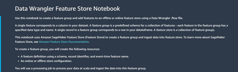
Choose Export step and Feature Store to automatically create your notebook. This notebook recreates the manual steps you created, creates a feature group, and adds features to an offline or online feature store, allowing you easily rerun your manual steps.

This notebook defines the schema instead of auto-detection of data types for each column of the data, with the following format:

column_schema = [
 { 
 "name": "Height", 
 "type": "long" 
 },
 { 
 "name": "Sum", 
 "type": "string" 
 }, 
 { 
 "name": "Time", 
 "type": "string"
  }
]

For more information on how to load the schema, map it, and add it as a FeatureDefinition that you can use to create the FeatureGroup, see Export to the SageMaker Feature Store.

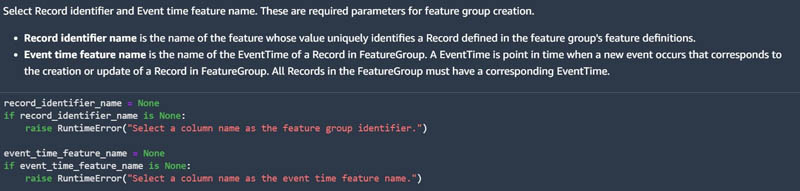
Additionally, you must specify a record identifier name and event time feature name in the following code:

  • The record_identifier_name is the name of the feature whose value uniquely identifies a record defined in the feature store.
  • An EventTime is a point in time when a new event occurs that corresponds to the creation or update of a record in a feature. All records in the feature group must have a corresponding EventTime.

The notebook creates an offline store and the online by default with the following configuration set to True:

online_store_config = {
    "EnableOnlineStore": True
}

You can also disable an online store by setting EnableOnlineStore to False in the online and offline store configurations.

You can then run the notebook, and the notebook creates a feature group and processing job to process data in scale. The offline store is located in an Amazon Simple Storage Service (Amazon S3) bucket in your AWS account. Because Feature Store is integrated with Amazon SageMaker Studio, you can visualize the feature store by choosing Components and registries in the navigation pane, choosing Feature Store on the drop-down menu, and then finding your feature store on the list. You can check for feature definitions, manage feature group tags, and generate queries for the offline store.

Build a training set from an offline store

Now that you have created a feature store from your processed data, you can build a training dataset from your offline store by using services such as Amazon Athena, AWS Glue, or Amazon EMR. In the following example, because Feature Store automatically builds an AWS Glue Data Catalog when you create feature groups, you can easily create a training dataset with feature values from the feature group. This is done by utilizing the auto-built Data Catalog.

First, create an Athena query for your feature group with the following code. The table_name is the AWS Glue table that is automatically generated by Feature Store.

sample_query = your_feature_group.athena_query()
data_table = sample_query.table_name

You can then write your query using SQL on your feature group, and run the query with the .run() command and specify your S3 bucket location for the dataset to be saved there. You can modify the query to include any operations needed for your data like joining, filtering, ordering, and so on. You can further process the output DataFrame until it’s ready for modeling, then upload it to your S3 bucket so that your SageMaker trainer can directly read the input from the S3 bucket.

# define your Athena query
query_string = 'SELECT * FROM "'+data_table+'"'

# run Athena query. The output is loaded to a Pandas dataframe.
dataset = pd.DataFrame()
sample_query.run(query_string=query_string, output_location='s3://'+default_s3_bucket_name+'/query_results/')
sample_query.wait()
dataset = sample_query.as_dataframe()

Access your Feature Store for inference

After you build a model from the training set, you can access your online store conveniently to fetch a record and make predictions using the deployed model. Feature Store can be especially useful in supplementing data for inference requests because of the low-latency GetRecord functionality. In this example, you can use the following code to query the online feature group to build an inference request:

selected_id = str(194)

# Helper to parse the feature value from the record.

def get_feature_value(record, feature_name):
    return str(list(filter(lambda r: r['FeatureName'] == feature_name, record))[0]['ValueAsString'])

fs_response = featurestore_runtime.get_record(
                                               FeatureGroupName=your_feature_group_name,
                                               RecordIdentifierValueAsString=selected_id)
selected_record = fs_response['Record']
inference_request = [
    get_feature_value(selected_record, 'feature1'),
    get_feature_value(selected_record, 'feature2'),
    ....
    get_feature_value(selected_record, 'feature 10')
]

You can then call the deployed model predictor to generate a prediction for the selected record:

results = predictor.predict(','.join(inference_request), 
                            initial_args = {"ContentType": "text/csv"})
prediction = json.loads(results)

Integrate Feature Store in a SageMaker pipeline

Feature Store also integrates with Amazon SageMaker Pipelines to create, add feature search and discovery to, and reuse automated ML workflows. As a result, it’s easy to add feature search, discovery, and reuse to your ML workflow. The following code shows you how to configure the ProcessingOutput to directly write the output to your feature group instead of Amazon S3, so that you can maintain your model features in a feature store:

flow_step_outputs = []
flow_output = sagemaker.processing.ProcessingOutput(
    output_name=customers_output_name,
    feature_store_output=sagemaker.processing.FeatureStoreOutput(
        feature_group_name=your_feature_group_name), 
    app_managed=True)
flow_step_outputs.append(flow_output)

example_flow_step = ProcessingStep(
    name='SampleProcessingStep', 
    processor=flow_processor, # Your flow processor defined at the beginning of your pipeline
    inputs=flow_step_inputs, # Your processing and feature engineering steps, can be Data Wrangler flows
    outputs=flow_step_outputs)

Conclusion

In this post, we explored how Feature Store can be a powerful tool in your ML journey. You can easily export your data processing and feature engineering results to a feature group and build your feature store. After your feature store is all set up, you can explore and build training sets from your offline store, taking advantage of its integration with other AWS analytics services such as Athena, AWS Glue, and Amazon EMR. After you train and deploy a model, you can fetch records from your online store for real-time inference. Lastly, you can add a feature store as a part of a complete SageMaker pipeline in your ML workflow. Feature Store makes it easy to store and retrieve features as needed in ML development.

Give it a try, and let us know what you think!


About the Author

As a data scientist and consultant, Zoe Ma has helped bring the latest tools and technologies and data-driven insights to businesses and enterprises. In her free time, she loves painting and crafting and enjoys all water sports.

Courtney McKay is a consultant. She is passionate about helping customers drive measurable ROI with AI/ML tools and technologies. In her free time, she enjoys camping, hiking and gardening.

Read More