Partnering with the NSF on a research institute for AI to improve care for older adults

From the early days of the internet to the development of the Human Genome Project, U.S. government-funded R&D has yielded remarkable progress for society, and today it is an important engine for AI research. That’s why, last year, we were proud to announce our partnership with the U.S. National Science Foundation (NSF) to provide $5M to support the establishment of national research institutes working in the area of Human-AI Interaction and Collaboration (HAIC). This partnership—which is part of a more than $300M NSF investment in AI Research Institutes—will create vibrant research centers across the U.S. to advance how people and AI collaborate through speech, text, gestures, and more. It also builds on our partnership with the NSF on next generation networks, and our AI research collaborations with U.S. federal agencies on weather modeling, robust AI systems, whale population monitoring, and more. 

Today, we are delighted to share that NSF has selected the AI Institute for Collaborative Assistance and Responsive Interaction for Networked Groups (AI-CARING) led by Georgia Tech, along with Carnegie Mellon University, Oregon State University, and University of Massachusetts Lowell to receive the $20M AI Institute for HAIC grant. AI-CARING will improve collaboration and communication in caregiving environments for older adults by developing AI systems that adjust to the evolving personal needs and behaviors of those requiring care. With our growing research presence in Atlanta, we’re excited to build on our rich history of collaboration with Georgia Tech and its partners in this effort—most recently supporting some of these universities’ work to help vulnerable populations find important information on COVID-19 and monitoring and forecasting disease spread.

With a growing population of older adults in need of caregiving, AI systems can be useful in a variety of contexts, like conversational assistants, health sensing, and improving coordination across the care network. For example, AI can help existing voice assistants better understand people with speech impairments, and can be integrated in home bathrooms to make them more accessible. The AI-CARING Institute will develop assistive AI agents across these types of contexts to help those requiring caregiving to sustain their independence and  improve their quality of life. Additionally, this research will be the product of interdisciplinary teams—with expertise across AI, geriatrics, behavioral sciences, and design—working to ensure that AI is deployed responsibly in this context, with human-centered principles in mind.

Congratulations to the recipient universities of the AI Institute awards and the faculty, listed below. We look forward to learning from the team’s research, sharing our resources and expertise, and building a collaboration to help older adults lead more independent lives and improve the quality of their care.

Recipient university institutions:

  • Georgia Institute of Technology
  • Carnegie Mellon University
  • Oregon State University
  • University of Massachusetts Lowell

Faculty:

  • Sonia Chernova (Georgia Tech) – PI
  • Elizabeth Mynatt (Georgia Tech) – Co-PI
  • Reid Simmons (Carnegie Mellon University) – Co-PI
  • Kagan Tumer (Oregon State University) – Co-PI
  • Holly Yanco (University of Massachusetts Lowell) – Co-PI

Read More

GFN Thursday Brings ‘Evil Genius 2: World Domination,’ ‘Escape From Naraka’ with RTX, and More This Week on GeForce NOW

This GFN Thursday shines a spotlight on the latest games joining the collection of over 1,000 titles in the GeForce NOW library from the many publishers that have opted in to stream their games on our open cloud-gaming service.

Members can look forward to 14 games — including Evil Genius 2: World Domination from Rebellion and Escape From Naraka, which features RTX for Founders and Priority members — joining the GeForce NOW library this week. Team17’s Hell Let Loose, already streaming on GeForce NOW, has left early access with the introduction of the Soviet forces on the eastern front.

Getting Rebellious

Ready to take over the world? This GFN Thursday, stream several exciting titles from Rebellion — the award-winning British independent studio. Games include Evil Genius 2: World Domination, Evil Genius, Battlezone: Combat Commander and Zombie Army 4: Dead War.

Evil Genius 2 on GeForce NOW
Become a criminal mastermind in this wicked awesome sequel.

Be the best bad guy you can be in Evil Genius 2: World Domination (Steam). Construct an evil lair, train your minions to carry out nefarious plans and fight against the Forces of Justice with an array of traps to achieve global domination in this satirical spy-fi lair-builder game.

Members can also look forward to the original Evil Genius coming to the cloud this week, as well as Battlezone: Combat Commander for space-shooting intergalactic battles. And gamers can sink their teeth into Zombie Army 4: Dead War for the fight against the undead Armageddon. With all of these new additions, more gamers now can play these awesome titles from Rebellion.

“GeForce NOW gives us a great opportunity to provide access to our catalog of games to even more gamers,” said Matt Jeffery, chief strategy officer at Rebellion. “NVIDIA makes onboarding games to the cloud a simple process, helping us bring our games to players on low-powered or incompatible devices, with the power of a real gaming rig.”

These newest additions join a host of other Rebellion titles available to stream on GeForce NOW, including Sniper Elite 3, Sniper Elite 4 and Sniper Elite V2 Remastered for players who aim to have a good time with a stealth story. Plus more undead action in the Zombie Army Trilogy and an adventure full of puzzles, traps and mummies in Strange Brigade that’s too good to keep under wraps.

Heating Things Up

The front line is calling. Hell Let Loose (Steam) from Team17 has left early access and is streaming in open access on GeForce NOW.

Charge into battle in this hardcore World War II first-person shooter with epic battles and players filling roles of infantry, tanks, artillery and the dynamically shifting front line. Battle across more than nine maps modeled on real-life locales. Fight in iconic battles from the Western Front, including Carentan, Omaha Beach, Foy and more. Members can experience the chaos of all-out war and stream Hell Let Loose with GeForce NOW this week.

Members can also check out other popular titles from Team17 in the GeForce NOW library, including multiplayer games like Overcooked! and Overcooked! 2 and Golf with Friends for gamers looking to play with friends. Or experience a variety of RPGs with the cozy and creative Hokko Life, the pirate adventure King of the Seas, and the alien world of Planet Alpha.

Up This Week

As always, GFN Thursday means more games. This week, members can journey to a nightmarish temple in Escape from Naraka and save their beloved from an evil demon of legend.

Escape from Naraka on GeForce NOW
Don’t miss out on a new adventure with ‘Escape from Naraka,’ one of 14 titles joining GeForce NOW this week.

Complete challenges, unlock the secrets of the temple and use unique abilities to confront terrifying enemies and escape the temple. Founders and Priority members can play Escape from Naraka on GeForce NOW with beautifully ray-traced reflections, ray-traced shadows and RTX Global Illumination.

Here’s the complete list of 14 titles coming to the cloud this week:

And while you decide which of these games to spend your weekend with, we have an important question for you.

who’s the most iconic villain in video game history? 🤔

🌩 NVIDIA GeForce NOW (@NVIDIAGFN) July 28, 2021

Shout it out on Twitter, and we’ll see you next week!

The post GFN Thursday Brings ‘Evil Genius 2: World Domination,’ ‘Escape From Naraka’ with RTX, and More This Week on GeForce NOW appeared first on The Official NVIDIA Blog.

Read More

Facebook Fellow Spotlight: Empowering women in rural communities through research in HCI

Each year, PhD students from around the world apply for the Facebook Fellowship, a program designed to encourage and support doctoral students engaged in innovative and relevant research in areas related to computer science and engineering at an accredited university.

As a continuation of our Fellowship spotlight series, we’re highlighting 2020 Facebook Fellow Sharifa Sultana.

Sharifa is a PhD candidate in Information Science at Cornell University. Her work focuses on human-computer interaction (HCI) and information and communication technologies for development (ICTD) from a critical computing and feminist HCI perspective.

Raised in Jessore, Bangladesh, Sharifa noticed that women were underrepresented in STEM education and other professions around the world, particularly in Bangladesh. Because of this underrepresentation, many women in rural communities have difficulties accessing, trusting, and using technology. This inspired Sharifa to work towards creating a more inclusive environment in which women would feel empowered to use technology, and where technology could, in turn, help fight the oppression of women in her home country.

“My research asks the questions, ‘Why is tech not working for rural Bangladeshi women? How can we fight against oppression using tech?’” she says. Sharifa’s approach explores how women interact with technology in rural communities in an effort to develop and implement solutions that address their critical needs.

One of these needs is combating gender harassment. “In Bangladesh, women are often harassed by colleagues, friends, family members — people who they want to trust,” she says. “Yet it is often difficult for them to seek legal help for many reasons.”

In order to empower women to counter harassment, Sharifa designed a digital tool – ‘Unmochon’ – to collect evidence of tech-based harassment through Facebook Messenger. Users can install and run it to collect image evidence of harassing messages and the harassers’ Facebook handles. This tool allows users to report the incident to the appropriate authorities and confirm the authenticity of the evidence.

Sharifa’s most recent research focuses on alternative rationalities in computing – namely, exploring how rural communities determine what information is true and how misinformation can prevent women from seeking healthcare. “The aim is to design tech that would actually help [women], that they would actually use,” Sharifa says.

Healthcare misinformation is a serious issue for rural communities in Bangladesh, especially during the COVID-19 pandemic. She hopes to develop technology that will give people access to reliable information and connect them with the healthcare they need.

Sharifa’s research has opened up a new discussion on how HCI design can be used to address online gender harassment and on how studying HCI can help bridge the gap between women accessing life-saving healthcare. Currently, Sharifa is in Bangladesh, collaborating on a local research project to determine what kind of technology and healthcare practices could benefit rural communities.

To learn more about Sharifa Sultana, visit her Fellowship profile.

The post Facebook Fellow Spotlight: Empowering women in rural communities through research in HCI appeared first on Facebook Research.

Read More

Orchestrate XGBoost ML Pipelines with Amazon Managed Workflows for Apache Airflow

The ability to scale machine learning operations (MLOps) at an enterprise is quickly becoming a competitive advantage in the modern economy. When firms started dabbling in ML, only the highest priority use cases were the focus. Businesses are now demanding more from ML practitioners: more intelligent features, delivered faster, and continually maintained over time. An effective MLOps strategy requires a unified platform that can orchestrate and automate complex data processing and ML tasks, and integrates with the latest tooling to best complete those tasks.

This post demonstrates the value of using Amazon Managed Workflows for Apache Airflow (Amazon MWAA) to orchestrate an ML pipeline using the popular XGBoost (eXtreme Gradient Boosting) algorithm. For more advanced and comprehensive MLOps capabilities, including a purpose-built model orchestration framework and a continuous integration and continuous delivery (CI/CD) service for ML, readers are encouraged to check out Amazon SageMaker Pipelines.

Why Airflow for orchestration

Customers choose Apache Airflow and specifically Amazon MWAA for several reasons, but three stand out:

  • Airflow is Python-based – Airflow, as a Python-based tool, enjoys the benefits of an imperative programming paradigm. This enables developers to programmatically define how tasks are to be done. Tools that are declarative, such as AWS Step Functions, only allow you to define what is to be done. When orchestrating ML pipelines, the ability to directly define the control flow is often required to navigate complex workflows.
  • Directed Acyclic Graph (DAG) workflow management – Airflow provides a DAG interface as a simple mechanism for defining and running complex workflows with dependencies. These DAG workflows are visualized through a GUI for operations management.
  • Extensibility – Airflow operators provide a structured way to perform common tasks using reusable modules. This capability is extensible and providers are free to develop custom Airflow operators that integrate with their tools and services. Many cloud-based services are supported. These operators provide useful abstraction, repeatability, and an API. In the context of big data and ML, these operators are especially valuable because they provide a way to orchestrate sometimes very long-running data pipelines or asynchronous ML processes such as model training.

Set up an Amazon MWAA environment

To create your Amazon MWAA environment, complete the following steps:

  1. On the Amazon MWAA console, choose Create environment.
  2. For Name, enter a unique name.
  3. For Airflow version, choose the version to use. For this post, we use Airflow v2.0.2. We also include code for Airflow v1.10.12.

  1. In the Dag code in the Amazon S3 section, specify the Amazon Simple Storage Service (Amazon S3) bucket where Amazon MWAA can find the DAGs, plugins.zip file, and requirements.txt file.

Airflow configuration for XGBoost

An XGBoost model requires a specific configuration in the Managed Airflow environment. The core.enable_xcom_pickling parameter must be set to True. The reason for this is the trained XGBoost model needs to be serialized in order to save it as a file in Amazon S3. Certain Python objects (like datetime) can’t be serialized without converting the Python object hierarchy into a byte stream through a process called pickling.

Requirements.txt file

Upload a requirements.txt file to the Amazon S3 location you specified in the Amazon MWAA setup. To support this demonstration, the requirements.txt file should have the following entries:

boto3==1.17.49
sagemaker==1.72.0
s3fs==0.5.1

Orchestrate an XGBoost ML pipeline

Our ML pipeline is a simplified three-step pipeline:

  1. Data preprocessing using AWS Glue. Real pipelines could require numerous processing steps for data cleaning and featuring engineering. Although Amazon SageMaker Pipelines provides a similar functionality, we use AWS Glue to illustrate how different AWS services or third-party tools and services are orchestrated in a single pipeline.
  2. Train an XGBoost model using a SageMaker training job.
  3. Deploy the trained model as a real-time inference endpoint.

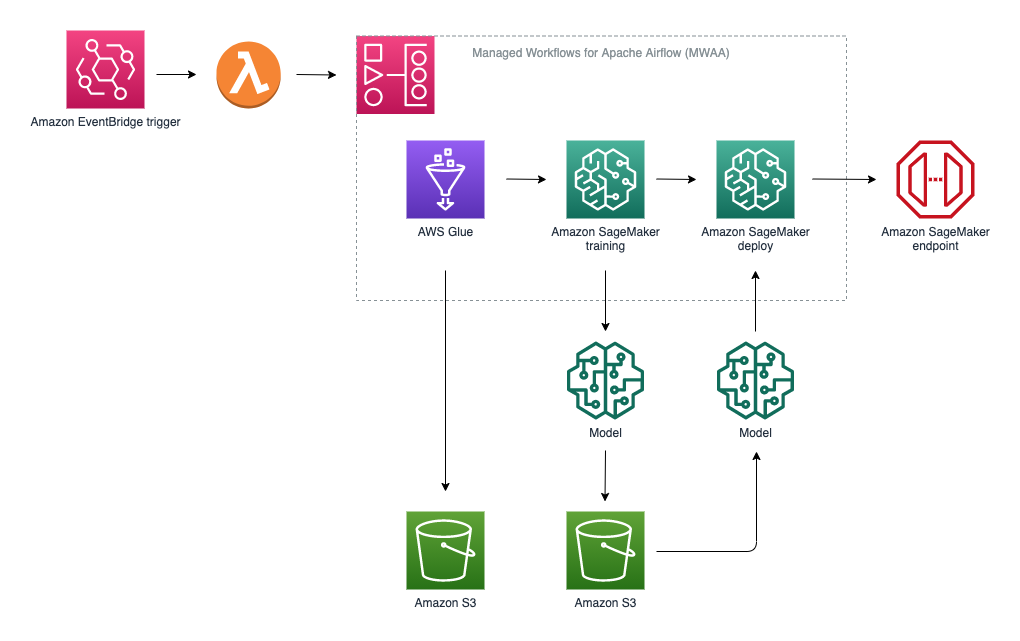
Solution architecture

Our ML pipeline is pictured in the following diagram. We use AWS Lambda to invoke DAGs with a Lambda function. We also use Amazon EventBridge to trigger Lambda functions. For more information, see Tutorial: Schedule AWS Lambda functions using EventBridge.

Stage the AWS Glue script

In our demo, we create the AWS Glue job dynamically using a PySpark script saved in Amazon S3. Copy the glue_etl.py file provided in the source code repo to an Amazon S3 location.

Set DAG configuration values

To keep things simple, we use a config.py file to import any environment-specific configurations rather than define it in the main DAG script. You can view the config.py file in its entirety on GitHub. A best practice is to use AWS Secrets Manager to store configuration and secrets information (as of this writing, AWS Systems Manager Parameter Store isn’t a supported backend on Amazon MWAA). Detailed documentation on how to securely store secrets in AWS Secrets Manager for Amazon MWAA is available here.

Upload the updated config.py file to the DAG directory.

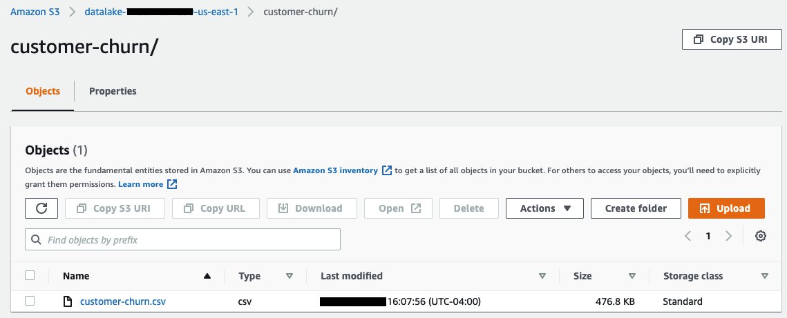
Stage the customer churn training data

The customer churn dataset is mentioned in the book Discovering Knowledge in Data by Daniel T. Larose. It’s attributed by the author to the University of California Irvine Repository of Machine Learning Datasets. The dataset is publicly available and provided in the GitHub repo.

Upload the customer-churn.csv file to the Amazon S3 location you specified in the config.py file.

Construct the DAG

For our demonstration, the DAG consists of four primary sections:

  • Import statements
  • DAG operator configuration
  • DAG task definitions
  • DAG task dependency definition

Import statements

Because Airflow is Python-based, the DAG file is a simple Python file and the modules for Airflow are imported just as they would be for any Python application.

Some services have native Airflow operators available that manage asynchronous API calls and polling to determine success or failure of orchestrated tasks. We recommend using native operators wherever possible. AWS services that don’t have native Airflow operators, like AWS Glue, can still be orchestrated in Airflow using AWS SDKs called from the general PythonOperator.

For nearly all AWS services, the AWS SDK for Python (Boto3) provides service-level access to the APIs. This SDK provides a high degree of control, but also a lower level of abstraction. For ML pipelines using SageMaker, you can use the SageMaker Python SDK. This is a streamlined SDK abstracted specifically for ML experimentation.

The following import statements include general Airflow modules and operators, native Airflow operators for SageMaker, and the Boto3 and SageMaker SDKs:

# Airflow Operators
import airflow
from airflow.models import DAG
from airflow.utils.dates import days_ago
from airflow.operators.python_operator import PythonOperator

# Airflow Sagemaker Operators
from airflow.providers.amazon.aws.operators.sagemaker_training import SageMakerTrainingOperator
from airflow.providers.amazon.aws.operators.sagemaker_endpoint import SageMakerEndpointOperator
from airflow.providers.amazon.aws.hooks.base_aws import AwsBaseHook

# AWS SDK for Python
import boto3

# Amazon SageMaker SDK
import sagemaker
from sagemaker.amazon.amazon_estimator import get_image_uri
from sagemaker.estimator import Estimator
from sagemaker.session import s3_input

# Airflow SageMaker Configuration
from sagemaker.workflow.airflow import training_config
from sagemaker.workflow.airflow import model_config_from_estimator
from sagemaker.workflow.airflow import deploy_config_from_estimator

# Configuration variables
import config

Other import statements are needed to support this demonstration; refer to the GitHub repo for the full code.

DAG operator configuration

The DAG and DAG tasks are defined based on the operators invoked to run each task.

For the AWS Glue task, we invoke the PythonOperator using the SDK for Python to create a client for AWS Glue. To keep the DAG code tidy, we abstract the AWS Glue client code in a helper function called preprocess_glue. We stage the glue_etl.py (referenced in the GitHub repo) in Amazon S3 so it can be loaded when the AWS Glue job is created. See the following code:

def preprocess_glue():
  """preprocess data using glue for etl"""

  # not best practice to hard code location 
  glue_script_location = 's3://{}/{}'.format(config.GLUE_JOB_SCRIPT_S3_BUCKET, config.GLUE_JOB_SCRIPT_S3_KEY)
  glue_client = boto3.client('glue')

  # instantiate the Glue ETL job
  response = glue_client.create_job(
    Name=glue_job_name,
    Description='PySpark job to extract the data and split in to training and validation data sets',
    Role=config.GLUE_ROLE_NAME,
    ExecutionProperty={
      'MaxConcurrentRuns': 2
    },
    Command={
      'Name': 'glueetl',
      'ScriptLocation': glue_script_location,
      'PythonVersion': '3'
    },
    DefaultArguments={
      '--job-language': 'python'
    },
    GlueVersion='1.0',
    WorkerType='Standard',
    NumberOfWorkers=2,
    Timeout=60
    )
  
  # execute the previously instantiated Glue ETL job
  response = glue_client.start_job_run(
    JobName=response['Name'],
    Arguments={
      '--S3_SOURCE': config.DATA_S3_SOURCE,
      '--S3_DEST': config.DATA_S3_DEST,
      '--TRAIN_KEY': 'train/',
      '--VAL_KEY': 'validation/' 
    }
  )

We create a helper function that returns the ARN of the SageMaker role:

def get_sagemaker_role_arn(role_name, region_name):
    iam = boto3.client("iam", region_name=region_name)
    response = iam.get_role(RoleName=role_name)
    return response["Role"]["Arn"]

The XGBoost estimator requires the SageMaker role, container image, and hyperparameters, which we collect using a hook into SageMaker:

hook = AwsBaseHook(aws_conn_id="airflow-sagemaker", client_type="sagemaker")
sess = hook.get_session(region_name=config.REGION_NAME)
sagemaker_role = get_sagemaker_role_arn(config.SAGEMAKER_ROLE_NAME, config.REGION_NAME)
container = get_image_uri(sess.region_name, "xgboost")
hyperparameters = {
    "max_depth":"5",
    "eta":"0.2",
    "gamma":"4",
    "min_child_weight":"6",
    "subsample":"0.8",
    "objective":"binary:logistic",
    "num_round":"100"
}

With the parameters defined, we can create the estimator object:

xgb_estimator = Estimator(
    image_name=container, 
    hyperparameters=hyperparameters,
    role=sagemaker_role,
    sagemaker_session=sagemaker.session.Session(sess),
    train_instance_count=1, 
    train_instance_type='ml.m5.4xlarge', 
    train_volume_size=5,
    output_path=config.SAGEMAKER_MODEL_S3_DEST
)

This estimator object is an input parameter into the training configuration. We need to define other training parameters:

# create unique name with guid
sagemaker_taining_job_name=config.SAGEMAKER_TRAINING_JOB_NAME_PREFIX+'-{}'.format(guid)

# define S3 locations for training & validation data processed using Glue
sagemaker_training_data = s3_input(config.SAGEMAKER_TRAINING_DATA_S3_SOURCE, content_type=config.SAGEMAKER_CONTENT_TYPE)
sagemaker_validation_data = s3_input(config.SAGEMAKER_VALIDATION_DATA_S3_SOURCE, content_type=config.SAGEMAKER_CONTENT_TYPE)

sagemaker_training_inputs = {
  'train': sagemaker_training_data,
  'validation': sagemaker_validation_data
  }

Let’s take a closer look at the arguments for sagemaker_training_inputs. The XGBoost algorithm supports both LIBSVM and CSV text formats for training and validation datasets. However, LIBSVM is supported by default. This means that we must specify CSV explicitly so XGBoost interprets our data correctly. The content type is set as text/csv in our custom DAG configuration file. We use CSV because it’s the most common data file format familiar to all ML practitioners.

With these parameters defined, we can create the training config object:

training_config = training_config(
  estimator=xgb_estimator,
  inputs=sagemaker_training_inputs,
  job_name=sagemaker_taining_job_name
)

For native Airflow SageMaker operators, you can construct and reference well-defined configuration objects when invoking the operators.

The next configuration definition is for the SageMaker endpoint:

# create unique name using guid
sagemaker_model_name=config.SAGEMAKER_MODEL_NAME_PREFIX+'-{}'.format(guid)
sagemaker_endpoint_name=config.SAGEMAKER_ENDPOINT_NAME_PREFIX+'-{}'.format(guid)

For this simple pipeline, we use the deploy_config_from_estimator API option in the SageMaker SDK to export an Airflow deploy config directly from the SageMaker XGBoost estimator (the endpoint_name parameter must be 63 characters or less):

endpoint_config = deploy_config_from_estimator(
  estimator=xgb_estimator, 
  task_id="train", 
  task_type="training", 
  initial_instance_count=1, 
  instance_type="ml.m4.xlarge",
  model_name=sagemaker_model_name,
  endpoint_name=sagemaker_endpoint_name
)

For more information about how we set up the model training and deployment configuration, including how we used the SageMaker SDK sagemaker.workflow.airflow APIs, see the GitHub repo.

With the operator configuration complete, we’re ready to put it all together to define our DAG.

DAG task definitions

For the XGBoost model training task, we invoke the SageMakerTrainingOperator. For the endpoint deployment task, we invoke the SageMakerEndpointOperator. It’s important to note the separation of concerns: we create a model using the SageMakerModelOperator but configure the SageMaker endpoint using the SageMakerEndpointConfigOperator. This provides added granular control over the creation and deployment of the model. See the following code:

args = {"owner": "airflow", "start_date": airflow.utils.dates.days_ago(2), 'depends_on_past': False}

with DAG(
    dag_id=config.AIRFLOW_DAG_ID,
    default_args=args,
    start_date=days_ago(2),
    schedule_interval=None,
    concurrency=1,
    max_active_runs=1,
) as dag:
    process_task = PythonOperator(
      task_id="process",
      dag=dag,
      #provide_context=False,
      python_callable=preprocess_glue,
    )

    train_task = SageMakerTrainingOperator(
      task_id = "train",
      config = training_config,
      aws_conn_id = "airflow-sagemaker",
      wait_for_completion = True,
      check_interval = 60, #check status of the job every minute
      max_ingestion_time = None, #allow training job to run as long as it needs, change for early stop
    )

    endpoint_deploy_task = SageMakerEndpointOperator(
      task_id = "endpoint-deploy",
      config = endpoint_config,
      aws_conn_id = "sagemaker-airflow",
      wait_for_completion = True,
      check_interval = 60, #check status of endpoint deployment every minute
      max_ingestion_time = None,
      operation = 'create', #change to update if you are updating rather than creating an endpoint
    )

DAG task dependency definition

After we define the tasks, we set the dependencies of the tasks. Airflow implements the right shift logical operator (>>) to define downstream dependencies and the left shift logical operator (<<) to define upstream dependencies. In our example, we only define downstream dependencies:

# set the dependencies between tasks
process_task >> train_task >> endpoint_deploy_task

When the completed DAG is uploaded to the designated Amazon S3 location, Amazon MWAA automatically ingests the DAG. The graph view visually shows the task dependencies. You can trigger the DAG manually from the console during iterative testing, or as we described earlier, from an external source such as EventBridge and a Lambda function. Each task is highlighted depending on the stage of completion, as shown in the following screenshot. Dark green indicates successful completion of the task.

Test the deployed endpoint

After the endpoint-deploy task is complete, we can view the endpoint on the SageMaker console. The SageMaker endpoint is a real-time inference endpoint. SageMaker takes care of deploying, hosting, and exposing the HTTPS endpoint.

We can test the deployed endpoint with a SageMaker notebook.

Follow these steps to set up a SageMaker notebook environment:

  1. Launch a SageMaker notebook instance.
  2. On the Notebook instances page, open your notebook instance by choosing either Open JupyterLab for the JupyterLab interface or Open Jupyter for the classic Jupyter view.
  3. Choose Upload to import the test notebook available in the GitHub repo.

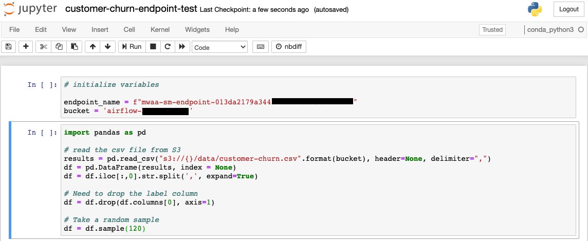
Prepare a test sample

We use Pandas DataFrames to create a test dataset out of the customer churn dataset that was used for training. For the test dataset, we must drop the label column, which is the first column. We also take a random sample of the dataset using the Pandas DataFrame sample method.
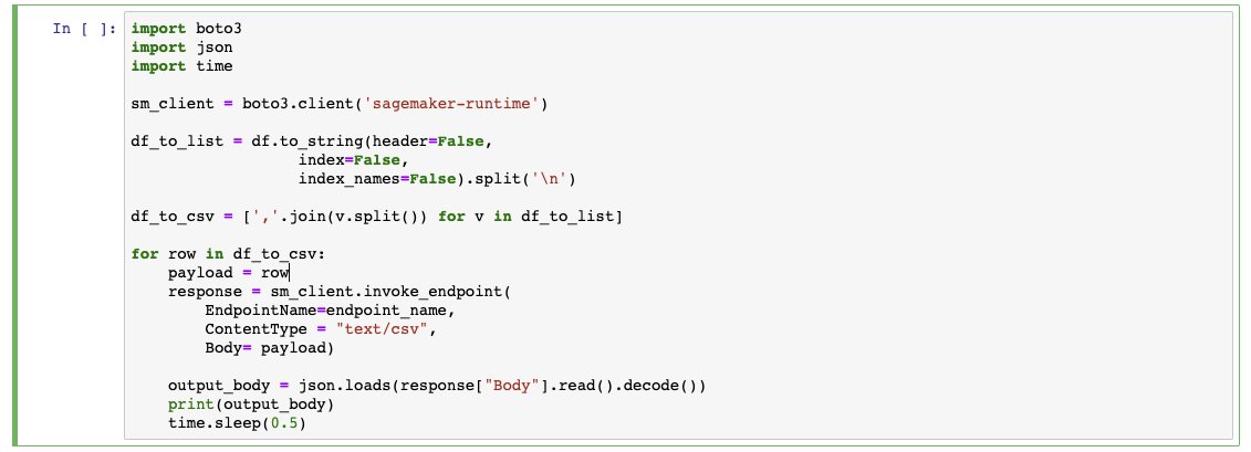
Request inferences

Now that we have our sampled test data, we use the Boto3 library to create a SageMaker runtime client. We use the client when we invoke our endpoint, pass it test data, and receive an inference value.

Conclusion

You can use Amazon MWAA to orchestrate and automate complex ML pipelines from the data processing stage through model training and endpoint deployment. You can set special configuration options in the Amazon MWAA environment to support popular ML frameworks like XGBoost.

In this post, we demonstrated how to dynamically create and run an AWS Glue job to preprocess training and validation data. We showed how to construct the DAG to support this ML pipeline, including the import statements, the DAG operator configuration, the DAG task definitions, and the DAG dependency definition. We demonstrated the difference between using native Airflow operators vs. invoking AWS SDK API calls from a generic PythonOperator.

Amazon MWAA is a highly versatile orchestration tool that enterprises can use to operationalize and scale their ML capabilities.


About the authors

Justin Leto is a Sr. Solutions Architect at Amazon Web Services with specialization in big data analytics and machine learning. His passion is helping customers achieve better cloud adoption. In his spare time, he enjoys offshore sailing and playing jazz piano. He lives in Manhattan with his wife Veera.


David Ehrlich is a Machine Learning Specialist at Amazon Web Services. He is passionate about helping customers unlock the true potential of their data. In his spare time, he enjoys exploring the different neighborhoods in New York City, going to comedy clubs, and traveling.


Shreyas Subramanian is a AI/ML specialist Solutions Architect, and helps customers by using Machine Learning to solve their business challenges using AWS services.

Read More

Using AI to map Africa’s buildings

Between 2020 and 2050, Africa’s population is expected to double, adding 950 million more people to its urban areas alone. However, according to 2018 figures, a scarcity of affordable housing in many African cities has forced over half of the city dwellers in Sub-Saharan Africa to live in informal settlements. And in rural areas, many also occupy makeshift structures due to widespread poverty.

These shelters have remained largely undetectable using traditional monitoring tools. Machine learning, computer vision and remote sensing have come some way in recognizing buildings and roads, but when it comes to denser neighborhoods, it becomes much harder to distinguish small and makeshift buildings. 

Why is this an issue? Because when preparing a humanitarian response, forecasting transportation needs, or planning basic services, being able to accurately map the built environment – which allows us to ascertain population density – is absolutely key.

Enter Google’s Open Buildings

Google’s Open Buildings is a new open access dataset containing the locations and geometry of buildings across most of Africa. From Lagos’ Makoko settlement to Dadaab’s refugee camps, millions of previously invisible buildings have popped up in our dataset. This improved building data helps refine the understanding of where people and communities live, providing actionable information for state and non-state actors looking to provide services from sanitation to education and vaccination.

  • An aerial photograph of a refugee settlement in Uganda

    Refugee settlement in Yumbe district, Uganda

  • An aerial photograph of rural dwellings in Ethiopia

    Rural dwellings in Sholtaka, Ethiopia

  • An aerial photograph of an urban area in DRC

    High density urban area in Kinshasa, DRC

Open Buildings uses AI to provide a digital footprint of buildings. This includes producing polygons with the outlines of at least 500 million buildings across the African continent, the majority of which are less than 20 square meters. The full dataset encompasses 50 countries.

The data provides the exact location and polygon outline of each building, its size, a confidence score for it being detected as a valid building and a Plus Code. There is, however, no information about the type of building, its street address, or any identifying data. We have also excluded sensitive areas such as conflict zones to protect vulnerable populations.

Satellite mapping using AI 

The Open Buildings dataset was generated by using a model trained to detect buildings using satellite imagery from the African continent. The information for the buildings detected is then saved in CSV files which are available to download. The technical details of the Open Buildings dataset, including usage and tutorials, are available on the dataset website and the Google AI blog.

Animation showing landscape in Africa being mapped

How will this improve planning?

There are many important ways in which this data can be used, including — but not limited to — the following:

Population mapping: Building footprints are a key ingredient for estimating population density. This information is vital to planning for services for communities. 

Humanitarian response: To plan the response to a flood, drought, or other natural disaster.

Environmental science: Knowledge of settlement density is useful for understanding the human impact on the natural environment. 

Addressing systems: In many areas, buildings do not have formal addresses. This can make it difficult for people to access social benefits and economic opportunities. Building footprint data can help with the rollout of digital addressing systems such asPlus Codes.

Vaccination planning: Knowing the density of population and settlements helps to anticipate demand for vaccines and the best locations for facilities. This data is also useful for precision epidemiology, as well as prevention efforts such as mosquito net distribution.

Statistical indicators: Buildings data can be used to help calculate statistical indicators for national planning, such as the numbers of houses in the catchment areas of schools and health centers, mean travel distances to the nearest hospital or demand forecast for transportation systems.

Google’s AI Center in Accra

This project was led by our team at the AI Research Center in Accra, Ghana. The center was launched in 2019 to bring together top machine learning researchers and engineers dedicated to AI research and its applications. The research team has already been improving Google Maps with AI, adding 120 million buildings and 228,000 km of roads across Africa to Maps in the last year. This work is part of our broader AI for Social Good efforts.

Read More

Introducing Triton: Open-Source GPU Programming for Neural Networks

Introducing Triton: Open-Source GPU Programming for Neural Networks

We’re releasing Triton 1.0, an open-source Python-like programming language which enables researchers with no CUDA experience to write highly efficient GPU code—most of the time on par with what an expert would be able to produce. Triton makes it possible to reach peak hardware performance with relatively little effort; for example, it can be used to write FP16 matrix multiplication kernels that match the performance of cuBLAS—something that many GPU programmers can’t do—in under 25 lines of code. Our researchers have already used it to produce kernels that are up to 2x more efficient than equivalent Torch implementations, and we’re excited to work with the community to make GPU programming more accessible to everyone.


Novel research ideas in the field of Deep Learning are generally implemented using a combination of native framework operators. While convenient, this approach often requires the creation (and/or movement) of many temporary tensors, which can hurt the performance of neural networks at scale. These issues can be mitigated by writing specialized GPU kernels, but doing so can be surprisingly difficult due to the many intricacies of GPU programming. And, although a variety of systems have recently emerged to make this process easier, we have found them to be either too verbose, lack flexibility or generate code noticeably slower than our hand-tuned baselines. This has led us to extend and improve Triton, a recent language and compiler whose original creator now works at OpenAI.

The Challenges of GPU Programming

The architecture of modern GPUs can be roughly divided into three major components—DRAM, SRAM and ALUs—each of which must be considered when optimizing CUDA code:

  • Memory transfers from DRAM must be coalesced into large transactions to leverage the large bus width of modern memory interfaces.
  • Data must be manually stashed to SRAM prior to being re-used, and managed so as to minimize shared memory bank conflicts upon retrieval.
  • Computations must be partitioned and scheduled carefully, both across and within Streaming Multiprocessors (SMs), so as to promote instruction/thread-level parallelism and leverage special-purpose ALUs (e.g., tensor cores).
Introducing Triton: Open-Source GPU Programming for Neural Networks
Basic architecture of a GPU.

Reasoning about all these factors can be challenging, even for seasoned CUDA programmers with many years of experience. The purpose of Triton is to fully automate these optimizations, so that developers can better focus on the high-level logic of their parallel code. Triton aims to be broadly applicable, and therefore does not automatically schedule work across SMs — leaving some important algorithmic considerations (e.g. tiling, inter-SM synchronization) to the discretion of developers.

CUDA Triton
Memory Coalescing Manual Automatic
Shared Memory Management Manual Automatic
Scheduling (Within SMs) Manual Automatic
Scheduling (Across SMs) Manual Manual
Compiler optimizations in CUDA vs Triton.

Programming Model

Out of all the Domain Specific Languages and JIT-compilers available, Triton is perhaps most similar to Numba: kernels are defined as decorated Python functions, and launched concurrently with different program_id’s on a grid of so-called instances. However, as shown in the code snippet below, the resemblance stops there: Triton exposes intra-instance parallelism via operations on blocks—small arrays whose dimensions are powers of two—rather than a Single Instruction, Multiple Thread (SIMT) execution model. In doing so, Triton effectively abstracts away all the issues related to concurrency within CUDA thread blocks (e.g., memory coalescing, shared memory synchronization/conflicts, tensor core scheduling).

BLOCK = 512

# This is a GPU kernel in Numba.
# Different instances of this
# function may run in parallel.
@jit
def add(X, Y, Z, N):
   # In Numba/CUDA, each kernel 
   # instance itself uses an SIMT execution
   # model, where instructions are executed in
   # parallel for different values of threadIdx
   tid = threadIdx.x
   bid = blockIdx.x
   # scalar index
   idx = bid * BLOCK + tid
   if id < N:
     # There is no pointer in Numba.
     # Z,X,Y are dense tensors
     Z[idx] = X[idx] + Y[idx]


...
grid = (ceil_div(N, BLOCK),)
block = (BLOCK,)
add[grid, block](x, y, z, x.shape[0])
BLOCK = 512

# This is a GPU kernel in Triton.
# Different instances of this
# function may run in parallel.
@jit
def add(X, Y, Z, N):
   # In Triton, each kernel instance
   # executes block operations on a
   # single thread: there is no construct
   # analogous to threadIdx
   pid = program_id(0)
   # block of indices
   idx = pid * BLOCK + arange(BLOCK)
   mask = idx < N
   # Triton uses pointer arithmetics  
   # rather than indexing operators
   x = load(X + idx, mask=mask)
   y = load(Y + idx, mask=mask)
   store(Z + idx, x + y, mask=mask)


...
grid = (ceil_div(N, BLOCK),)
# no thread-block
add[grid](x, y, z, x.shape[0])
Vector addition in Triton.

While this may not be particularly helpful for embarrassingly parallel (i.e., element-wise) computations, it can greatly simplify the development of more complex GPU programs.

Consider for example the case of a fused softmax kernel (below) in which each instance normalizes a different row of the given input tensor $X in mathbb{R}^{M times N}$. Standard CUDA implementations of this parallelization strategy can be challenging to write, requiring explicit synchronization between threads as they concurrently reduce the same row of $X$. Most of this complexity goes away with Triton, where each kernel instance loads the row of interest and normalizes it sequentially using NumPy-like primitives.

import triton
import triton.language as tl

@triton.jit
def softmax(Y, stride_ym, stride_yn, X, stride_xm, stride_xn, M, N):
    # row index
    m = tl.program_id(0)
    # col indices
    # this specific kernel only works for matrices that 
    # have less than BLOCK_SIZE columns
    BLOCK_SIZE = 1024
    n = tl.arange(0, BLOCK_SIZE)
    # the memory address of all the elements
    # that we want to load can be computed as follows
    X = X + m * stride_xm + n * stride_xn
    # load input data; pad out-of-bounds elements with 0 
    x = tl.load(X, mask=n < N, other=-float('inf'))
    # compute numerically-stable softmax
    z = x - tl.max(x, axis=0)
    num = tl.exp(z)
    denom = tl.sum(num, axis=0)
    y = num / denom
    # write back to Y
    Y = Y + m * stride_ym + n * stride_yn
    tl.store(Y, y, mask=n < N)

import torch
# Allocate input/output tensors
X = torch.normal(0, 1, size=(583, 931), device='cuda')
Y = torch.empty_like(X)
# SPMD launch grid
grid = (X.shape[0], )
# enqueue GPU kernel
softmax[grid](Y, Y.stride(0), Y.stride(1), 
              X, X.stride(0), X.stride(1),
              X.shape[0]    , X.shape[1])
Fused softmax in Triton.

Note that the Triton JIT treats X and Y as pointers rather than tensors; we felt like retaining low-level control of memory accesses was important to address more complex data structures (e.g., block-sparse tensors).

Importantly, this particular implementation of softmax keeps the rows of $X$ in SRAM throughout the entire normalization process, which maximizes data reuse when applicable (~<32K columns). This differs from PyTorch’s internal CUDA code, whose use of temporary memory makes it more general but significantly slower (below). The bottom line here is not that Triton is inherently better, but that it simplifies the development of specialized kernels that can be much faster than those found in general-purpose libraries.

A100 performance of fused softmax for M=4096.

The lower performance of the Torch (v1.9) JIT highlights the difficulty of automatic CUDA code generation from sequences of high-level tensor operations.

@torch.jit.script
def softmax(x):
    x_max = x.max(dim=1)[0]
    z = x - x_max[:, None]
    numerator = torch.exp(x)
    denominator = numerator.sum(dim=1)
    return numerator / denominator[:, None]
Fused softmax with the Torch JIT.

Matrix Multiplication

Being able to write fused kernels for element-wise operations and reductions is important, but not sufficient given the prominence of matrix multiplication tasks in neural networks. As it turns out, Triton also works very well for those, achieving peak performance with just ~25 lines of Python code. On the other hand, implementing something similar in CUDA would take a lot more effort and would even be likely to achieve lower performance.

@triton.jit
def matmul(A, B, C, M, N, K, stride_am, stride_ak, 
            stride_bk, stride_bn, stride_cm, stride_cn,
            **META):
    # extract metaparameters
    BLOCK_M, GROUP_M = META['BLOCK_M'], META['GROUP_M']
    BLOCK_N = META['BLOCK_N']
    BLOCK_K = META['BLOCK_K']
    # programs are grouped together to improve L2 hit rate
    _pid_m = tl.program_id(0)
    _pid_n = tl.program_id(1)
    pid_m = _pid_m // GROUP_M
    pid_n = (_pid_n * GROUP_M) + (_pid_m % GROUP_M)
    # rm (resp. rn) denotes a range of indices
    # for rows (resp. col) of C
    rm = pid_m * BLOCK_M + tl.arange(0, BLOCK_M)
    rn = pid_n * BLOCK_N + tl.arange(0, BLOCK_N)
    # rk denotes a range of indices for columns 
    # (resp. rows) of A (resp. B)
    rk = tl.arange(0, BLOCK_K)
    # the memory addresses of elements in the first block of
    # A and B can be computed using numpy-style broadcasting
    A = A + (rm[:, None] * stride_am + rk[None, :] * stride_ak)
    B = B + (rk [:, None] * stride_bk  + rn[None, :] * stride_bn)
    # initialize and iteratively update accumulator
    acc = tl.zeros((BLOCK_M, BLOCK_N), dtype=tl.float32)
    for k in range(K, 0, -BLOCK_K):
        a = tl.load(A)
        b = tl.load(B)
        # block level matrix multiplication
        acc += tl.dot(a, b)
        # increment pointers so that the next blocks of A and B
        # are loaded during the next iteration
        A += BLOCK_K * stride_ak
        B += BLOCK_K * stride_bk
    # fuse leaky ReLU if desired
    # acc = tl.where(acc >= 0, acc, alpha * acc)
    # write back result
    C = C + (rm[:, None] * stride_cm + rn[None, :] * stride_cn)
    mask = (rm[:, None] < M) & (rn[None, :] < N)
    tl.store(C, acc, mask=mask)
Matrix multiplication in Triton.

One important advantage of handwritten matrix multiplication kernels is that they can be customized as desired to accommodate fused transformations of their inputs (e.g., slicing) and outputs (e.g., Leaky ReLU). Without a system like Triton, non-trivial modifications of matrix multiplication kernels would be out-of-reach for developers without exceptional GPU programming expertise.

V100 tensor-core performance of matrix multiplication with appropriately tuned values for BLOCK$_M$, BLOCK$_N$, BLOCK$_K$, GROUP$_M$.

High-Level System Architecture

The good performance of Triton comes from a modular system architecture centered around Triton-IR, an LLVM-based intermediate representation in which multi-dimensional blocks of values are first-class citizens.

Python
Introducing Triton: Open-Source GPU Programming for Neural Networks
Triton-IR
Introducing Triton: Open-Source GPU Programming for Neural Networks
LLVM-IR
Introducing Triton: Open-Source GPU Programming for Neural Networks
PTX
@jit
def add(X, Y, Z, N):
   pid = program_id(0)
   idx= pid * 512 + arange(512)
   mask = idx < N
   x = load(X + idx, mask=mask)
   y = load(Y + idx, mask=mask)
   store(Z + idx, x + y, mask=mask)
Introducing Triton: Open-Source GPU Programming for Neural Networks
def void add(i32* X .aligned(16) , i32* Y .aligned(16) , i32* Z .aligned(16) , i32 N .multipleof(2) )
{
entry:
  %0 = get_program_id[0] i32;
  %1 = mul i32 %0, 512;
  %3 = make_range[0 : 512] i32;
  %4 = splat i32 %1;
  %6 = add i32 %4, %3;
  %9 = splat i32 N;
  %11 = icmp_slt i1 %6, %9;
  %14 = splat i32* X;
  %16 = getelementptr i32* %14, %6;
  %19 = broadcast i1 %11;
  %21 = splat i32 undef;
  %22 = masked_load i32 %16, %19, %21;
  %26 = splat i32* Y;
  %28 = getelementptr i32* %26, %6;
  %31 = broadcast i1 %11;
  %33 = splat i32 undef;
  %34 = masked_load i32 %28, %31, %33;
  %38 = splat i32* Z;
  %40 = getelementptr i32* %38, %6;
  %43 = add i32 %22, %34;
  %46 = broadcast i32 %43;
  %48 = broadcast i1 %11;
  masked_store void %40, %46, %48;
  ret void;
}
512>512>512>512>512>512>512>512>512>512>512>512>512>512>512>512>512>512>512>512>
Introducing Triton: Open-Source GPU Programming for Neural Networks
.visible .entry add(
    .param .u64 add_param_0, .param .u64 add_param_1,
    .param .u64 add_param_2, .param .u32 add_param_3
)
.maxntid 128, 1, 1
{
    .reg .pred     %p;
    .reg .b32     %r;
    .reg .b64     %rd;
    ld.param.u64     %rd4, [add_param_0];
    ld.param.u64     %rd5, [add_param_1];
    mov.u32     %r13, %tid.x;
    ld.param.u32     %r14, [add_param_3];
    shl.b32     %r15, %r13, 2;
    mov.u32     %r16, %ctaid.x;
    mad.lo.s32     %r17, %r16, 512, %r15;
    setp.ge.s32     %p3, %r17, %r14;
    setp.lt.s32     %p1, %r17, %r14;
    mul.wide.s32     %rd7, %r17, 4;
    add.s64     %rd2, %rd4, %rd7;
    @%p1 ld.global.cg.v4.b32 {%r5,%r6,%r7,%r8}, [ %rd2 + 0];
    add.s64     %rd3, %rd5, %rd7;
    @%p1 ld.global.cg.v4.b32 {%r9,%r10,%r11,%r12}, [ %rd3 + 0];
    @%p3 bra     LBB0_2;
    ld.param.u64     %rd6, [add_param_2];
    add.s64     %rd1, %rd6, %rd7;
    add.s32     %r1, %r5, %r9;
    add.s32     %r2, %r6, %r10;
    add.s32     %r3, %r7, %r11;
    add.s32     %r4, %r8, %r12;
    st.global.v4.u32     [%rd1], {%r1, %r2, %r3, %r4};
LBB0_2:
    ret;
}
8>18>4>


Python
Introducing Triton: Open-Source GPU Programming for Neural Networks
Triton-IR
Introducing Triton: Open-Source GPU Programming for Neural Networks
LLVM-IR
Introducing Triton: Open-Source GPU Programming for Neural Networks
PTX

@jit
def add(X, Y, Z, N):
   pid = program_id(0)
   idx= pid * 512 + arange(512)
   mask = idx < N
   x = load(X + idx, mask=mask)
   y = load(Y + idx, mask=mask)
   store(Z + idx, x + y, mask=mask)
Introducing Triton: Open-Source GPU Programming for Neural Networks
def void add(i32* X .aligned(16) , i32* Y .aligned(16) , i32* Z .aligned(16) , i32 N .multipleof(2) )
{
entry:
  %0 = get_program_id[0] i32;
  %1 = mul i32 %0, 512;
  %3 = make_range[0 : 512] i32;
  %4 = splat i32 %1;
  %6 = add i32 %4, %3;
  %9 = splat i32 N;
  %11 = icmp_slt i1 %6, %9;
  %14 = splat i32* X;
  %16 = getelementptr i32* %14, %6;
  %19 = broadcast i1 %11;
  %21 = splat i32 undef;
  %22 = masked_load i32 %16, %19, %21;
  %26 = splat i32* Y;
  %28 = getelementptr i32* %26, %6;
  %31 = broadcast i1 %11;
  %33 = splat i32 undef;
  %34 = masked_load i32 %28, %31, %33;
  %38 = splat i32* Z;
  %40 = getelementptr i32* %38, %6;
  %43 = add i32 %22, %34;
  %46 = broadcast i32 %43;
  %48 = broadcast i1 %11;
  masked_store void %40, %46, %48;
  ret void;
}
512>512>512>512>512>512>512>512>512>512>512>512>512>512>512>512>512>512>512>512>
Introducing Triton: Open-Source GPU Programming for Neural Networks
.visible .entry add(
    .param .u64 add_param_0, .param .u64 add_param_1,
    .param .u64 add_param_2, .param .u32 add_param_3
)
.maxntid 128, 1, 1
{
    .reg .pred     %p;
    .reg .b32     %r;
    .reg .b64     %rd;
    ld.param.u64     %rd4, [add_param_0];
    ld.param.u64     %rd5, [add_param_1];
    mov.u32     %r13, %tid.x;
    ld.param.u32     %r14, [add_param_3];
    shl.b32     %r15, %r13, 2;
    mov.u32     %r16, %ctaid.x;
    mad.lo.s32     %r17, %r16, 512, %r15;
    setp.ge.s32     %p3, %r17, %r14;
    setp.lt.s32     %p1, %r17, %r14;
    mul.wide.s32     %rd7, %r17, 4;
    add.s64     %rd2, %rd4, %rd7;
    @%p1 ld.global.cg.v4.b32 {%r5,%r6,%r7,%r8}, [ %rd2 + 0];
    add.s64     %rd3, %rd5, %rd7;
    @%p1 ld.global.cg.v4.b32 {%r9,%r10,%r11,%r12}, [ %rd3 + 0];
    @%p3 bra     LBB0_2;
    ld.param.u64     %rd6, [add_param_2];
    add.s64     %rd1, %rd6, %rd7;
    add.s32     %r1, %r5, %r9;
    add.s32     %r2, %r6, %r10;
    add.s32     %r3, %r7, %r11;
    add.s32     %r4, %r8, %r12;
    st.global.v4.u32     [%rd1], {%r1, %r2, %r3, %r4};
LBB0_2:
    ret;
}
8>18>4>

High-level architecture of Triton.

The @triton.jit decorator works by walking the Abstract Syntax Tree (AST) of the provided Python function so as to generate Triton-IR on-the-fly using a common SSA construction algorithm. The resulting IR code is then simplified, optimized and automatically parallelized by our compiler backend, before being converted into high-quality LLVM-IR—and eventually PTX—for execution on recent NVIDIA GPUs. CPUs and AMD GPUs are not supported at the moment, but we welcome community contributions aimed at addressing this limitation.

Compiler Backend

We have found that the use of blocked program representations via Triton-IR allows our compiler to automatically perform a wide variety of important program optimizations. For example, data can be automatically stashed to shared memory by looking at the operands of computationally intensive block-level operations (e.g., tl.dot)—and allocated/synchronized using standard liveness analysis techniques.

Introducing Triton: Open-Source GPU Programming for Neural Networks

The Triton compiler allocates shared memory by analyzing the live range of block variables used in computationally intensive operations.

On the other hand, Triton programs can be efficiently and automatically parallelized both (1) across SMs by executing different kernel instances concurrently, and (2) within SMs by analyzing the iteration space of each block-level operation and partitioning it adequately across different SIMD units, as shown below.

Element-wise
S1 float A[4,4] = ...
S2 float B[4,4] = ...
S3 float C[4,4] = A + B
FP16 matrix multiplication
S1 half A[4,2] = ...
S2 half B[2,2] = ...
S3 float C[4,2] = dot(A,B)
  1. Definition of a Triton program P composed of three statements S1, S2S3
Introducing Triton: Open-Source GPU Programming for Neural Networks

Vectorized

Introducing Triton: Open-Source GPU Programming for Neural Networks

Tensorized

Introducing Triton: Open-Source GPU Programming for Neural Networks

  1. Iteration space of S3
Introducing Triton: Open-Source GPU Programming for Neural Networks

SM

Introducing Triton: Open-Source GPU Programming for Neural Networks

  1. Mapping of S3 onto a Stream Multiprocessor (SM)

GPU

Introducing Triton: Open-Source GPU Programming for Neural Networks

  1. Mapping of P onto the GPU


Element-wise
S1 float A[4,4] = ...
S2 float B[4,4] = ...
S3 float C[4,4] = A + B
FP16 matrix mult.multiplication
S1 half A[4,2] = ...
S2 half B[2,2] = ...
S3 float C[4,2] = dot(A,B)
Introducing Triton: Open-Source GPU Programming for Neural Networks
Vectorized

Introducing Triton: Open-Source GPU Programming for Neural Networks

Tensorized

Introducing Triton: Open-Source GPU Programming for Neural Networks

Introducing Triton: Open-Source GPU Programming for Neural Networks
SM

Introducing Triton: Open-Source GPU Programming for Neural Networks

GPU

Introducing Triton: Open-Source GPU Programming for Neural Networks

  1. Definition of a Triton program P composed of three statements S1, S2S3
  1. Iteration space of S3
  1. Mapping of S3 onto a Stream Multiprocessor (SM)
  1. Mapping of P onto the GPU

Automatic parallelization in Triton. Each block-level operation defines a blocked iteration space that is automatically parallelized to make use of the resources available on a Streaming Multiprocessor (SM).

Contributing

We intend for Triton to become a community-driven project. Feel free to fork our repository on GitHub!

If you’re interested in joining our team and working on Triton & GPU kernels, we’re hiring!

OpenAI

Mapping Africa’s Buildings with Satellite Imagery

Posted by John Quinn, Software Engineer, Google Research, Ghana

An accurate record of building footprints is important for a range of applications, from population estimation and urban planning to humanitarian response and environmental science. After a disaster, such as a flood or an earthquake, authorities need to estimate how many households have been affected. Ideally there would be up-to-date census information for this, but in practice such records may be out of date or unavailable. Instead, data on the locations and density of buildings can be a valuable alternative source of information.

A good way to collect such data is through satellite imagery, which can map the distribution of buildings across the world, particularly in areas that are isolated or difficult to access. However, detecting buildings with computer vision methods in some environments can be a challenging task. Because satellite imaging involves photographing the earth from several hundred kilometres above the ground, even at high resolution (30–50 cm per pixel), a small building or tent shelter occupies only a few pixels. The task is even more difficult for informal settlements, or rural areas where buildings constructed with natural materials can visually blend into the surroundings. There are also many types of natural and artificial features that can be easily confused with buildings in overhead imagery.

Objects that can confuse computer vision models for building identification (clockwise from top left) pools, rocks, enclosure walls and shipping containers.

In “Continental-Scale Building Detection from High-Resolution Satellite Imagery”, we address these challenges, using new methods for detecting buildings that work in rural and urban settings across different terrains, such as savannah, desert, and forest, as well as informal settlements and refugee facilities. We use this building detection model to create the Open Buildings dataset, a new open-access data resource containing the locations and footprints of 516 million buildings with coverage across most of the African continent. The dataset will support several practical, scientific and humanitarian applications, ranging from disaster response or population mapping to planning services such as new medical facilities or studying human impact on the natural environment.

Model Development
We built a training dataset for the building detection model by manually labelling 1.75 million buildings in 100k images. The figure below shows some examples of how we labelled images in the training data, taking into account confounding characteristics of different areas across the African continent. In rural areas, for example, it was necessary to identify different types of dwelling places and to disambiguate them from natural features, while in urban areas we needed to develop labelling policies for dense and contiguous structures.

(1) Example of a compound containing both dwelling places as well as smaller outbuildings such as grain stores. (2) Example of a round, thatched-roof structure that can be difficult for a model to distinguish from trees, and where it is necessary to use cues from pathways, clearings and shadows to disambiguate. (3) Example of several contiguous buildings for which the boundaries cannot be easily distinguished.

We trained the model to detect buildings in a bottom-up way, first by classifying each pixel as building or non-building, and then grouping these pixels together into individual instances. The detection pipeline was based on the U-Net model, which is commonly used in satellite image analysis. One advantage of U-Net is that it is a relatively compact architecture, and so can be applied to large quantities of imaging data without a heavy compute burden. This is critical, because the final task of applying this to continental-scale satellite imagery means running the model on many billions of image tiles.

Example of segmenting buildings in satellite imagery. Left: Source image; Center: Semantic segmentation, with each pixel assigned a confidence score that it is a building vs. non-building; Right: Instance segmentation, obtained by thresholding and grouping together connected components.

Initial experiments with the basic model had low precision and recall, for example due to the variety of natural and artificial features with building-like appearance. We found a number of methods that improved performance. One was the use of mixup as a regularisation method, where random training images are blended together by taking a weighted average. Though mixup was originally proposed for image classification, we modified it to be used for semantic segmentation. Regularisation is important in general for this building segmentation task, because even with 100k training images, the training data do not capture the full variation of terrain, atmospheric and lighting conditions that the model is presented with at test time, and hence, there is a tendency to overfit. This is mitigated by mixup as well as random augmentation of training images.

Another method that we found to be effective was the use of unsupervised self-training. We prepared a set of 100 million satellite images from across Africa, and filtered these to a subset of 8.7 million images that mostly contained buildings. This dataset was used for self-training using the Noisy Student method, in which the output of the best building detection model from the previous stage is used as a ‘teacher’ to then train a ‘student’ model that makes similar predictions from augmented images. In practice, we found that this reduced false positives and sharpened the detection output. The student model gave higher confidence to buildings and lower confidence to background.

Difference in model output between the student and teacher models for a typical image. In panel (d), red areas are those that the student model finds more likely to be buildings than the teacher model, and blue areas more likely to be background.

One problem that we faced initially was that our model had a tendency to create “blobby” detections, without clearly delineated edges and with a tendency for neighbouring buildings to be merged together. To address this, we applied another idea from the original U-Net paper, which is to use distance weighting to adapt the loss function to emphasise the importance of making correct predictions near boundaries. During training, distance weighting places greater emphasis at the edges by adding weight to the loss — particularly where there are instances that nearly touch. For building detection, this encourages the model to correctly identify the gaps in between buildings, which is important so that many close structures are not merged together. We found that the original U-Net distance weighting formulation was helpful but slow to compute. So, we developed an alternative based on Gaussian convolution of edges, which was both faster and more effective.

Distance weighting schemes to emphasise nearby edges: U-Net (left) and Gaussian convolution of edges (right).

Our technical report has more details on each of these methods.

Results
We evaluated the performance of the model on several different regions across the continent, in different categories: urban, rural, and medium-density. In addition, with the goal of preparing for potential humanitarian applications, we tested the model on regions with displaced persons and refugee settlements. Precision and recall did vary between regions, so achieving consistent performance across the continent is an ongoing challenge.

Precision-recall curves, measured at 0.5 intersection-over-union threshold.

When visually inspecting the detections for low-scoring regions, we noted various causes. In rural areas, label errors were problematic. For example, single buildings within a mostly-empty area can be difficult for labellers to spot. In urban areas, the model had a tendency to split large buildings into separate instances. The model also underperformed in desert terrain, where buildings were hard to distinguish against the background.

We carried out an ablation study to understand which methods contributed most to the final performance, measured in mean average precision (mAP). Distance weighting, mixup and the use of ImageNet pre-training were the biggest factors for the performance of the supervised learning baseline. The ablated models that did not use these methods had a mAP difference of -0.33, -0.12 and -0.07 respectively. Unsupervised self-training gave a further significant boost of +0.06 mAP.

Ablation study of training methods. The first row shows the mAP performance of the best model combined with self-training, and the second row shows the best model with supervised learning only (the baseline). By disabling each training optimization from the baseline in turn, we observe the impact on mAP test performance. Distance weighting has the most significant effect.

Generating the Open Buildings Dataset
To create the final dataset, we applied our best building detection model to satellite imagery across the African continent (8.6 billion image tiles covering 19.4 million km2, 64% of the continent), which resulted in the detection of 516M distinct structures.

Each building’s outline was simplified as a polygon and associated with a Plus Code, which is a geographic identifier made up of numbers and letters, akin to a street address, and useful for identifying buildings in areas that don’t have formal addressing systems. We also include confidence scores and guidance on suggested thresholds to achieve particular precision levels.

The sizes of the structures vary as shown below, tending towards small footprints. The inclusion of small structures is important, for example, to support analyses of informal settlements or refugee facilities.

Distribution of building footprint sizes.

The data is freely available and we look forward to hearing how it is used. In the future, we may add new features and regions, depending on usage and feedback.

Acknowledgements
This work is part of our AI for Social Good efforts and was led by Google Research, Ghana. Thanks to the co-authors of this work: Wojciech Sirko, Sergii Kashubin, Marvin Ritter, Abigail Annkah, Yasser Salah Eddine Bouchareb, Yann Dauphin, Daniel Keysers, Maxim Neumann and Moustapha Cisse. We are grateful to Abdoulaye Diack, Sean Askay, Ruth Alcantara and Francisco Moneo for help with coordination. Rob Litzke, Brian Shucker, Yan Mayster and Michelina Pallone provided valuable assistance with geo infrastructure.

Read More

An AI a Day Keeps Dr.Fill at Play: Matt Ginsberg on Building GPU-Powered Crossword Solver

9 Down, 14 letters: Someone skilled in creating and solving crossword puzzles.

This April, the fastest “cruciverbalist” at the ​​American Crossword Puzzle Tournament was Dr.Fill, a crossword puzzle-solving AI program created by Matt Ginsberg.

Dr.Fill perfectly solved the championship puzzle in 49 seconds. The first human champion, Tyler Hinman, filled the 15×15 crossword in exactly three minutes.

Though Ginsberg has published crossword puzzles for the New York Times, he has trouble solving puzzles, even his own. After attending a crossword tournament over a decade ago, Ginsberg decided to create a crossword-solving program to compete against top-tier word nerds.

Ginsberg spoke with NVIDIA AI Podcast host Noah Kravitz about his decade-long journey creating Dr.Fill and where he envisions it going in the future.

Key Points From This Episode:

  • Ginsberg partnered with UC Berkeley’s natural language processing team. By combining their code bases, Dr.Fill outperformed the human competitors at this year’s tournament.
  • Dr.Fill performs better on unthemed rather than themed puzzles. This is where the natural language group comes into play, helping Dr.Fill interpret clues and difficult crossword themes.

Tweetables:

“I’m looking forward to the crossword tournament next year because I know we’re going to be working hard to make the program better.” — Matt Ginsberg [11:02]

You Might Also Like:

Otter.ai CEO Sam Liang on Bringing Live Captions to a Meeting Near You

Sam Liang is making things easier for the creators of the NVIDIA AI Podcast — and just about every remote worker. He’s the CEO and co-founder of Otter.ai, which uses AI to produce speech-to-text transcriptions in real time or from recording uploads.

How Deep Learning Can Translate American Sign Language

Rochester Institute of Technology computer engineering major Syed Ahmed, a research assistant at the National Technical Institute for the Deaf, uses AI to translate between American Sign Language and English. Ahmed trained his algorithm on 1,700 sign language videos.

Pod Squad: Descript Uses AI to Make Managing Podcasts Quicker, Easier

Serial entrepreneur Andrew Mason is making podcast editing easier and more collaborative with his company, Descript Podcast Studio, which uses AI, natural language processing and automatic speech synthesis.

Subscribe to the AI Podcast

Get the AI Podcast through iTunes, Google Podcasts, Google Play, Castbox, DoggCatcher, Overcast, PlayerFM, Pocket Casts, Podbay, PodBean, PodCruncher, PodKicker, Soundcloud, Spotify, Stitcher and TuneIn. If your favorite isn’t listed here, drop us a note.

Make the AI Podcast Better

Have a few minutes to spare? Fill out this listener survey. Your answers will help us make a better podcast.


The post An AI a Day Keeps Dr.Fill at Play: Matt Ginsberg on Building GPU-Powered Crossword Solver appeared first on The Official NVIDIA Blog.

Read More

Our quantum processor at the Deutsches Museum

In 2019, our Quantum AI team achieved a beyond-classical computation by outperforming the world’s fastest classical computer. Today, a quantum processor from the Sycamore generation that accomplished this important computing milestone will be donated to the Deutsches Museum of Masterpieces of Science and Technology in Munich, Germany. 

The Deutsches Museum has one of the largest collections of science and technology artifacts in the world. This means that the Sycamore will share the same exhibition space as some of the world’s most important technological achievements: like the roundest object in the world – a silicon sphere that gives the kilogram a new definition; the Z3, one of the earliest computers; the Wright Flyer, considered the first serial motor plane; and automotive history from the first diesel engine to the Waymo Firefly. The museum has a long history of preserving artifacts that mark the start of new eras in science and technology, which is why we’re honored to have the Sycamore processor among these exhibits. The beyond-classical experiment ushered in a new era for exploring near-term quantum algorithms that could have tangible benefits to society, for example—design more efficient batteries, create fertilizer using less energy, and figure out what molecules might make effective medicines.

A picture of the Sycamore processor being handed over by the Google team and Deutsches Museum team involved in the project, in front of Zuse's Z3 computer

Handover of the Sycamore processor in front of Zuse‘s Z3 computer. Luise Allendorf-Hoefer,  Curator electronics, Deutsches Museum, Wolfgang M. Heckl, Director General, Deutsches Museum, Markus Hoffmann, Google Quantum AI Partnerships and Hartmut Neven, Director, Google Quantum AI.

This also marks an important milestone in the collaboration between Google Research and Germany’s burgeoning quantum community.  Since Google has a research presence in Munich and Berlin, it has given us the opportunity to partner with several German organisations to explore the future of quantum computing. For example, the Sycamore processor has already been used by some of our industrial research partners, like Volkswagen and Mercedes-Benz, and will be the foundation for experiments designed with Boehringer Ingelheim, Covestro and BASF. 

If you can’t travel to Munich to visit the Deutsches Museum in person, don’t forget that you can take a virtual trip through Google Arts & Culture.

Read More