Challenge includes benchmark models from Amazon Alexa, which achieve state-of-the-art performance on five of the challenge tasks.Read More
Massively Large-Scale Distributed Reinforcement Learning with Menger
Posted by Amir Yazdanbakhsh, Research Scientist, and Junchaeo Chen, Software Engineer, Google Research
In the last decade, reinforcement learning (RL) has become one of the most promising research areas in machine learning and has demonstrated great potential for solving sophisticated real-world problems, such as chip placement and resource management, and solving challenging games (e.g., Go, Dota 2, and hide-and-seek). In simplest terms, an RL infrastructure is a loop of data collection and training, where actors explore the environment and collect samples, which are then sent to the learners to train and update the model. Most current RL techniques require many iterations over batches of millions of samples from the environment to learn a target task (e.g., Dota 2 learns from batches of 2 million frames every 2 seconds). As such, an RL infrastructure should not only scale efficiently (e.g., increase the number of actors) and collect an immense number of samples, but also be able to swiftly iterate over these extensive amounts of samples during training.
 |
| Overview of an RL system in which an actor sends trajectories (e.g., multiple samples) to a learner. The learner trains a model using the sampled data and pushes the updated model back to the actor (e.g. TF-Agents, IMPALA). |
Today we introduce Menger1, a massive large-scale distributed RL infrastructure with localized inference that scales up to several thousand actors across multiple processing clusters (e.g., Borg cells), reducing the overall training time in the task of chip placement. In this post we describe how we implement Menger using Google TPU accelerators for fast training iterations, and present its performance and scalability on the challenging task of chip placement. Menger reduces the training time by up to 8.6x compared to a baseline implementation.
Menger System Design
There are various distributed RL systems, such as Acme and SEED RL, each of which focus on optimizing a single particular design point in the space of distributed reinforcement learning systems. For example, while Acme uses local inference on each actor with frequent model retrieval from the learner, SEED RL benefits from a centralized inference design by allocating a portion of TPU cores for performing batched calls. The tradeoffs between these design points are (1) paying the communication cost of sending/receiving observations and actions to/from a centralized inference server or paying the communication cost of model retrieval from a learner and (2) the cost of inference on actors (e.g., CPUs) compared to accelerators (e.g., TPUs/GPUs). Because of the requirements of our target application (e.g., size of observations, actions, and model size), Menger uses local inference in a manner similar to Acme, but pushes the scalability of actors to virtually an unbounded limit. The main challenges to achieving massive scalability and fast training on accelerators include:
- Servicing a large number of read requests from actors to a learner for model retrieval can easily throttle the learner and quickly become a major bottleneck (e.g., significantly increasing the convergence time) as the number of actors increases.
- The TPU performance is often limited by the efficiency of the input pipeline in feeding the training data to the TPU compute cores. As the number of TPU compute cores increases (e.g., TPU Pod), the performance of the input pipeline becomes even more critical for the overall training runtime.
Efficient Model Retrieval
To address the first challenge, we introduce transparent and distributed caching components between the learner and the actors optimized in TensorFlow and backed by Reverb (similar approach used in Dota). The main responsibility of the caching components is to strike a balance between the large number of requests from actors and the learner job. Adding these caching components not only significantly reduces the pressure on the learner to service the read requests, but also further distributes the actors across multiple Borg cells with a marginal communication overhead. In our study, we show that for a 16 MB model with 512 actors, the introduced caching components reduce the average read latency by a factor of ~4.0x leading to faster training iterations, especially for on-policy algorithms such as PPO.
 |
| Overview of a distributed RL system with multiple actors placed in different Borg cells. Servicing the frequent model update requests from a massive number of actors across different Borg cells throttles the learner and the communication network between learner and actors, which leads to a significant increase in the overall convergence time. The dashed lines represent gRPC communication between different machines. |
 |
| Overview of a distributed RL system with multiple actors placed in different Borg cells with the introduced transparent and distributed caching service. The learner only sends the updated model to the distributed caching services. Each caching service handles the model request updates from the nearby actors (i.e., actors placed on the same Borg cells) and the caching service. The caching service not only reduces the load on the learner for servicing the model update requests, but also reduces the average read latency by the actors. |
High Throughput Input Pipeline
To deliver a high throughput input data pipeline, Menger uses Reverb, a recently open-sourced data storage system designed for machine learning applications that provides an efficient and flexible platform to implement experience replay in a variety of on-policy/off-policy algorithms. However, using a single Reverb replay buffer service does not currently scale well in a distributed RL setting with thousands of actors, and simply becomes inefficient in terms of write throughput from actors.
 |
| A distributed RL system with a single replay buffer. Servicing a massive number of write requests from actors throttles the replay buffer and reduces its overall throughput. In addition, as we scale the learner to a setting with multiple compute engines (e.g., TPU Pod), feeding the data to these engines from a single replay buffer service becomes inefficient, which negatively impacts the overall convergence time. |
To better understand the efficiency of the replay buffer in a distributed setting, we evaluate the average write latency for various payload sizes from 16 MB to 512 MB and a number of actors ranging from 16 to 2048. We repeat the experiment when the replay buffer and actors are placed on the same Borg cell. As the number of actors grows the average write latency also increases significantly. Expanding the number of actors from 16 to 2048, the average write latency increases by a factor of ~6.2x and ~18.9x for payload size 16 MB and 512 MB, respectively. This increase in the write latency negatively impacts the data collection time and leads to inefficiency in the overall training time.
 |
| The average write latency to a single Reverb replay buffer for various payload sizes (16 MB – 512 MB) and various number of actors (16 to 2048) when the actors and replay buffer are placed on the same Borg cells. |
To mitigate this, we use the sharding capability provided by Reverb to increase the throughput between actors, learner, and replay buffer services. Sharding balances the write load from the large number of actors across multiple replay buffer servers, instead of throttling a single replay buffer server, and also minimizes the average write latency for each replay buffer server (as fewer actors share the same server). This enables Menger to scale efficiently to thousands of actors across multiple Borg cells.
 |
| A distributed RL system with sharded replay buffers. Each replay buffer service is a dedicated data storage for a collection of actors, generally located on the same Borg cells. In addition, the sharded replay buffer configuration provides a higher throughput input pipeline to the accelerator cores. |
Case Study: Chip Placement
We studied the benefits of Menger in the complex task of chip placement for a large netlist. Using 512 TPU cores, Menger achieves significant improvements in the training time (up to ~8.6x, reducing the training time from ~8.6 hours down to merely one hour in the fastest configuration) compared to a strong baseline. While Menger was optimized for TPUs, that the key factor for this performance gain is the architecture, and we would expect to see similar gains when tailored to use on GPUs.
 |
| The improvement in training time using Menger with variable number of TPU cores compared to a baseline in the task of chip placement. |
We believe that Menger infrastructure and its promising results in the intricate task of chip placement demonstrate an innovative path forward to further shorten the chip design cycle and has the potential to not only enable further innovations in the chip design process, but other challenging real-world tasks as well.
Acknowledgments
Most of the work was done by Amir Yazdanbakhsh, Junchaeo Chen, and Yu Zheng. We would like to also thank Robert Ormandi, Ebrahim Songhori, Shen Wang, TF-Agents team, Albin Cassirer, Aviral Kumar, James Laudon, John Wilkes, Joe Jiang, Milad Hashemi, Sat Chatterjee, Piotr Stanczyk, Sabela Ramos, Lasse Espeholt, Marcin Michalski, Sam Fishman, Ruoxin Sang, Azalia Mirhosseini, Anna Goldie, and Eric Johnson for their help and support.
1 A Menger cube is a three-dimensional fractal curve, and the inspiration for the name of this system, given that the proposed infrastructure can virtually scale ad infinitum.↩


Optimizing TensorFlow Lite Runtime Memory
Posted by Juhyun Lee and Yury Pisarchyk, Software Engineers
Running inference on mobile and embedded devices is challenging due to tight resource constraints; one has to work with limited hardware under strict power requirements. In this article, we want to showcase improvements in TensorFlow Lite’s (TFLite) memory usage that make it even better for running inference at the edge.
Intermediate Tensors
Typically, a neural network can be thought of as a computational graph consisting of operators, such as CONV_2D or FULLY_CONNECTED, and tensors holding the intermediate computation results, called intermediate tensors. These intermediate tensors are typically pre-allocated to reduce the inference latency at the cost of memory space. However, this cost, when implemented naively, can’t be taken lightly in a resource-constrained environment; it can take up a significant amount of space, sometimes even several times larger than the model itself. For example, the intermediate tensors in MobileNet v2 take up 26MB memory (Figure 1) which is about twice as large as the model itself.
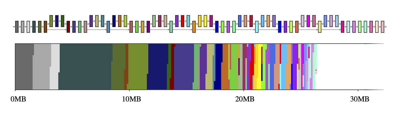 |
| Figure 1. The intermediate tensors of MobileNet v2 (top) and a mapping of their sizes onto a 2D memory space (bottom). If each intermediate tensor uses a dedicated memory buffer (depicted with 65 distinct colors), they take up ~26MB of runtime memory. |
The good news is that these intermediate tensors don’t have to co-exist in memory thanks to data dependency analysis. This allows us to reuse the memory buffers of the intermediate tensors and reduce the total memory footprint of the inference engine. If the network has the shape of a simple chain, two large memory buffers are sufficient as they can be swapped back and forth interchangeably throughout the network. However, for arbitrary networks forming complicated graphs, this NP-complete resource allocation problem requires a good approximation algorithm.
We have devised a number of different approximation algorithms for this problem, and they all perform differently depending on the neural network and the properties of memory buffers, but they all use one thing in common: tensor usage records. A tensor usage record of an intermediate tensor is an auxiliary data structure that contains information about how big the tensor is and when it is used for the first and the last time in a given execution plan of the network. With the help of these records, the memory manager is able to compute the intermediate tensor usages at any moment in the network’s execution and optimize its runtime memory for the smallest footprint possible.
Shared Memory Buffer Objects
In TFLite GPU OpenGL backend, we employ GL textures for these intermediate tensors. These come with a couple of interesting restrictions: (a) A texture’s size can’t be modified after its creation, and (b) only one shader program gets exclusive access to the texture object at a given time. In this Shared Memory Buffer Objects mode, the objective is to minimize the sum of the sizes of all created shared memory buffer objects in the object pool. This optimization is similar to the well-known register allocation problem, except that it’s much more complicated due to the variable size of each object.
With the aforementioned tensor usage records, we have devised 5 different algorithms as shown in Table 1. Except for Min-Cost Flow, they are greedy algorithms, each using a different heuristic, but still reaching or getting very close to the theoretical lower bound. Some algorithms perform better than others depending on the network topology, but in general, GREEDY_BY_SIZE_IMPROVED and GREEDY_BY_BREADTH produce the object assignments with the smallest memory footprint.
 |
| Table 1. Memory footprint of Shared Objects strategies (in MB; best results highlighted in green). The first 5 rows are our strategies, and the last 2 serve as a baseline (Lower Bound denotes an approximation of the best number possible which may not be achievable, and Naive denotes the worst number possible with each intermediate tensor assigned its own memory buffer). |
Coming back to our opening example, GREEDY_BY_BREADTH performs best on MobileNet v2 which leverages each operator’s breadth, i.e. the sum of all tensors in the operator’s profile. Figure 2, especially when compared to Figure 1, highlights how big of a gain one can get when employing a smart memory manager.
 |
| Figure 2. The intermediate tensors of MobileNet v2 (top) and a mapping of their sizes onto a 2D memory space (bottom). If the intermediate tensors share memory buffers (depicted with 4 distinct colors), they only take up ~7MB of runtime memory. |
Memory Offset Calculation
For TFLite running on the CPU, the memory buffer properties applicable to GL textures don’t apply. Thus, it is more common to allocate a huge memory arena upfront and have it shared among all readers and writers which access it by a given offset that does not interfere with other read and writes. The objective in this Memory Offset Calculation approach is to minimize the size of the memory arena.
We have devised 3 different algorithms for this optimization problem and have also explored prior work (Strip Packing by Sekiyama et al. 2018). Similar to the Shared Objects approach, some algorithms perform better than others depending on the network as shown in Table 2. One takeaway from this investigation is that the Offset Calculation approach has a smaller footprint than the Shared Objects approach in general, and thus, one should prefer the former over the latter if applicable.
 |
| Table 2. Memory footprint of Offset Calculation strategies (in MB; best results highlighted in green). The first 3 rows are our strategies, the next 1 is prior work, and the last 2 serve as baseline (Lower Bound denotes an approximation of the best number possible which may not be achievable, and Naive denotes the worst number possible with each intermediate tensor assigned its own memory buffer). |
These memory optimizations, for both CPU and GPU, have shipped by default with the last few stable TFLite releases, and have proven valuable in supporting more demanding, state-of-the-art models like MobileBERT. You can find more details about the implementation by looking at the GPU implementation and CPU implementation directly.
Acknowledgements
Matthias Grundmann, Jared Duke, Sarah Sirajuddin, and special thanks to Andrei Kulik for initial brainstorming and Terry Heo for the final implementation in TFLite.
Emine Yilmaz: An Amazon Scholar advancing the state of the art in voice shopping
Scientist leads team in London focused on improving voice-shopping experiences with Alexa.Read More

Developing Real-Time, Automatic Sign Language Detection for Video Conferencing
Posted by Amit Moryossef, Research Intern, Google Research
Video conferencing should be accessible to everyone, including users who communicate using sign language. However, since most video conference applications transition window focus to those who speak aloud, it makes it difficult for signers to “get the floor” so they can communicate easily and effectively. Enabling real-time sign language detection in video conferencing is challenging, since applications need to perform classification using the high-volume video feed as the input, which makes the task computationally heavy. In part, due to these challenges, there is only limited research on sign language detection.
In “Real-Time Sign Language Detection using Human Pose Estimation”, presented at SLRTP2020 and demoed at ECCV2020, we present a real-time sign language detection model and demonstrate how it can be used to provide video conferencing systems a mechanism to identify the person signing as the active speaker.
 |
| Maayan Gazuli, an Israeli Sign Language interpreter, demonstrates the sign language detection system. |
Our Model
To enable a real-time working solution for a variety of video conferencing applications, we needed to design a light weight model that would be simple to “plug and play.” Previous attempts to integrate models for video conferencing applications on the client side demonstrated the importance of a light-weight model that consumes fewer CPU cycles in order to minimize the effect on call quality. To reduce the input dimensionality, we isolated the information the model needs from the video in order to perform the classification of every frame.
Because sign language involves the user’s body and hands, we start by running a pose estimation model, PoseNet. This reduces the input considerably from an entire HD image to a small set of landmarks on the user’s body, including the eyes, nose, shoulders, hands, etc. We use these landmarks to calculate the frame-to-frame optical flow, which quantifies user motion for use by the model without retaining user-specific information. Each pose is normalized by the width of the person’s shoulders in order to ensure that the model attends to the person signing over a range of distances from the camera. The optical flow is then normalized by the video’s frame rate before being passed to the model.
To test this approach, we used the German Sign Language corpus (DGS), which contains long videos of people signing, and includes span annotations that indicate in which frames signing is taking place. As a naïve baseline, we trained a linear regression model to predict when a person is signing using optical flow data. This baseline reached around 80% accuracy, using only ~3μs (0.000003 seconds) of processing time per frame. By including the 50 previous frames’ optical flow as context to the linear model, it is able to reach 83.4%.
To generalize the use of context, we used a long-short-term memory (LSTM) architecture, which contains memory over the previous timesteps, but no lookback. Using a single layer LSTM, followed by a linear layer, the model achieves up to 91.5% accuracy, with 3.5ms (0.0035 seconds) of processing time per frame.
 |
| Classification model architecture. (1) Extract poses from each frame; (2) calculate the optical flow from every two consecutive frames; (3) feed through an LSTM; and (4) classify class. |
Proof of Concept
Once we had a functioning sign language detection model, we needed to devise a way to use it for triggering the active speaker function in video conferencing applications. We developed a lightweight, real-time, sign language detection web demo that connects to various video conferencing applications and can set the user as the “speaker” when they sign. This demo leverages PoseNet fast human pose estimation and sign language detection models running in the browser using tf.js, which enables it to work reliably in real-time.
When the sign language detection model determines that a user is signing, it passes an ultrasonic audio tone through a virtual audio cable, which can be detected by any video conferencing application as if the signing user is “speaking.” The audio is transmitted at 20kHz, which is normally outside the hearing range for humans. Because video conferencing applications usually detect the audio “volume” as talking rather than only detecting speech, this fools the application into thinking the user is speaking.
 |
| The sign language detection demo takes the webcam’s video feed as input, and transmits audio through a virtual microphone when it detects that the user is signing. |
You can try our experimental demo right now! By default, the demo acts as a sign language detector. The training code and models as well as the web demo source code is available on GitHub.
Demo
In the following video, we demonstrate how the model might be used. Notice the yellow chart at the top left corner, which reflects the model’s confidence in detecting that activity is indeed sign language. When the user signs, the chart values rise to nearly 100, and when she stops signing, it falls to zero. This process happens in real-time, at 30 frames per second, the maximum frame rate of the camera used.
| Maayan Gazuli, an Israeli Sign Language interpreter, demonstrates the sign language detection demo. |
User Feedback
To better understand how well the demo works in practice, we conducted a user experience study in which participants were asked to use our experimental demo during a video conference and to communicate via sign language as usual. They were also asked to sign over each other, and over speaking participants to test the speaker switching behavior. Participants responded positively that sign language was being detected and treated as audible speech, and that the demo successfully identified the signing attendee and triggered the conferencing system’s audio meter icon to draw focus to the signing attendee.
Conclusions
We believe video conferencing applications should be accessible to everyone and hope this work is a meaningful step in this direction. We have demonstrated how our model could be leveraged to empower signers to use video conferencing more conveniently.
Acknowledgements
Amit Moryossef, Ioannis Tsochantaridis, Roee Aharoni, Sarah Ebling, Annette Rios, Srini Narayanan, George Sung, Jonathan Baccash, Aidan Bryant, Pavithra Ramasamy and Maayan Gazuli

Boosting quantum computer hardware performance with TensorFlow
A guest article by Michael J. Biercuk, Harry Slatyer, and Michael Hush of Q-CTRL
Google recently announced the release of TensorFlow Quantum – a toolset for combining state-of-the-art machine learning techniques with quantum algorithm design. This was an important step to build tools for developers working on quantum applications – users operating primarily at the “top of the stack”.
In parallel we’ve been building a complementary TensorFlow-based toolset working from the hardware level up – from the bottom of the stack. Our efforts have focused on improving the performance of quantum computing hardware through the integration of a set of techniques we call quantum firmware.
In this article we’ll provide an overview of the fundamental driver for this work – combating noise and error in quantum computers – and describe how the team at Q-CTRL uses TensorFlow to efficiently characterize and suppress the impact of noise and imperfections in quantum hardware. These are key challenges in the global effort to make quantum computers useful.

The Achilles heel of quantum computers – noise and error
Quantum computing, simply put, is a new way to process information using the laws of quantum physics – the rules that govern nature on tiny size scales. Through decades of effort in science and engineering we’re now ready to put this physics to work solving problems that are exceptionally difficult for regular computers.
Realizing useful computations on today’s systems requires a recognition that performance is predominantly limited by hardware imperfections and failures, not system size. Susceptibility to noise and error remains the Achilles heel of quantum computers, and ultimately limits the range and utility of algorithms run on quantum computing hardware.
As a broad community average, most quantum computer hardware can run just a few dozen calculations over a time much less than one millisecond before requiring a reset due to the influence of noise. Depending on the specifics that’s about 1024 times worse than the hardware in a laptop!
This is the heart of why quantum computing is really hard. In this context, “noise” describes all of the things that cause interference in a quantum computer. Just like a mobile phone call can suffer interference leading it to break up, a quantum computer is susceptible to interference from all sorts of sources, like electromagnetic signals coming from WiFi or disturbances in the Earth’s magnetic field.
When qubits in a quantum computer are exposed to this kind of noise, the information in them gets degraded just the way sound quality is degraded by interference on a call. In a quantum system this process is known as decoherence. Decoherence causes the information encoded in a quantum computer to become randomized – and this leads to errors when we execute an algorithm. The greater the influence of noise, the shorter the algorithm that can be run.
So what do we do about this? To start, for the past two decades teams have been working to make their hardware more passively stable – shielding it from the noise that causes decoherence. At the same time theorists have designed a clever algorithm called Quantum Error Correction that can identify and fix errors in the hardware, based in large part on classical error correction codes. This is essential in principle, but the downside is that to make it work you have to spread the information in one qubit over lots of qubits; it may take 1000 or more physical qubits to realize just one error-corrected “logical qubit”. Today’s machines are nowhere near capable of getting benefits from this kind of Quantum Error Correction.
Q-CTRL adds something extra – quantum firmware – which can stabilize the qubits against noise and decoherence without the need for extra resources. It does this by adding new solutions at the lowest layer of the quantum computing stack that improve the hardware’s robustness to error.
Building quantum firmware with TensorFlow

Quantum firmware describes a set of protocols whose purpose is to deliver quantum hardware with augmented performance to higher levels of abstraction in the quantum computing stack. The choice of the term firmware reflects the fact that the relevant routines are usually software-defined but embedded proximal to the physical layer and effectively invisible to higher layers of abstraction.
Quantum computing hardware generally relies on a form of precisely engineered light-matter interaction in order to enact quantum logic operations. These operations in a sense constitute the native machine language for a quantum computer; a timed pulse of microwaves on resonance with a superconducting qubit can translate to an effective bit-flip operation while another pulse may implement a conditional logic operation between a pair of qubits. An appropriate composition of these electromagnetic signals then implements the target quantum algorithm.
Quantum firmware determines how the physical hardware should be manipulated, redefining the hardware machine language in a way that improves stability against decoherence. Key to this process is the calculation of noise-robust operations using information gleaned from the hardware itself.
Building in TensorFlow was essential to moving beyond “home-built’’ code to commercial-grade products for Q-CTRL. Underpinning these techniques (formally coming from the field of quantum control) are tools allowing us to perform complex gradient-based optimizations. We express all optimization problems as data flow graphs, which describe how optimization variables (variables that can be tuned by the optimizer) are transformed into the cost function (the objective that the optimizer attempts to minimize). We combine custom convenience functions with access to TensorFlow primitives in order to efficiently perform optimizations as used in many different parts of our workflow. And critically, we exploit TensorFlow’s efficient gradient calculation tools to address what is often the weakest link in home-built implementations, especially as the analytic form of the relevant function is often nonlinear and contains many complex dependencies.
For example, consider the case of defining a numerically optimized error-robust quantum bit flip used to manipulate a qubit – the analog of a classical NOT gate. As mentioned above, in a superconducting qubit this is achieved using a pulse of microwaves. We have the freedom to “shape” various aspects of the envelope of the pulse in order to enact the same mathematical transformation in a way that exhibits robustness against common noise sources, such as fluctuations in the strength or frequency of the microwaves.
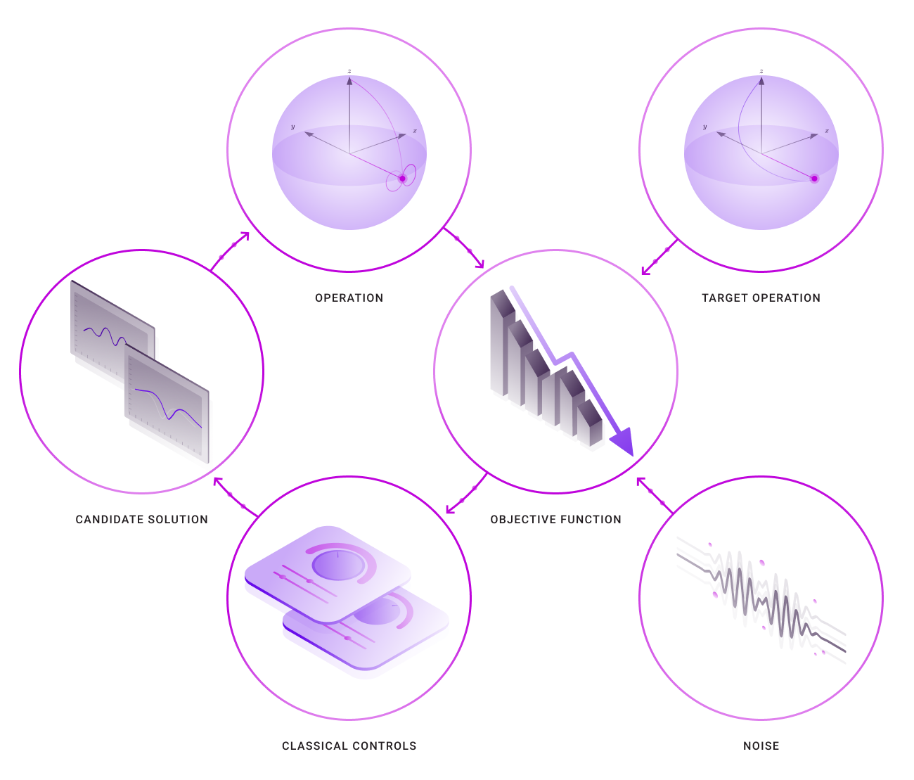
To do this we first define the data flow graph used to optimize the manipulation of this qubit – it includes objects that describe available “knobs” to adjust, the sources of noise, and the target operation (here a Hadamard gate).
|
| The data flow graph used to optimize quantum controls. The loop at left is run through our TensorFlow optimization engine |
Once the graph has been defined inside our context manager, an object must be created that ties together the objective function (in this case minimizing the resultant gate error) and the desired outputs defining the shape of the microwave pulse. With the graph object created, an optimization can be run using a service that returns a new graph object containing the results of the optimization.
This structure allows us to simply create helper functions which enable physically motivated constraints to be built directly into the graph. For instance, these might be symmetry requirements, limits on how a signal changes in time, or even incorporation of characteristics of the electronics systems used to generate the microwave pulses. Any other capabilities not directly covered by this library of helper functions can also be directly coded as TensorFlow primitives.
With this approach we achieve an extremely flexible and high-performance optimization engine; our direct benchmarking has revealed order-of-magnitude benefits in time to solution relative to the best available alternative architectures.
The capabilities enabled by this toolkit span the space of tasks required to stabilize quantum computing hardware and reduce errors at the lowest layer of the quantum computing stack. And importantly they’re experimentally verified on real quantum computing hardware; quantum firmware has been shown to reduce the likelihood of errors, mitigate system performance variations across devices, stabilize hardware against slowly drifting out of calibration, and even make quantum logic operations more compatible with higher level abstractions in quantum computing such as quantum error correction. All of these capabilities and real hardware demonstrations are accessible via our publicly available User Guides and Application Notes in executable Jupyter notebook form.
Ultimately, we believe that building and operating large-scale quantum computing systems will be effectively impossible without the integration of the capabilities encapsulated in quantum firmware. There are many concepts to be drawn from across the fields of machine learning and robotic control in the drive for performance and autonomy, and TensorFlow has proven an efficient language to support the development of the critical toolsets.
A brief history of QC, from Shor to quantum machine learning
The quantum computing boom started in 1994 with the discovery of Shor’s algorithm for factoring large numbers. Public key cryptosystems — which is to say, most encryption — rely on the mathematical complexity of factoring primes to keep messages safe from prying computers. By virtue of their approach to encoding and processing information, however, quantum computers are conjectured to be able to factor primes faster — exponentially faster — than a classical machine. In principle this poses an existential threat not only to national security, but also emerging technologies such as cryptocurrencies.
This realization set in motion the development of the entire field of quantum computing. Shor’s algorithm spurred the NSA to begin one of its first ever open, University-driven research programs asking the question of whether such systems could be built. Fast forward to 2020 and quantum supremacy has been achieved, meaning that a real quantum computing hardware system has performed a task that’s effectively impossible for even the world’s largest supercomputers.
Quantum supremacy is an important technical milestone whose practical importance in solving problems of relevance to end users remains a bit unclear. Our community is continuing to make great progress towards quantum advantage – a threshold indicating that it’s actually cheaper or faster to use a quantum computer for a problem of practical relevance. And for the right problems, we think that within the next 5-10 years we’ll cross that threshold with a quantum computer that isn’t that much bigger than the ones we have today. It just needs to perform much better.
So, which problems are the right problems for quantum computers to address first?
In many respects, Shor’s algorithm has receded in importance as the scale of the challenge emerged. A recent technical analysis suggests that we’re unlikely to see Shor deployed at a useful scale until 2039. Today, small-scale machines with a couple of dozen interacting qubits exist in labs around the world, built from superconducting circuits, individual trapped atoms, or similarly exotic materials. The problem is that these early machines are just too small and too fragile to solve problems relevant to factoring.
To factor a number sufficiently large to be relevant in cryptography, one would need a system composed of thousands of qubits capable of handling trillions of operations each. This is nothing for a conventional machine where hardware can run for a billion years at a billion operations per second and never be likely to suffer a fault. But as we’ve seen it’s quite a different story for quantum computers.
These limits have driven the emergence of a new class of applications in materials science and chemistry that could prove equally impactful, using much smaller systems. Quantum computing in the near term could also help develop new classes of artificial intelligence systems. Recent efforts have demonstrated a strong and unexpected link between quantum computation and artificial neural networks, potentially portending new approaches to machine learning.
This class of problem can often be cast as optimizations where input into a classical machine learning algorithm comes from a small quantum computation, or where data is represented in the quantum domain and a learning procedure implemented. TensorFlow Quantum provides an exciting toolset for developers seeking new and improved ways to exploit the small quantum computers existing now and in the near future.
Still, even those small machines don’t perform particularly well. Q-CTRL’s quantum firmware enables users to extract maximum performance from hardware. Thus we see that TensorFlow has a critical role to play across the emerging quantum computing software stack – from quantum firmware through to algorithms for quantum machine learning.
Resources if you’d like to learn more
We appreciate that members of the TensorFlow community may have varying levels of familiarity with quantum computing, and that this overview was only a starting point. To help readers interested in learning more about quantum computing we’re happy to provide a few resources:
- For those knowledgeable about machine learning, Q-CTRL has also produced a series of webinars introducing the concept of Robust Control in quantum computing and even demonstrating reinforcement learning to discover gates on real quantum hardware.
- If you need to start from zero, Q-CTRL has produced a series of introductory video tutorials helping the uninitiated begin their quantum journey via our learning center. We also offer a visual interface enabling new users to discover and build intuition for the core concepts underlying quantum computing – including the impact of noise on quantum hardware.
- Jack Hidary from X wrote a great text focused on linking the foundations of quantum computing with how teams today write code for quantum machines.
- The traditional “formal” starting point for those interested in quantum computing is the timeless textbook from “Mike and Ike”

Audiovisual Speech Enhancement in YouTube Stories
Posted by Inbar Mosseri, Software Engineer and Michael Rubinstein, Research Scientist, Google Research
While tremendous efforts are invested in improving the quality of videos taken with smartphone cameras, the quality of audio in videos is often overlooked. For example, the speech of a subject in a video where there are multiple people speaking or where there is high background noise might be muddled, distorted, or difficult to understand. In an effort to address this, two years ago we introduced Looking to Listen, a machine learning (ML) technology that uses both visual and audio cues to isolate the speech of a video’s subject. By training the model on a large-scale collection of online videos, we are able to capture correlations between speech and visual signals such as mouth movements and facial expressions, which can then be used to separate the speech of one person in a video from another, or to separate speech from background sounds. We showed that this technology not only achieves state-of-the-art results in speech separation and enhancement (a noticeable 1.5dB improvement over audio-only models), but in particular can improve the results over audio-only processing when there are multiple people speaking, as the visual cues in the video help determine who is saying what.
We are now happy to make the Looking to Listen technology available to users through a new audiovisual Speech Enhancement feature in YouTube Stories (on iOS), allowing creators to take better selfie videos by automatically enhancing their voices and reducing background noise. Getting this technology into users’ hands was no easy feat. Over the past year, we worked closely with users to learn how they would like to use such a feature, in what scenarios, and what balance of speech and background sounds they would like to have in their videos. We heavily optimized the Looking to Listen model to make it run efficiently on mobile devices, overall reducing the running time from 10x real-time on a desktop when our paper came out, to 0.5x real-time performance on the phone. We also put the technology through extensive testing to verify that it performs consistently across different recording conditions and for people with different appearances and voices.
From Research to Product
Optimizing Looking to Listen to allow fast and robust operation on mobile devices required us to overcome a number of challenges. First, all processing needed to be done on-device within the client app in order to minimize processing time and to preserve the user’s privacy; no audio or video information would be sent to servers for processing. Further, the model needed to co-exist alongside other ML algorithms used in the YouTube app in addition to the resource-consuming video recording itself. Finally, the algorithm needed to run quickly and efficiently on-device while minimizing battery consumption.
The first step in the Looking to Listen pipeline is to isolate thumbnail images that contain the faces of the speakers from the video stream. By leveraging MediaPipe BlazeFace with GPU accelerated inference, this step is now able to be executed in just a few milliseconds. We then switched the model part that processes each thumbnail separately to a lighter weight MobileNet (v2) architecture, which outputs visual features learned for the purpose of speech enhancement, extracted from the face thumbnails in 10 ms per frame. Because the compute time to embed the visual features is short, it can be done while the video is still being recorded. This avoids the need to keep the frames in memory for further processing, thereby reducing the overall memory footprint. Then, after the video finishes recording, the audio and the computed visual features are streamed to the audio-visual speech separation model which produces the isolated and enhanced speech.
We reduced the total number of parameters in the audio-visual model by replacing “regular” 2D convolutions with separable ones (1D in the frequency dimension, followed by 1D in the time dimension) with fewer filters. We then optimized the model further using TensorFlow Lite — a set of tools that enable running TensorFlow models on mobile devices with low latency and a small binary size. Finally, we reimplemented the model within the Learn2Compress framework in order to take advantage of built-in quantized training and QRNN support.
 |
| Our Looking to Listen on-device pipeline for audiovisual speech enhancement |
These optimizations and improvements reduced the running time from 10x real-time on a desktop using the original formulation of Looking to Listen, to 0.5x real-time performance using only an iPhone CPU; and brought the model size down from 120MB to 6MB now, which makes it easier to deploy. Since YouTube Stories videos are short — limited to 15 seconds — the result of the video processing is available within a couple of seconds after the recording is finished.
Finally, to avoid processing videos with clean speech (so as to avoid unnecessary computation), we first run our model only on the first two seconds of the video, then compare the speech-enhanced output to the original input audio. If there is sufficient difference (meaning the model cleaned up the speech), then we enhance the speech throughout the rest of the video.
Researching User Needs
Early versions of Looking to Listen were designed to entirely isolate speech from the background noise. In a user study conducted together with YouTube, we found that users prefer to leave in some of the background sounds to give context and to retain some the general ambiance of the scene. Based on this user study, we take a linear combination of the original audio and our produced clean speech channel: output_audio = 0.1 x original_audio + 0.9 x speech. The following video presents clean speech combined with different levels of the background sounds in the scene (10% background is the balance we use in practice).
Below are additional examples of the enhanced speech results from the new Speech Enhancement feature in YouTube Stories. We recommend watching the videos with good speakers or headphones.
Fairness Analysis
Another important requirement is that the model be fair and inclusive. It must be able to handle different types of voices, languages and accents, as well as different visual appearances. To this end, we conducted a series of tests exploring the performance of the model with respect to various visual and speech/auditory attributes: the speaker’s age, skin tone, spoken language, voice pitch, visibility of the speaker’s face (% of video in which the speaker is in frame), head pose throughout the video, facial hair, presence of glasses, and the level of background noise in the (input) video.
For each of the above visual/auditory attributes, we ran our model on segments from our evaluation set (separate from the training set) and measured the speech enhancement accuracy, broken down according to the different attribute values. Results for some of the attributes are summarized in the following plots. Each data point in the plots represents hundreds (in most cases thousands) of videos fitting the criteria.
 |
| Speech enhancement quality (signal-to-distortion ratio, SDR, in dB) for different spoken languages, sorted alphabetically. The average SDR was 7.89 dB with a standard deviation of 0.42 dB — deviation that for human listeners is considered hard to notice. |
 |
| Left: Speech enhancement quality as a function of the speaker’s voice pitch. The fundamental voice frequency (pitch) of an adult male typically ranges from 85 to 180 Hz, and that of an adult female ranges from 165 to 255 Hz. Right: speech enhancement quality as a function of the speaker’s predicted age. |
 |
| As our method utilizes facial cues and mouth movements to isolate the speech, we tested whether facial hair (e.g., a moustache, beard) may obstruct those visual cues and affect the method’s performance. Our evaluations show that the quality of speech enhancement is maintained well also in the presence of facial hair. |
Using the Feature
YouTube creators who are eligible for YouTube Stories creation may record a video on iOS, and select “Enhance speech” from the volume controls editing tool. This will immediately apply speech enhancement to the audio track and will play back the enhanced speech in a loop. It is then possible to toggle the feature on and off multiple times to compare the enhanced speech with the original audio.

In parallel to this new feature in YouTube, we are also exploring additional venues for this technology. More to come later this year — stay tuned!
Acknowledgements
This feature is a collaboration across multiple teams at Google. Key contributors include: from Research-IL: Oran Lang; from VisCAM: Ariel Ephrat, Mike Krainin, JD Velasquez, Inbar Mosseri, Michael Rubinstein; from Learn2Compress: Arun Kandoor; from MediaPipe: Buck Bourdon, Matsvei Zhdanovich, Matthias Grundmann; from YouTube: Andy Poes, Vadim Lavrusik, Aaron La Lau, Willi Geiger, Simona De Rosa, and Tomer Margolin.

What if you could turn your voice into any instrument?
Imagine whistling your favorite song. You might not sound like the real deal, right? Now imagine your rendition using auto-tune software. Better, sure, but the result is still your voice. What if there was a way to turn your voice into something like a violin, or a saxophone, or a flute?
Google Research’s Magenta team, which has been focused on the intersection of machine learning and creative tools for musicians, has been experimenting with exactly this. The team recently created an open source technology called Differentiable Digital Signal Processing (DDSP). DDSP is a new approach to machine learning that enables models to learn the characteristics of a musical instrument and map them to a different sound. The process can lead to so many creative, quirky results. Try replacing a capella singing with a saxophone solo, or a dog barking with a trumpet performance. The options are endless.
And so are the sounds you can make. This development is important because it enables music technologies to become more inclusive. Machine learning models inherit biases from the datasets they are trained on, and music models are no different. Many are trained on the structure of western musical scores, which excludes much of the music from the rest of the world. Rather than following the formal rules of western music, like the 12 notes on a piano, DDSP transforms sound by modeling frequencies in the audio itself. This opens up machine learning technologies to a wider range of musical cultures.
In fact, anyone can give it a try. We created a tool called Tone Transfer to allow musicians and amateurs alike to tap into DDSP as a delightful creative tool. Play with the Tone Transfer showcase to sample sounds, or record your own, and listen to how they can be transformed into a myriad of instruments using DDSP technology. Check out our film that shows artists using Tone Transfer for the first time.
DDSP does not create music on its own; think of it like another instrument that requires skill and thought. It’s an experimental soundscape environment for music, and we’re so excited to see how the world uses it.
Say goodbye to hold music
Sometimes, a phone call is the best way to get something done. We call retailers to locate missing packages, utilities to adjust our internet speeds, airlines to change our travel itineraries…the list goes on. But more often than not, we need to wait on hold during these calls—listening closely to hold music and repetitive messages—before we reach a customer support representative who can help. In fact, people in the United States spent over 10 million hours on hold with businesses last week.
Save time with Hold for Me
Hold for Me, our latest Phone app feature, helps you get that time back, starting with an early preview on Pixel 5 and Pixel 4a (5G) in the U.S. Now, when you call a toll-free number and a business puts you on hold, Google Assistant can wait on the line for you. You can go back to your day, and Google Assistant will notify you with sound, vibration and a prompt on your screen once someone is on the line and ready to talk. That means you’ll spend more time doing what’s important to you, and less time listening to hold music.

Tap “Hold for me” in Google’s Phone app after you’re placed on hold by a business.
Hold for Me is our latest effort to make phone calls better and save you time. Last year, we introduced an update to Call Screen that helps you avoid interruptions from spam calls once and for all, and last month, we launched Verified Calls to help you know why a business is calling before you answer. Hold for Me is now another way we’re making it simpler to say hello.
Powered by Google AI
Every business’s hold loop is different and simple algorithms can’t accurately detect when a customer support representative comes onto the call. Hold for Me is powered by Google’s Duplex technology, which not only recognizes hold music but also understands the difference between a recorded message (like “Hello, thank you for waiting”) and a representative on the line. Once a representative is identified, Google Assistant will notify you that someone’s ready to talk and ask the representative to hold for a moment while you return to the call. We gathered feedback from a number of companies, including Dell and United, as well as from studies with customer support representatives, to help us design these interactions and make the feature as helpful as possible to the people on both sides of the call.
While Google Assistant waits on hold for you, Google’s natural language understanding also keeps you informed. Your call will be muted to let you focus on something else, but at any time, you can check real-time captions on your screen to know what’s happening on the call.
Keeping your data safe
Hold for Me is an optional feature you can enable in settings and choose to activate during each call to a toll-free number. To determine when a representative is on the line, audio is processed entirely on your device and does not require a Wi-Fi or data connection. This makes the experience fast and also protects your privacy—no audio from the call will be shared with Google or saved to your Google account unless you explicitly decide to share it and help improve the feature. When you return to the call after Google Assistant was on hold for you, audio stops being processed altogether.
We’re excited to bring an early preview of Hold for Me to our latest Pixel devices and continue making the experience better over time. Your feedback will help us bring the feature to more people over the coming months, so they too can say goodbye to hold music and say hello to more free time.

How The Trevor Project continues to support LGBTQ youth
This September, National Suicide Prevention Awareness Month feels different. Over the past nine months, LGBTQ youth have experienced unique challenges in relation to COVID-19.The pandemic has amplified existing mental health disparities and created new problems that have impacted the daily lives of many LGBTQ youth.
As the world’s largest suicide prevention and crisis intervention organization for LGBTQ young people, The Trevor Project has seen the volume of youth reaching out to our crisis services for support increase significantly, at times double our pre-COVID volume. We’ve heard from a great number of youth who no longer have access to their usual support systems, including many who have been forced to confine in unsupportive home environments. The unprecedented crisis of 2020 has reaffirmed the need for increased mental health support for LGBTQ youth, particularly as we’ve ventured into a more virtual world.
From transitioning our physical call center operations to be fully remote to publishing aresource to help LGBTQ youth explore conversations around the intersection of their racial and LGBTQ identities—The Trevor Project has remained open and responsive to the needs of the young people we serve despite the onslaught of challenges. Technological advancement has been essential as Trevor adapts to meet this moment. In particular, artificial intelligence (AI) is a crucial component for scaling our services to support the increase of youth reaching out.
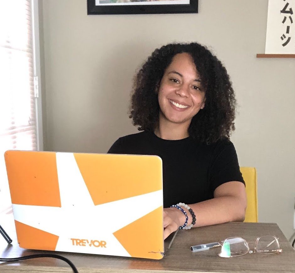
Kendra Gaunt joined The Trevor Project nine months ago as a Data and AI product owner.
I joined The Trevor Project as the Data and AI product owner nine months ago, and started working alongside our AI and engineering team and 11 Google.org Fellows who were doing six months of full-time pro bono work with us. With the support of $2.7 million in Google.org grant funding and two teams of pro bono Google.org Fellows, we have introduced new AI applications to scale our impact. We built an AI system that helps us identify which LGBTQ individuals reaching out to us for support are at the highest risk of suicide so that we can quickly connect them to counselors who are ready to help at that moment. And now, we’re leveraging AI to ensure the safety of our TrevorSpace forums through auto-moderation, and to train more volunteer counselors through a conversation simulator. It’s projects like these that have enabled The Trevor Project to directly serve more than 150,000 crisis contacts from LGBTQ youth in the past year.
And we’re just getting started. With the guidance of best practices from Google, we’re significantly growing our in-house AI team. As we grow and develop a long-term product strategy around our use of data and AI, we acknowledge our responsibility to create a values-based system to guide how we use and develop AI. By applying learnings from Google’s Responsible Innovation team, we created a set of principles to ensure that we develop models that avoid reinforcing unfair bias that impacts people based on their ethnicity, sexual orientation, gender identity, race, and the intersection of these identities.
I joined The Trevor Project because it’s an organization driven by values, and our use of technology reflects this. I noticed an opportunity to leverage my years of experience and partner with people who are committed to employing technology for social good. Through the thoughtful and ethical use of AI, we can overcome obstacles of scale and complexity as we pursue our mission to end suicide among LGBTQ youth.
To learn more about National Suicide Prevention Awareness Month and the work The Trevor Project is doing, check out ourCARE campaign. This includes actionable steps anyone can take to support their community and prevent suicide, as well as technological innovations that help us serve more young people, faster.
If you or someone you know needs help or support, contact The Trevor Project’s TrevorLifeline 24/7 at 1-866-488-7386. Counseling is also available 24/7 via chat every day at TheTrevorProject.org/help or by texting 678-678.