PyTorch is a machine learning (ML) framework that is widely used by AWS customers for a variety of applications, such as computer vision, natural language processing, content creation, and more. With the recent PyTorch 2.0 release, AWS customers can now do same things as they could with PyTorch 1.x but faster and at scale with improved training speeds, lower memory usage, and enhanced distributed capabilities. Several new technologies including torch.compile, TorchDynamo, AOTAutograd, PrimTorch, and TorchInductor have been included in the PyTorch2.0 release. Refer to PyTorch 2.0: Our next generation release that is faster, more Pythonic and Dynamic as ever for details.
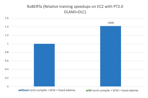
This post demonstrates the performance and ease of running large-scale, high-performance distributed ML model training and deployment using PyTorch 2.0 on AWS. This post further walks through a step-by-step implementation of fine-tuning a RoBERTa (Robustly Optimized BERT Pretraining Approach) model for sentiment analysis using AWS Deep Learning AMIs (AWS DLAMI) and AWS Deep Learning Containers (DLCs) on Amazon Elastic Compute Cloud (Amazon EC2 p4d.24xlarge) with an observed 42% speedup when used with PyTorch 2.0 torch.compile + bf16 + fused AdamW. The fine-tuned model is then deployed on AWS Graviton-based C7g EC2 instance on Amazon SageMaker with an observed 10% speedup compared to PyTorch 1.13.
The following figure shows a performance benchmark of fine-tuning a RoBERTa model on Amazon EC2 p4d.24xlarge with AWS PyTorch 2.0 DLAMI + DLC.
Refer to Optimized PyTorch 2.0 inference with AWS Graviton processors for details on AWS Graviton-based instance inference performance benchmarks for PyTorch 2.0.
Support for PyTorch 2.0 on AWS
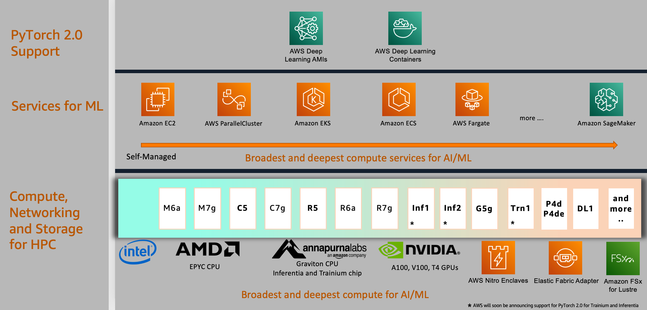
PyTorch2.0 support is not limited to the services and compute shown in example use-case in this post; it extends to many others on AWS, which we discuss in this section.
Business requirement
Many AWS customers, across a diverse set of industries, are transforming their businesses by using artificial intelligence (AI), specifically in the area of generative AI and large language models (LLMs) that are designed to generate human-like text. These are basically big models based on deep learning techniques that are trained with hundreds of billions of parameters. The growth in model sizes is increasing training time from days to weeks, and even months in some cases. This is driving an exponential increase in training and inference costs, which requires, more than ever, a framework such as PyTorch 2.0 with built-in support of accelerated model training and the optimized infrastructure of AWS tailored to the specific workloads and performance needs.
Choice of compute
AWS provides PyTorch 2.0 support on the broadest choice of powerful compute, high-speed networking, and scalable high-performance storage options that you can use for any ML project or application and customize to fit your performance and budget requirements. This is manifested in the diagram in the next section; in the bottom tier, we provide a broad selection of compute instances powered by AWS Graviton, Nvidia, AMD, and Intel processors.
For model deployments, you can use ARM-based processors such as the recently announced AWS Graviton-based instance that provides inference performance for PyTorch 2.0 with up to 3.5 times the speed for Resnet50 compared to the previous PyTorch release, and up to 1.4 times the speed for BERT, making AWS Graviton-based instances the fastest compute-optimized instances on AWS for CPU-based model inference solutions.
Choice of ML services
To use AWS compute, you can select from a broad set of global cloud-based services for ML development, compute, and workflow orchestration. This choice allows you to align with your business and cloud strategies and run PyTorch 2.0 jobs on the platform of your choice. For instance, if you have on-premises restrictions or existing investments in open-source products, you can use Amazon EC2, AWS ParallelCluster, or AWS UltraCluster to run distributed training workloads based on a self-managed approach. You could also use a fully managed service like SageMaker for a cost-optimized, fully managed, and production-scale training infrastructure. SageMaker also integrates with various MLOps tools, which allows you to scale your model deployment, reduce inference costs, manage models more effectively in production, and reduce operational burden.
Similarly, if you have existing Kubernetes investments, you can also use Amazon Elastic Kubernetes Service (Amazon EKS) and Kubeflow on AWS to implement an ML pipeline for distributed training or use an AWS-native container orchestration service like Amazon Elastic Container Service (Amazon ECS) for model training and deployments. Options to build your ML platform are not limited to these services; you can pick and choose depending on your organizational requirements for your PyTorch 2.0 jobs.
Enabling PyTorch 2.0 with AWS DLAMI and AWS DLC
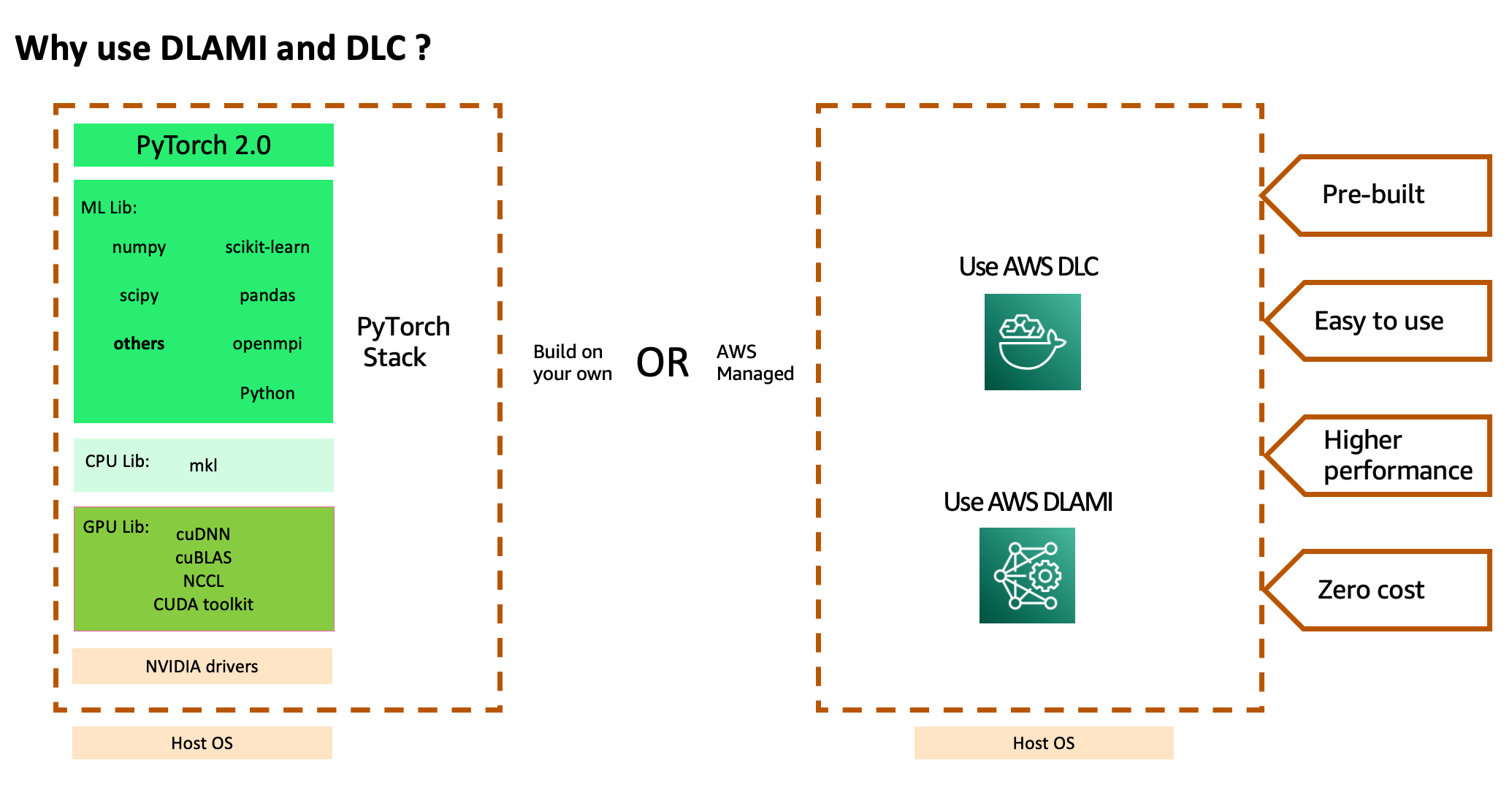
To use the aforementioned stack of AWS services and powerful compute, you have to install an optimized compiled version of the PyTorch2.0 framework and its required dependencies, many of which are independent projects, and test them end to end. You may also need CPU-specific libraries for accelerated math routines, GPU-specific libraries for accelerated math and inter-GPU communication routines, and GPU drivers that need to be aligned with the GPU compiler used to compile the GPU libraries. If your jobs require large-scale multi-node training, you need an optimized network that can provide lowest latency and highest throughput. After you build your stack, you need to regularly scan and patch them for security vulnerabilities and rebuild and retest the stack after every framework version upgrade.
AWS helps reduce this heavy lifting by offering a curated and secure set of frameworks, dependencies, and tools to accelerate deep learning in the cloud though AWS DLAMIs and AWS DLCs. These pre-built and tested machine images and containers are optimized for deep learning on EC2 Accelerated Computing Instance types, allowing you to scale out to multiple nodes for distributed workloads more efficiently and easily. It includes a pre-built Elastic Fabric Adapter (EFA), Nvidia GPU stack, and many deep learning frameworks (TensorFlow, MXNet, and PyTorch with latest release of 2.0) for high-performance distributed deep learning training. You don’t need to spend time installing and troubleshooting deep learning software and drivers or building ML infrastructure, nor do you have to incur the recurring cost of patching these images for security vulnerabilities or recreating the images after every new framework version upgrade. Instead, you can focus on the higher value-added effort of training jobs at scale in a shorter amount of time and iterating on your ML models faster.
Solution overview
Considering that training on GPU and inference on CPU is a popular use case for AWS customers, we have included as part of this post a step-by-step implementation of a hybrid architecture (as shown in the following diagram). We will explore the art-of-the-possible and use a P4 EC2 instance with BF16 support initialized with Base GPU DLAMI including NVIDIA drivers, CUDA, NCCL, EFA stack, and PyTorch2.0 DLC for fine-tuning a RoBERTa sentiment analysis model that gives you control and flexibility to use any open-source or proprietary libraries. Then we use SageMaker for a fully managed model hosting infrastructure to host our model on AWS Graviton3-based C7g instances. We picked C7g on SageMaker because it’s proven to reduce inference costs by up to 50% relative to comparable EC2 instances for real-time inference on SageMaker. The following diagram illustrates this architecture.
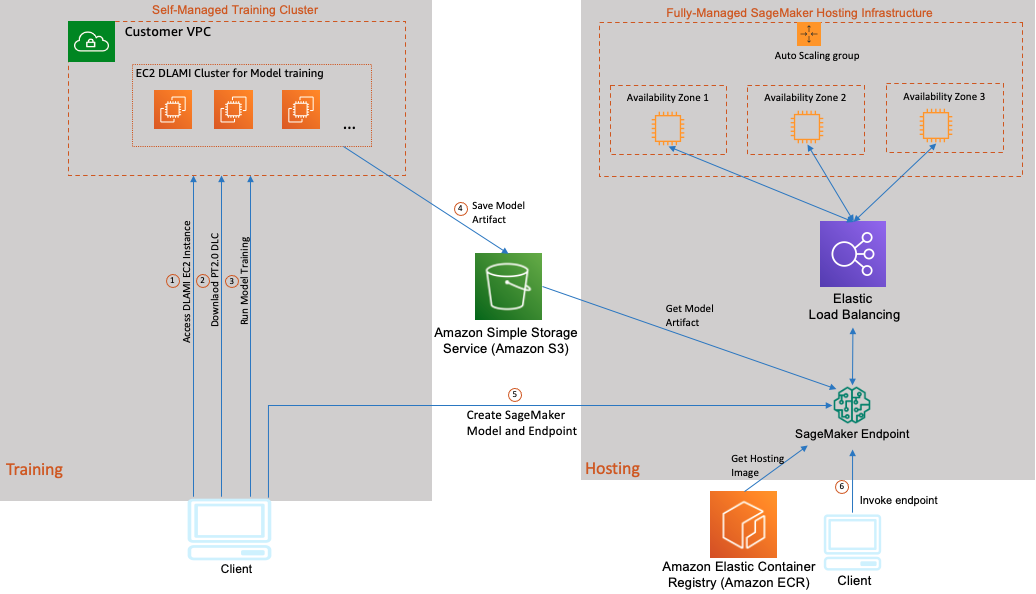
The model training and hosting in this use case consists of the following steps:
- Launch a GPU DLAMI-based EC2 Ubuntu instance in your VPC and connect to your instance using SSH.
- After you log in to your EC2 instance, download the AWS PyTorch 2.0 DLC.
- Run your DLC container with a model training script to fine-tune the RoBERTa model.
- After model training is complete, package the saved model, inference scripts, and a few metadata files into a tar file that SageMaker inference can use and upload the model package to an Amazon Simple Storage Service (Amazon S3) bucket.
- Deploy the model using SageMaker and create an HTTPS inference endpoint. The SageMaker inference endpoint holds a load balancer and one or more instances of your inference container in different Availability Zones. You can deploy either multiple versions of the same model or entirely different models behind this single endpoint. In this example, we host a single model.
- Invoke your model endpoint by sending it test data and verify the inference output.
In the following sections, we showcase fine-tuning a RoBERTa model for sentiment analysis. RoBERTa is developed by Facebook AI, improving on the popular BERT model by modifying key hyperparameters and pre-training on a larger corpus. This leads to improved performance compared to vanilla BERT.
We use the transformers library by Hugging Face to get the RoBERTa model pre-trained on approximately 124 million tweets, and we fine-tune it on the Twitter dataset for sentiment analysis.
Prerequisites
Make sure you meet the following prerequisites:
- You have an AWS account.
- Make sure you’re in the
us-west-2 Region to run this example. (This example is tested in us-west-2; however, you can run in any other Region.)
- Create a role with the name
sagemakerrole. Add managed policies AmazonSageMakerFullAccess and AmazonS3FullAccess to give SageMaker access to S3 buckets.
- Create an EC2 role with the name
ec2_role. Use the following permission policy:
#Refer - Make sure EC2 role has following policies
{
  "Version": "2012-10-17",
  "Statement": [
    {
      "Sid": "VisualEditor0",
      "Effect": "Allow",
      "Action": [
        "ecr:BatchGetImage",
        "ecr:BatchCheckLayerAvailability",
        "ecr:CompleteLayerUpload",
        "ecr:GetDownloadUrlForLayer",
        "ecr:InitiateLayerUpload",
        "ecr:PutImage",
        "ecr:UploadLayerPart",
        "ecr:GetAuthorizationToken",
        "s3:*",
        "s3-object-lambda:*",
        "iam:Get*",
        "iam:PassRole",
        "sagemaker:*"
      ],
      "Resource": "*"
    }
  ]
}
1. Launch your development instance
We create a p4d.24xlarge instance that offers 8 NVIDIA A100 Tensor Core GPUs in us-west-2:
When selecting the AMI, follow the release notes to run this command using the AWS Command Line Interface (AWS CLI) to find the AMI ID to use in us-west-2:
#STEP 1.2 - This requires AWS CLI credentials to call ec2 describe-images api (ec2:DescribeImages).
aws ec2 describe-images --region us-west-2 --owners amazon --filters 'Name=name,Values=Deep Learning Base GPU AMI (Ubuntu 20.04) ????????' 'Name=state,Values=available' --query 'reverse(sort_by(Images, &CreationDate))[:1].ImageId' --output text
Make sure the size of the gp3 root volume is 200 GiB.
EBS volume encryption is not enabled by default. Consider changing this when moving this solution to production.
2. Download a Deep Learning Container
AWS DLCs are available as Docker images in Amazon Elastic Container Registry Public, a managed AWS container image registry service that is secure, scalable, and reliable. Each Docker image is built for training or inference on a specific deep learning framework version, Python version, with CPU or GPU support. Select the PyTorch 2.0 framework from the list of available Deep Learning Containers images.
Complete the following steps to download your DLC:
a. SSH to the instance. By default, security group used with EC2 opens up SSH port to all. Please consider this if you are moving this solution to production:
#STEP 2.1 - Use Public IP
ssh -i ~/.ssh/<pub_key> ubuntu@<IP_ADDR>

#Refer - Output: Notice python3.9 package that we will use to run and install Inference scripts

__| __|_ )
_| ( / Deep Learning Base GPU AMI (Ubuntu 20.04)
___|___|___|

Welcome to Ubuntu 20.04.6 LTS (GNU/Linux 5.15.0-1035-aws x86_64v)

* Please note that Amazon EC2 P2 Instance is not supported on current DLAMI.
* Supported EC2 instances: G3, P3, P3dn, P4d, P4de, G5, G4dn.
NVIDIA driver version: 525.85.12
Default CUDA version: 11.2

Utility libraries are installed in /usr/bin/python3.9.
To access them, use /usr/bin/python3.9.
By default, the security group used with Amazon EC2 opens up the SSH port to all. Consider changing this if you are moving this solution to production.
b. Set the environment variables required to run the remaining steps of this implementation:
#STEP 2.2
Attach the role “ec2_role” to your EC2 instance from the AWS console.

#STEP 2.3
Follow the steps here to create a S3 bucket in us-west-2 region

#STEP 2.4 - Set Environment variables
#Bucket created in step 2.3
export S3_BUCKET=<your-s3-bucket>
export PYTHON_V=python3.9
export SAGEMAKER_ROLE=$(aws iam get-role --role-name sagemakerrole --output text --query 'Role.Arn')
aws configure set default.region 'us-west-2'
Amazon ECR supports public image repositories with resource-based permissions using AWS Identity and Access Management (IAM) so that specific users or services can access images.
c. Log in to the DLC registry:
#STEP 2.5 - login
aws ecr get-login-password --region us-west-2 | docker login --username AWS --password-stdin 763104351884.dkr.ecr.us-west-2.amazonaws.com

#Refer - Output
Login Succeeded
d. Pull the latest PyTorch 2.0 container with GPU support in us-west-2
#STEP 2.6 - pull the latest DLC PyTorch image
docker pull 763104351884.dkr.ecr.us-west-2.amazonaws.com/pytorch-training:2.0.0-gpu-py310-cu118-ubuntu20.04-ec2

#Refer - Output
7608715873ec: Pull complete
a0bad51e1731: Pull complete
f7778ea3b9cc: Pull complete
....

Digest: sha256:1ab0d477345a11970d811cc252bc461dd70859f15caa19a65198e7941953e6b8
StaRefertus: Downloaded newer image for 763104351884.dkr.ecr.us-west-2.amazonaws.com/pytorch-training:2.0.0-gpu-py310-cu118-ubuntu20.04-ec2
763104351884.dkr.ecr.us-west-2.amazonaws.com/pytorch-training:2.0.0-gpu-py310-cu118-ubuntu20.04-ec2
If you get the error “no space left on device”, make sure you increase the EC2 EBS volume to 200 GiB and then extend the Linux file system.
3. Clone the latest scripts adapted to PyTorch 2.0
Clone the scripts with the following code:
#STEP 3.1
cd $HOME
git clone https://github.com/aws-samples/aws-deeplearning-labs.git
cd aws-deeplearning-labs/workshop/twitter_lm/scripts/
export ml_working_dir=$PWD
Because we’re using the Hugging Face transformers API with the latest version 4.28.1, it has already enabled PyTorch 2.0 support. We added the following argument to the trainer API in train_sentiment.py to enable new PyTorch 2.0 features:
- Torch compile – Experience an average 43% speedup on Nvidia A100 GPUs with single line of change.
- BF16 datatype – New data type support (Brain Floating Point) for Ampere or newer GPUs.
- Fused AdamW optimizer – Fused AdamW implementation to further speed up training. This stochastic optimization method modifies the typical implementation of weight decay in Adam by decoupling weight decay from the gradient update.
#Refer - updated training config
training_args = TrainingArguments(
do_eval=True,
evaluation_strategy='epoch',
output_dir='test_trainer',
logging_dir='test_trainer',
logging_strategy='epoch',
save_strategy='epoch',
num_train_epochs=10,
learning_rate=1e-05,
# pytorch 2.0.0 specific args
torch_compile=True,
bf16=True,
optim='adamw_torch_fused',
per_device_train_batch_size=16,
per_device_eval_batch_size=16,
load_best_model_at_end=True,
metric_for_best_model='recall',
)
4. Build a new Docker image with dependencies
We extend the pre-built PyTorch 2.0 DLC image to install the Hugging Face transformer and other libraries that we need to fine-tune our model. This allows you to use the included tested and optimized deep learning libraries and settings without having to create an image from scratch. See the following code:
#STEP 4.1 - Create Dockerfile with following content
printf 'FROM 763104351884.dkr.ecr.us-west-2.amazonaws.com/pytorch-training:2.0.0-gpu-py310-cu118-ubuntu20.04-ec2
RUN pip install scikit-learn evaluate transformers xformers
' > Dockerfile

#STEP 4.2 - Build new docker file
docker build -f Dockerfile -t pytorch2.0:roberta-sentiment-analysis .
5. Start training using the container
Run the following Docker command to begin fine-tuning the model on the tweet_eval sentiment dataset. We’re using the Docker container arguments (shared memory size, max locked memory, and stack size) recommend by Nvidia for deep learning workloads.
#STEP 5.1 - run docker container for model training
docker run --net=host --uts=host --ipc=host --shm-size=1g --ulimit stack=67108864 --ulimit memlock=-1 --gpus all -v "/home/ubuntu:/workspace" pytorch2.0:roberta-sentiment-analysis python /workspace/aws-deeplearning-labs/workshop/twitter_lm/scripts/train_sentiment.py
You should expect the following output. The script first downloads the TweetEval dataset, which consists of seven heterogenous tasks in Twitter, all framed as multi-class tweet classification. The tasks include irony, hate, offensive, stance, emoji, emotion, and sentiment.
The script then downloads the base model and starts the fine-tuning process. Training and evaluation metrics are reported at the end of each epoch.
#Refer - Output
{'loss': 0.6927, 'learning_rate': 9e-06, 'epoch': 1.0}
{'eval_loss': 0.6144512295722961, 'eval_recall': 0.7129473901625799, 'eval_runtime': 3.2694, 'eval_samples_per_second': 611.74, 'eval_steps_per_second': 4.894, 'epoch': 1.0}
{'loss': 0.5554, 'learning_rate': 8.000000000000001e-06, 'epoch': 2.0}
{'eval_loss': 0.5860999822616577, 'eval_recall': 0.7312511094156663, 'eval_runtime': 3.3918, 'eval_samples_per_second': 589.655, 'eval_steps_per_second': 4.717, 'epoch': 2.0}
{'loss': 0.5084, 'learning_rate': 7e-06, 'epoch': 3.0}
{'eval_loss': 0.6119785308837891, 'eval_recall': 0.730757638985487, 'eval_runtime': 3.592, 'eval_samples_per_second': 556.791, 'eval_steps_per_second': 4.454, 'epoch': 3.0}
Performance statistics
With PyTorch 2.0 and the latest Hugging Face transformers library 4.28.1, we observed a 42% speedup on a single p4d.24xlarge instance with 8 A100 40GB GPUs. Performance improvements comes from a combination of torch.compile, the BF16 data type, and the fused AdamW optimizer. The following code is the final result of two training runs with and without new features:
#Refer performance statistics
wihtout torch.compile + bf16 + fused adamw:
{'eval_loss': 0.7532123327255249, 'eval_recall': 0.7315191840508296, 'eval_runtime': 3.7641, 'eval_samples_per_second': 531.341, 'eval_steps_per_second': 4.251, 'epoch': 10.0}
{'train_runtime': 1891.5635, 'train_samples_per_second': 241.15, 'train_steps_per_second': 1.887, 'train_loss': 0.4372138784713104, 'epoch': 10.0}

with torch.compile + bf16 + fused adamw
{'eval_loss': 0.7548801898956299, 'eval_recall': 0.7251081080195005, 'eval_runtime': 3.5685, 'eval_samples_per_second': 560.453, 'eval_steps_per_second': 4.484, 'epoch': 10.0}
{'train_runtime': 1095.388, 'train_samples_per_second': 416.428, 'train_steps_per_second': 3.259, 'train_loss': 0.44210514314368327, 'epoch': 10.0}
6. Test the trained model locally before preparing for SageMaker inference
You can find the following files under $ml_working_dir/saved_model/ after training:
#Refer - model training artifacts
config.json
merges.txt
pytorch_model.bin
special_tokens_map.json
tokenizer.json
tokenizer_config.json
vocab.json
Let’s make sure we can run inference locally before preparing for SageMaker inference. We can load the saved model and run inference locally using the test_trained_model.py script:
#STEP 6.1 - run docker container for test model infernce
docker run --net=host --uts=host --ipc=host --ulimit stack=67108864 --ulimit memlock=-1 --gpus all -v "/home/ubuntu:/workspace" pytorch2.0:roberta-sentiment-analysis python /workspace/aws-deeplearning-labs/workshop/twitter_lm/scripts/test_trained_model.py
You should expect the following output with the input “Covid cases are increasing fast!”:
#Refer - Output
[{'label': 'negative', 'score': 0.854185163974762}]
7. Prepare the model tarball for SageMaker inference
Under the directory where the model is located, make a new directory called code:
#STEP 7.1 - set permissions
cd $ml_working_dir
sudo chown ubuntu:ubuntu saved_model
cd saved_model
mkdir code
In the new directory, create the file inference.py and add the following to it:
#STEP 7.2 - write inference.py
printf 'import json
from transformers import pipeline

REQUEST_CONTENT_TYPE = "application/x-text"
STR_DECODE_CODE = "utf-8"
RESULT_CLASS = "sentiment"
RESULT_SCORE = "score"

def model_fn(model_dir):
    sentiment_analysis = pipeline(
        "sentiment-analysis",
        model=model_dir,
        tokenizer=model_dir,
        return_all_scores=True
    )
    return sentiment_analysis


def input_fn(request_body, request_content_type):
    if request_content_type == REQUEST_CONTENT_TYPE:
        input_data = request_body.decode(STR_DECODE_CODE)
        return input_data

def predict_fn(input_data, model):
    return model(input_data)

def output_fn(prediction, accept):
    class_label = None
    score = -1
    for _pred in prediction[0]:
        if _pred["score"] > score:
            score = _pred["score"]
            class_label = _pred["label"]
    return json.dumps({RESULT_CLASS: class_label, RESULT_SCORE: score})' > code/inference.py
Make another file in the same directory called requirements.txt and put transformers in it. SageMaker installs the dependencies in requirements.txt in the inference container for you.
#STEP 7.3 - write requirements.txt
printf 'transformers' > code/requirements.txt
In the end, you should have the following folder structure:
#Refer - inference package folder structure
code/
code/inference.py
code/requirements.txt
config.json
merges.txt
pytorch_model.bin
special_tokens_map.json
tokenizer.json
tokenizer_config.json
vocab.json
The model is ready to be packaged and uploaded to Amazon S3 for use with SageMaker inference:
#STEP 7.4 - Create inference package tar file and upload it to S3
sudo tar -cvpzf ./personal-roberta-base-sentiment.tar.gz -C ./ .
aws s3 cp ./personal-roberta-base-sentiment.tar.gz s3://$S3_BUCKET
8. Deploy the model on a SageMaker AWS Graviton instance
New generations of CPUs offer a significant performance improvement in ML inference due to specialized built-in instructions. In this use case, we use the SageMaker fully managed hosting infrastructure with AWS Graviton3-based C7g instances. AWS has also measured up to a 50% cost savings for PyTorch inference with AWS Graviton3-based EC2 C7g instances across Torch Hub ResNet50, and multiple Hugging Face models relative to comparable EC2 instances.
To deploy the models to AWS Graviton instances, we use AWS DLCs that provide support for PyTorch 2.0 and TorchServe 0.8.0, or you can bring your own containers that are compatible with the ARMv8.2 architecture.
We use the model we trained earlier: s3://<your-s3-bucket>/twitter-roberta-base-sentiment-latest.tar.gz. If you haven’t used SageMaker before, review Get Started with Amazon SageMaker.
To start, make sure the SageMaker package is up to date:
#STEP 8.1 - Install SageMaker library
cd $ml_working_dir
$PYTHON_V -m pip install -U sagemaker
Because this is an example, create a file called start_endpoint.py and add the following code. This will be the Python script to start a SageMaker inference endpoint with the mode:
#STEP 8.2 - write start_endpoint.py
printf '# Import some needed modules
from sagemaker import get_execution_role, Session, image_uris
from sagemaker.model import Model
import boto3
import os

model_name = "pytorch-roberta-model"

# Setup SageMaker session
region = boto3.Session().region_name
role = os.environ.get("SAGEMAKER_ROLE")
sm_client = boto3.client("sagemaker", region_name=region)
sagemaker_session = Session()
bucket = os.environ.get("S3_BUCKET")

# Select container. In our case,its graviton
container_uri = image_uris.retrieve(
region="us-west-2",
framework="pytorch",
version="2.0.0",
image_scope="inference_graviton")

# Set model parameters
model = Model(
image_uri=container_uri,
model_data=f"s3://{bucket}/personal-roberta-base-sentiment.tar.gz",
role=role,
name=model_name,
sagemaker_session=sagemaker_session
)

# Deploy model
endpoint = model.deploy(
initial_instance_count=1,
instance_type="ml.c7g.4xlarge",
endpoint_name="sm-endpoint-" + model_name
)' > start_endpoint.py
We’re using ml.c7g.4xlarge for the instance and are retrieving PT 2.0 with an image scope inference_graviton. This is our AWS Graviton3 instance.
Next, we create the file that runs the prediction. We do these as separate scripts so we can run the predictions as many times as we want. Create predict.py with the following code:
#STEP 8.3 - write predict.py
printf 'import boto3
from boto3 import Session, client

model_name = "pytorch-roberta-model"
data = "Writing data to analyze sentiments and see how the data is viewed"

sagemaker_runtime = boto3.client("sagemaker-runtime", region_name="us-west-2")
endpoint_name="sm-endpoint-" + model_name
print("Calling model:" + endpoint_name)
response = sagemaker_runtime.invoke_endpoint(
EndpointName=endpoint_name,
Body=bytes(data, "utf-8"),
ContentType="application/x-text",
)
print(response["Body"].read().decode("utf-8"))' > predict.py
With the scripts generated, we can now start an endpoint, do predictions against the endpoint, and clean up when we’re done:
#Step 8.4 - Start the SageMaker Inference endpoint
$PYTHON_V start_endpoint.py

#Step 8.5 Do a prediction this can be run as many times as we like
$PYTHON_V predict.py

#Refer - Prediction Output
Calling model:sm-endpoint-pytorch-roberta-model
{"sentiment": "neutral", "score": 0.9342969059944153}
9. Clean up
Lastly, we want to clean up from this example. Create cleanup.py and add the following code:
#STEP 9.1 CleanUp Script
printf 'from boto3 import client

model_name = "pytorch-roberta-model"
endpoint_name="sm-endpoint-" + model_name

sagemaker_client = client("sagemaker", region_name="us-west-2")
sagemaker_client.delete_endpoint(EndpointName=endpoint_name)
sagemaker_client.delete_endpoint_config(EndpointConfigName=endpoint_name)
sagemaker_client.delete_model(ModelName=model_name)' > cleanup.py

#Step 9.2 Cleanup
$PYTHON_V cleanup.py
Conclusion
AWS DLAMIs and DLCs have become the go-to standard for running deep learning workloads on a broad selection of compute and ML services on AWS. Along with using framework-specific DLCs on AWS ML services, you can also use a single framework on Amazon EC2, which removes the heavy lifting necessary for developers to build and maintain deep learning applications. Refer to Release Notes for DLAMI and Available Deep Learning Containers Images to get started.
This post showed one of many possibilities to train and serve your next model on AWS and discussed several formats that you can adopt to meet your business objectives. Give this example a try or use our other AWS ML services to expand the data productivity for your business. We have included a simple sentiment analysis problem so that customers new to ML can understand how simple it is to get started with PyTorch 2.0 on AWS. We will be covering more advanced use cases, models, and AWS technologies in upcoming blog posts.
About the authors
 Kanwaljit Khurmi is a Principal Solutions Architect at Amazon Web Services. He works with the AWS customers to provide guidance and technical assistance helping them improve the value of their solutions when using AWS. Kanwaljit specializes in helping customers with containerized and machine learning applications.
 Mike Schneider is a Systems Developer, based in Phoenix AZ. He is a member of Deep Learning containers, supporting various Framework container images, to include Graviton Inference. He is dedicated to infrastructure efficiency and stability.
 Lai Wei is a Senior Software Engineer at Amazon Web Services. He is focusing on building easy to use, high-performance and scalable deep learning frameworks for accelerating distributed model training. Outside of work, he enjoys spending time with his family, hiking, and skiing.
Read More
 Raj Pathak is a Senior Solutions Architect and Technologist specializing in Financial Services (Insurance, Banking, Capital Markets) and Machine Learning. He specializes in Natural Language Processing (NLP), Large Language Models (LLM) and Machine Learning infrastructure and operations projects (MLOps).
 Anjan Biswas is a Senior AI Services Solutions Architect with focus on AI/ML and Data Analytics. Anjan is part of the world-wide AI services team and works with customers to help them understand, and develop solutions to business problems with AI and ML. Anjan has over 14 years of experience working with global supply chain, manufacturing, and retail organizations and is actively helping customers get started and scale on AWS AI services.
 Lalita Reddi is a Senior Technical Product Manager with the Amazon Textract team. She is focused on building machine learning-based services for AWS customers. In her spare time, Lalita likes to play board games, and go on hikes.
 Dr. Ebtesam Almazrouei is Executive Director–Acting Chief AI Researcher of the AI-Cross Center Unit and Project Lead for LLM Projects at TII. Her work focuses on delivering AI and advanced tech solutions across multiple industries from healthcare, telecommunication, education, energy, and security. Dr. Almazrouei plays a pivotal role in building LLMs and stepping up the UAE’s capability in this space, leading the team behind building Falcon LLM. In addition, she led the development of Noor, the world’s largest Arabic LLM to date.
 Will Badr is a Sr. Manager AI/ML Solutions Architects based in Dubai – UAE who works as part of the global Amazon Machine Learning team. Will is passionate about using technology in innovative ways to positively impact the community. In his spare time, he likes to go diving, play soccer and explore the Pacific Islands.
 Olivier Cruchant is a Machine Learning Specialist Solutions Architect at AWS, based in France. Olivier helps AWS customers – from small startups to large enterprises – develop and deploy production-grade machine learning applications. In his spare time, he enjoys reading research papers and exploring the wilderness with friends and family.
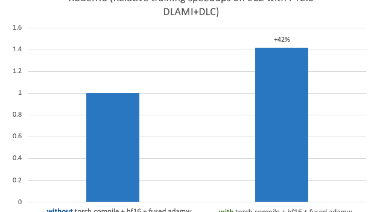


 Paul Hargis has focused his efforts on machine learning at several companies, including AWS, Amazon, and Hortonworks. He enjoys building technology solutions and teaching people how to leverage them. Paul likes to help customers expand their machine learning initiatives to solve real-world problems. Prior to his role at AWS, he was lead architect for Amazon Exports and Expansions, helping
  Mecit Gungor is an AI/ML Specialist Solution Architect at AWS helping customers design and build AI/ML solutions at scale. He covers a wide range of AI/ML use cases for Telecommunication customers and currently focuses on Generative AI, LLMs, and training and inference optimization. He can often be found hiking in the wilderness or playing board games with his friends in his free time.
 Tony Chen is a Machine Learning Solutions Architect at AWS, helping customers design scalable and robust machine learning capabilities in the cloud. As a former data scientist and data engineer, he leverages his experience to help tackle some of the most challenging problems organizations face with operationalizing machine learning.
 Sovik Kumar Nath is an AI/ML solution architect with AWS. He has extensive experience in end-to-end designs and solutions for machine learning; business analytics within financial, operational, and marketing analytics; healthcare; supply chain; and IoT. Outside work, Sovik enjoys traveling and watching movies.
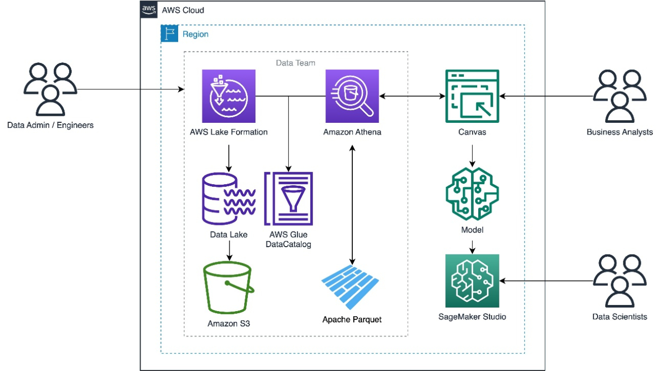


 Gopi Mudiyala is a Senior Technical Account Manager at AWS. He helps customers in the Financial Services industry with their operations in AWS. As a machine learning enthusiast, Gopi works to help customers succeed in their ML journey. In his spare time, he likes to play badminton, spend time with family, and travel.
 Hariharan Suresh is a Senior Solutions Architect at AWS. He is passionate about databases, machine learning, and designing innovative solutions. Prior to joining AWS, Hariharan was a product architect, core banking implementation specialist, and developer, and worked with BFSI organizations for over 11 years. Outside of technology, he enjoys paragliding and cycling.
 Jas Singh is a Senior Solutions Architect helping public sector customers achieve their business outcomes through architecting and implementing innovative and resilient solutions at scale. Jas has over 20 years of experience in designing and implementing mission-critical applications and holds a master’s degree in computer science from Baylor University.
 Raviteja Yelamanchili is an Enterprise Solutions Architect with Amazon Web Services based in New York. He works with large financial services enterprise customers to design and deploy highly secure, scalable, reliable, and cost-effective applications on the cloud. He brings over 11 years of risk management, technology consulting, data analytics, and machine learning experience. When he is not helping customers, he enjoys traveling and playing PS5.
 Iaroslav Shcherbatyi is a Machine Learning Engineer at AWS. He works mainly on improvements to the Amazon SageMaker platform and helping customers best use its features. In his spare time, he likes to go to gym, do outdoor sports such as ice skating or hiking, and to catch up on new AI research.