Ariadna Sanchez, a scientist who works in polyglot text to speech, draws on her musical background to help find novel solutions.Read More
Power recommendations and search using an IMDb knowledge graph – Part 2
This three-part series demonstrates how to use graph neural networks (GNNs) and Amazon Neptune to generate movie recommendations using the IMDb and Box Office Mojo Movies/TV/OTT licensable data package, which provides a wide range of entertainment metadata, including over 1 billion user ratings; credits for more than 11 million cast and crew members; 9 million movie, TV, and entertainment titles; and global box office reporting data from more than 60 countries. Many AWS media and entertainment customers license IMDb data through AWS Data Exchange to improve content discovery and increase customer engagement and retention.
In Part 1, we discussed the applications of GNNs, and how to transform and prepare our IMDb data for querying. In this post, we discuss the process of using Neptune to generate embeddings used to conduct our out-of-catalog search in Part 3 . We also go over Amazon Neptune ML, the machine learning (ML) feature of Neptune, and the code we use in our development process. In Part 3 , we walk through how to apply our knowledge graph embeddings to an out-of-catalog search use case.
Solution overview
Large connected datasets often contain valuable information that can be hard to extract using queries based on human intuition alone. ML techniques can help find hidden correlations in graphs with billions of relationships. These correlations can be helpful for recommending products, predicting credit worthiness, identifying fraud, and many other use cases.
Neptune ML makes it possible to build and train useful ML models on large graphs in hours instead of weeks. To accomplish this, Neptune ML uses GNN technology powered by Amazon SageMaker and the Deep Graph Library (DGL) (which is open-source). GNNs are an emerging field in artificial intelligence (for an example, see A Comprehensive Survey on Graph Neural Networks). For a hands-on tutorial about using GNNs with the DGL, see Learning graph neural networks with Deep Graph Library.
In this post, we show how to use Neptune in our pipeline to generate embeddings.
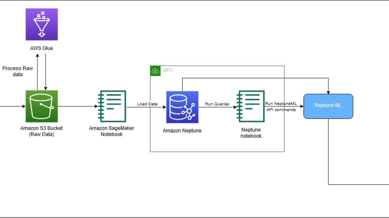
The following diagram depicts the overall flow of IMDb data from download to embedding generation.

We use the following AWS services to implement the solution:
- AWS CloudFormation
- Neptune ML
- SageMaker notebooks
- Amazon Simple Storage Service (Amazon S3).
In this post, we walk you through the following high-level steps:
- Set up environment variables
- Create an export job.
- Create a data processing job.
- Submit a training job.
- Download embeddings.
Code for Neptune ML commands
We use the following commands as part of implementing this solution:
We use neptune_ml export to check the status or start a Neptune ML export process, and neptune_ml training to start and check the status of a Neptune ML model training job.
For more information about these and other commands, refer to Using Neptune workbench magics in your notebooks.
Prerequisites
To follow along with this post, you should have the following:
- An AWS account
- Familiarity with SageMaker, Amazon S3, and AWS CloudFormation
- Graph data loaded into the Neptune cluster (see Part 1 <link to blog 1> for more information)
Set up environment variables
Before we begin, you’ll need to set up your environment by setting the following variables: s3_bucket_uri and processed_folder. s3_bucket_uri is the name of the bucket used in Part 1 and processed_folder is the Amazon S3 location for the output from the export job .
Create an export job
In Part 1, we created a SageMaker notebook and export service to export our data from the Neptune DB cluster to Amazon S3 in the required format.
Now that our data is loaded and the export service is created, we need to create an export job start it. To do this, we use NeptuneExportApiUri and create parameters for the export job. In the following code, we use the variables expo and export_params. Set expo to your NeptuneExportApiUri value, which you can find on the Outputs tab of your CloudFormation stack. For export_params, we use the endpoint of your Neptune cluster and provide the value for outputS3path, which is the Amazon S3 location for the output from the export job.
To submit the export job use the following command:
To check the status of the export job use the following command:
After your job is complete, set the processed_folder variable to provide the Amazon S3 location of the processed results:
Create a data processing job
Now that the export is done, we create a data processing job to prepare the data for the Neptune ML training process. This can be done a few different ways. For this step, you can change the job_name and modelType variables, but all other parameters must remain the same. The main portion of this code is the modelType parameter, which can either be heterogeneous graph models (heterogeneous) or knowledge graphs (kge).
The export job also includes training-data-configuration.json. Use this file to add or remove any nodes or edges that you don’t want to provide for training (for example, if you want to predict the link between two nodes, you can remove that link in this configuration file). For this blog post we use the original configuration file. For additional information, see Editing a training configuration file.
Create your data processing job with the following code:
To check the status of the export job use the following command:
Submit a training job
After the processing job is complete, we can begin our training job, which is where we create our embeddings. We recommend an instance type of ml.m5.24xlarge, but you can change this to suit your computing needs. See the following code:
We print the training_results variable to get the ID for the training job. Use the following command to check the status of your job:
%neptune_ml training status --job-id {training_results['id']} --store-to training_status_results
Download embeddings
After your training job is complete, the last step is to download your raw embeddings. The following steps show you how to download embeddings created by using KGE (you can use the same process for RGCN).
In the following code, we use neptune_ml.get_mapping() and get_embeddings() to download the mapping file (mapping.info) and the raw embeddings file (entity.npy). Then we need to map the appropriate embeddings to their corresponding IDs.
To download RGCNs, follow the same process with a new training job name by processing the data with the modelType parameter set to heterogeneous, then training your model with the modelName parameter set to rgcn see here for more details. Once that is finished, call the get_mapping and get_embeddings functions to download your new mapping.info and entity.npy files. After you have the entity and mapping files, the process to create the CSV file is identical.
Finally, upload your embeddings to your desired Amazon S3 location:
Make sure you remember this S3 location, you will need to use it in Part 3.
Clean up
When you’re done using the solution, be sure to clean up any resources to avoid ongoing charges.
Conclusion
In this post, we discussed how to use Neptune ML to train GNN embeddings from IMDb data.
Some related applications of knowledge graph embeddings are concepts like out-of-catalog search, content recommendations, targeted advertising, predicting missing links, general search, and cohort analysis. Out of catalog search is the process of searching for content that you don’t own, and finding or recommending content that is in your catalog that is as close to what the user searched as possible. We dive deeper into out-of-catalog search in Part 3.
About the Authors
 Matthew Rhodes is a Data Scientist I working in the Amazon ML Solutions Lab. He specializes in building Machine Learning pipelines that involve concepts such as Natural Language Processing and Computer Vision.
 Divya Bhargavi is a Data Scientist and Media and Entertainment Vertical Lead at the Amazon ML Solutions Lab, where she solves high-value business problems for AWS customers using Machine Learning. She works on image/video understanding, knowledge graph recommendation systems, predictive advertising use cases.
 Gaurav Rele is a Data Scientist at the Amazon ML Solution Lab, where he works with AWS customers across different verticals to accelerate their use of machine learning and AWS Cloud services to solve their business challenges.
 Karan Sindwani is a Data Scientist at Amazon ML Solutions Lab, where he builds and deploys deep learning models. He specializes in the area of computer vision. In his spare time, he enjoys hiking.
 Soji Adeshina is an Applied Scientist at AWS where he develops graph neural network-based models for machine learning on graphs tasks with applications to fraud & abuse, knowledge graphs, recommender systems, and life sciences. In his spare time, he enjoys reading and cooking.
 Vidya Sagar Ravipati is a Manager at the Amazon ML Solutions Lab, where he leverages his vast experience in large-scale distributed systems and his passion for machine learning to help AWS customers across different industry verticals accelerate their AI and cloud adoption.
Power recommendation and search using an IMDb knowledge graph – Part 1
The IMDb and Box Office Mojo Movies/TV/OTT licensable data package provides a wide range of entertainment metadata, including over 1 billion user ratings; credits for more than 11 million cast and crew members; 9 million movie, TV, and entertainment titles; and global box office reporting data from more than 60 countries. Many AWS media and entertainment customers license IMDb data through AWS Data Exchange to improve content discovery and increase customer engagement and retention.
In this three-part series, we demonstrate how to transform and prepare IMDb data to power out-of-catalog search for your media and entertainment use cases. In this post, we discuss how to prepare IMDb data and load the data into Amazon Neptune for querying. In Part 2, we discuss how to use Amazon Neptune ML to train graph neural network (GNN) embeddings from the IMDb graph. In Part 3, we walk through a demo application out-of-catalog search that is powered by the GNN embeddings.
Solution overview
In this series, we use the IMDb and Box Office Mojo Movies/TV/OTT licensed data package to show how you can built your own applications using graphs.
This licensable data package consists of JSON files with IMDb metadata for more than 9 million titles (including movies, TV and OTT shows, and video games) and credits for more than 11 million cast, crew, and entertainment professionals. IMDb’s metadata package also includes over 1 billion user ratings, as well as plots, genres, categorized keywords, posters, credits, and more.
IMDb delivers data through AWS Data Exchange, which makes it incredibly simple for you to access data to power your entertainment experiences and seamlessly integrate with other AWS services. IMDb licenses data to a wide range of media and entertainment customers, including pay TV, direct-to-consumer, and streaming operators, to improve content discovery and increase customer engagement and retention. Licensing customers also use IMDb data to enhance in-catalog and out-of-catalog title search and power relevant recommendations.
We use the following services as part of this solution:
- AWS Lambda
- Amazon Neptune
- Amazon Neptune ML
- Amazon OpenSearch Service
- AWS Glue
- Amazon SageMaker notebooks
- Amazon SageMaker Processing
- Amazon SageMaker Training
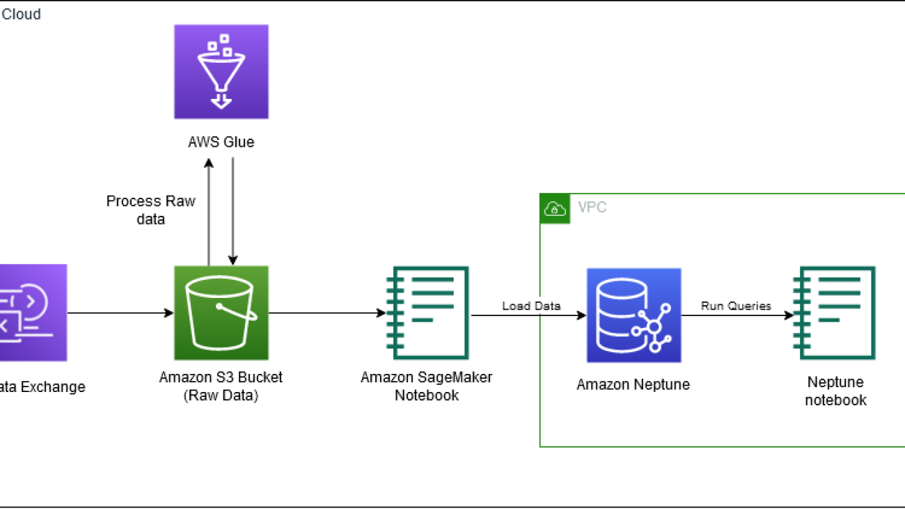
The following diagram depicts the workflow for part 1 of the 3 part blog series.

In this post, we walk through the following high-level steps:
- Provision Neptune resources with AWS CloudFormation.
- Access the IMDb data from AWS Data Exchange.
- Clone the GitHub repo.
- Process the data in Neptune Gremlin format.
- Load the data into a Neptune cluster.
- Query the data using Gremlin Query Language.
Prerequisites
The IMDb data used in this post requires an IMDb content license and paid subscription to the IMDb and Box Office Mojo Movies/TV/OTT licensing package in AWS Data Exchange. To inquire about a license and access sample data, visit developer.imdb.com.
Additionally, to follow along with this post, you should have an AWS account and familiarity with Neptune, the Gremlin query language, and SageMaker.
Provision Neptune resources with AWS CloudFormation
Now that you’ve seen the structure of the solution, you can deploy it into your account to run an example workflow.
You can launch the stack in AWS Region us-east-1 on the AWS CloudFormation console by choosing Launch Stack:
![]()
To launch the stack in a different Region, refer to Using the Neptune ML AWS CloudFormation template to get started quickly in a new DB cluster.
The following screenshot shows the stack parameters to provide.

Stack creation takes approximately 20 minutes. You can monitor the progress on the AWS CloudFormation console.
When the stack is complete, you’re now ready to process the IMDb data. On the Outputs tab for the stack, note the values for NeptuneExportApiUri and NeptuneLoadFromS3IAMRoleArn. Then proceed to the following steps to gain access to the IMDb dataset.
Access the IMDb data
IMDb publishes its dataset once a day on AWS Data Exchange. To use the IMDb data, you first subscribe to the data in AWS Data Exchange, then you can export the data to Amazon Simple Storage Service (Amazon S3). Complete the following steps:
- On the AWS Data Exchange console, choose Browse catalog in the navigation pane.
- In the search field, enter
IMDb. - Subscribe to either IMDb and Box Office Mojo Movie/TV/OTT Data (SAMPLE) or IMDb and Box Office Mojo Movie/TV/OTT Data.
- Complete the steps in the following workshop to export the IMDb data from AWS Data Exchange to Amazon S3.
Clone the GitHub repository
Complete the following steps:
- Open the SageMaker instance that you created from the CloudFormation template.
- Clone the GitHub repository.
Process IMDb data in Neptune Gremlin format
To add the data into Amazon Neptune, we process the data in Neptune gremlin format. From the GitHub repository, we run process_imdb_data.py to process the files. The script creates the CSVs to load the data into Neptune. Upload the data to an S3 bucket and note the S3 URI location.
Note that for this post, we filter the dataset to include only movies. You need either an AWS Glue job or Amazon EMR to process the full data.
To process the IMDb data using AWS Glue, complete the following steps:
- On the AWS Glue console, in the navigation pane, choose Jobs.
- On the Jobs page, choose Spark script editor.
- Under Options, choose Upload and edit existing script and upload the
1_process_imdb_data.pyfile. - Choose Create.
- On the editor page, choose Job Details.
- On the Job Details page, add the following options:
- For Name, enter
imdb-graph-processor. - For Description, enter
processing IMDb dataset and convert to Neptune Gremlin Format. - For IAM role, use an existing AWS Glue role or create an IAM role for AWS Glue. Make sure you give permission to your Amazon S3 location for the raw data and output data path.
- For Worker type, choose G 2X.
- For Requested number of workers, enter 20.
- For Name, enter
- Expand Advanced properties.
- Under Job Parameters, choose Add new parameter and enter the following key value pair:
- For the key, enter
--output_bucket_path. - For the value, enter the S3 path where you want to save the files. This path is also used to load the data into the Neptune cluster.
- For the key, enter
- To add another parameter, choose Add new parameter and enter the following key value pair:
- For the key, enter
--raw_data_path. - For the value, enter the S3 path where the raw data is stored.
- For the key, enter
- Choose Save and then choose Run.
This job takes about 2.5 hours to complete.
The following table provide details about the nodes for the graph data model.
| Description | Label |
| Principal cast members | Person |
| Long format movie | Movie |
| Genre of movies | Genre |
| Keyword descriptions of movies | Keyword |
| Shooting locations of movies | Place |
| Ratings for movies | rating |
| Awards event where movie received an award | awards |
Similarly, the following table shows some of the edges included in the graph. There will be in total 24 edge types.
| Description | Label | From | To |
| Movies an actress has acted in | casted-by-actress | Movie | Person |
| Movies an actor has acted in | casted-by-actor | Movie | Person |
| Keywords in a movie by character | described-by-character-keyword | Movie | keyword |
| Genre of a movie | is-genre | Movie | Genre |
| Place where the movie was shot | Filmed-at | Movie | Place |
| Composer of a movie | Crewed-by-composer | Movie | Person |
| award nomination | Nominated_for | Movie | Awards |
| award winner | Has_won | Movie | Awards |
Load the data into a Neptune cluster
In the repo, navigate to the graph_creation folder and run the 2_load.ipynb. To load the data to Neptune, use the %load command in the notebook, and provide your AWS Identity and Access Management (IAM) role ARN and Amazon S3 location of your processed data.
The following screen shot shows the output of the command.

Note that the data load takes about 1.5 hours to complete. To check the status of the load, use the following command:
When the load is complete, the status displays LOAD_COMPLETED, as shown in the following screenshot.

All the data is now loaded into graphs, and you can start querying the graph.

Fig: Sample Knowledge graph representation of movies in IMDb dataset. Movies “Saving Private Ryan” and “Bridge of Spies” have common connections like actor and director as well as indirect connections through movies like “The Catcher was a Spy” in the graph network.
Query the data using Gremlin
To access the graph in Neptune, we use the Gremlin query language. For more information, refer to Querying a Neptune Graph.
The graph consists of a rich set of information that can be queried directly using Gremlin. In this section, we show a few examples of questions that you can answer with the graph data. In the repo, navigate to the graph_creation folder and run the 3_queries.ipynb notebook. The following section goes over all the queries from the notebook.
Worldwide gross of movies that have been shot in New Zealand, with minimum 7.5 rating
The following query returns the worldwide gross of movies filmed in New Zealand, with a minimum rating of 7.5:
The following screenshot shows the query results.

Top 50 movies that belong to action and drama genres and have Oscar-winning actors
In the following example, we want to find the top 50 movies in two different genres (action and drama) with Oscar-winning actors. We can do this by using three different queries and merging the information using Pandas:
The following screenshot shows our results.

Top movies that have common keywords “tattoo” and “assassin”
The following query returns movies with keywords “tattoo” and “assassin”:
The following screenshot shows our results.

Movies that have common actors
In the following query, we find movies that have Leonardo DiCaprio and Tom Hanks:
We get the following results.

Conclusion
In this post, we showed you the power of the IMDb and Box Office Mojo Movies/TV/OTT dataset and how you can use it in various use cases by converting the data into a graph using Gremlin queries. In Part 2 of this series, we show you how to create graph neural network models on this data that can be used for downstream tasks.
For more information about Neptune and Gremlin, refer to Amazon Neptune Resources for additional blog posts and videos.
About the Authors
Gaurav Rele is a Data Scientist at the Amazon ML Solution Lab, where he works with AWS customers across different verticals to accelerate their use of machine learning and AWS Cloud services to solve their business challenges.
Matthew Rhodes is a Data Scientist I working in the Amazon ML Solutions Lab. He specializes in building Machine Learning pipelines that involve concepts such as Natural Language Processing and Computer Vision.
Divya Bhargavi is a Data Scientist and Media and Entertainment Vertical Lead at the Amazon ML Solutions Lab, where she solves high-value business problems for AWS customers using Machine Learning. She works on image/video understanding, knowledge graph recommendation systems, predictive advertising use cases.
Karan Sindwani is a Data Scientist at Amazon ML Solutions Lab, where he builds and deploys deep learning models. He specializes in the area of computer vision. In his spare time, he enjoys hiking.
Soji Adeshina is an Applied Scientist at AWS where he develops graph neural network-based models for machine learning on graphs tasks with applications to fraud & abuse, knowledge graphs, recommender systems, and life sciences. In his spare time, he enjoys reading and cooking.
Vidya Sagar Ravipati is a Manager at the Amazon ML Solutions Lab, where he leverages his vast experience in large-scale distributed systems and his passion for machine learning to help AWS customers across different industry verticals accelerate their AI and cloud adoption.
Accelerate the investment process with AWS Low Code-No Code services
The last few years have seen a tremendous paradigm shift in how institutional asset managers source and integrate multiple data sources into their investment process. With frequent shifts in risk correlations, unexpected sources of volatility, and increasing competition from passive strategies, asset managers are employing a broader set of third-party data sources to gain a competitive edge and improve risk-adjusted returns. However, the process of extracting benefits from multiple data sources can be extremely challenging. Asset managers’ data engineering teams are overloaded with data acquisition and preprocessing, while data science teams are mining data for investment insights.
Third-party or alternative data refers to data used in the investment process, sourced outside of the traditional market data providers. Institutional investors are frequently augmenting their traditional data sources with third-party or alternative data to gain an edge in their investment process. Typically cited examples include, but are not limited to, satellite imaging, credit card data, and social media sentiment. Fund managers invest nearly $3 billion annually in external datasets, with yearly spend growing by 20–30 percent.
With the exponential growth of available third-party and alternative datasets, the ability to quickly analyze whether a new dataset adds new investment insights is a competitive differentiator in the investment management industry. AWS no-code low-code (LCNC) data and AI services enable nontechnical teams to perform the initial data screening, prioritize data onboarding, accelerate time-to-insights, and free valuable technical resources—creating an enduring competitive advantage.
In this blog post, we discuss how, as an institutional asset manager, you can leverage AWS LCNC data and AI services to scale the initial data analysis and prioritization process beyond technical teams and accelerate your decision-making. With AWS LCNC services, you are able to quickly subscribe to and evaluate diverse third-party datasets, preprocess data, and check their predictive power using machine learning (ML) models without writing a single piece of code.
Solution overview
Our use case is to analyze the stock price predictive power of an external dataset and identify its feature importance—which fields most impact the stock price performance. This serves as a first-pass test to identify which of the multiple fields in a dataset should be more closely evaluated using traditional quantitative methodologies to fit with your investment process. This type of first-pass test can be done quickly by analysts, saving time and letting you more quickly prioritize dataset onboarding. Also, while we are using stock price as our target example, other metrics such as profitability, valuation ratios, or trading volumes could also be used. All datasets used for this use case are published in AWS Data Exchange.
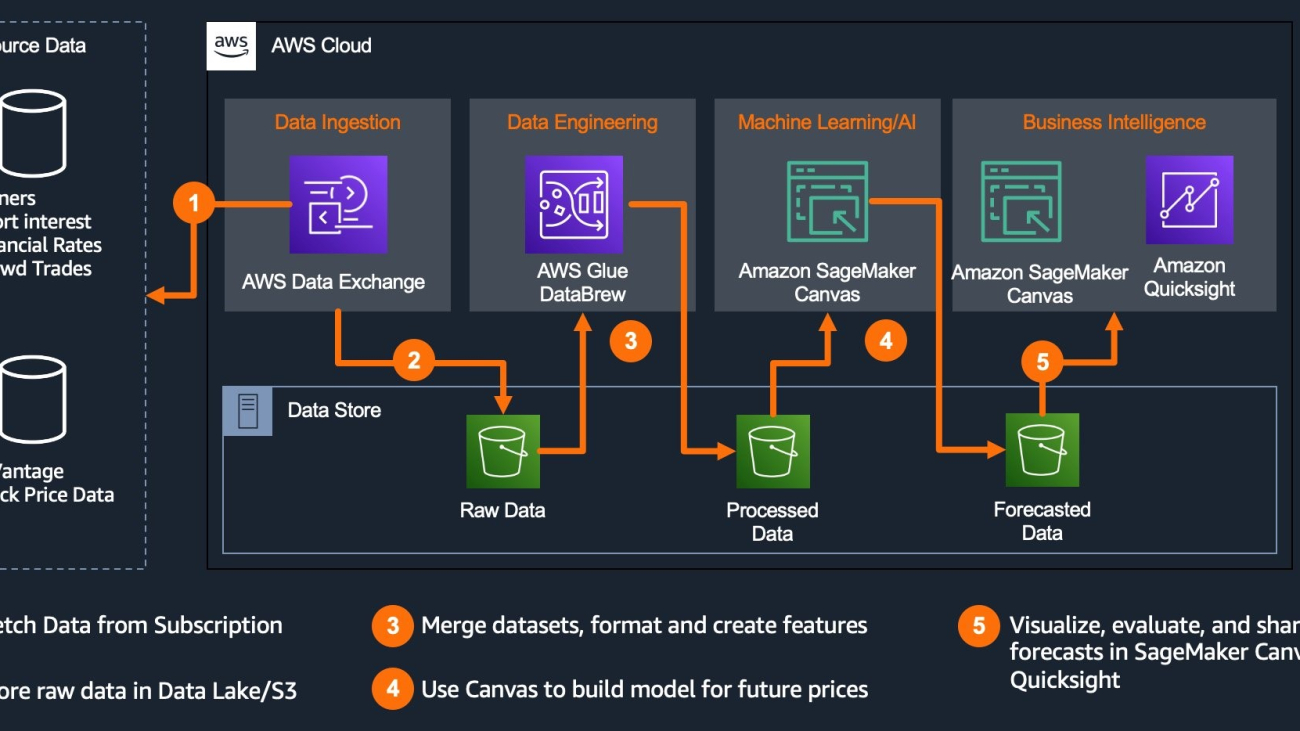
The following diagram explains the end-to-end architecture and the AWS LCNC services used to drive the decisions:

Our solution consists of the following steps and solutions:
- Data ingestion: AWS Data Exchange for subscribing to the published alternative datasets and downloading them on to Amazon Simple Storage Service (Amazon S3) bucket.
- Data engineering: AWS Glue DataBrew for data engineering and transformation of the data stored in Amazon S3.
- Machine learning: Amazon SageMaker Canvas for building a time series forecasting model for prediction and identifying the impact of data on the forecast.
- Business intelligence: Amazon QuickSight or Amazon SageMaker Canvas to review feature importance to the forecast for decision-making.
Data ingestion
AWS Data Exchange makes it easy to find, subscribe to, and use third-party data in the cloud. You can browse through the AWS Data Exchange catalog and find data products that are relevant to your business and subscribe to the data from the providers without any further processing, and no need for an ETL process. Note that many providers offer free initial subscriptions, which allow you to analyze their data without having to first incur upfront costs.
For this use case, search and subscribe to the below datasets in AWS Data Exchange:
- 20 Years of End-of-Day Stock Data for Top 10 US Companies by Market Cap published by Alpha Vantage. This free dataset contains 20 years of historical data for the top 10 US stocks by market capitalization as of September 5, 2020. The dataset contains the following 10 symbols—AAPL: Apple Inc.; AMZN: Amazon.com, Inc.; BRK-A: Berkshire Hathaway Inc. (Class A); FB: Facebook, Inc.; GOOG: Alphabet Inc.; JNJ: Johnson & Johnson; MA: Mastercard Incorporated; MSFT: Microsoft Corporation V: Visa Inc.; and WMT: Walmart Inc.
- Key data fields include
- Open: as-traded opening price for the day
- High: as-traded high price for the day
- Low: as-traded low price for the day
- Close: as-traded close price for the day
- Volume: trading volume for the day
- Adjusted Close: split and dividend-adjusted closing price of the day
- Split Ratio: ratio of new to old number of shares on the effective date
- Dividend: cash dividend payout amount
- S3 Short Interest and Securities Finance Data published by S3 partners. This dataset contains the following fields:
| Field | Description |
| Business Date | Effective date for the rate |
| Security IDs | Security identifiers contain Sedol, ISIN, FIGI, Ticker, Bloomberg ID |
| Name | Security Name |
| Offer Rate | Market composite financing fee paid for existing short positions |
| Bid Rate | Market composite lending fee earned for existing shares on loan by long holders |
| Last Rate | Market composite lending fee earned for incremental shares loaned on that date (spot rate) |
| Crowding | The momentum indicator measures daily shorting and covering events relative to the market float |
| Short Interest | Real-time short interest expressed in number of shares |
| ShortInterestNotional | ShortInterest * Price (USD) |
| ShortInterestPct | Real-time short interest expressed as a percentage of equity float |
| S3Float | The number of tradable shares including synthetic longs created by short selling |
| S3SIPctFloat | Real-time short interest projection divided by the S3 float |
| IndicativeAvailability | S3 projected available lendable quantity |
| Utilization | Real-time short interest divided by total lendable supply |
| DaystoCover10Day | It is a liquidity measure = short interest / 10-day average ADTV |
| DaystoCover30Day | It is a liquidity measure = short interest / 30-day average ADTV |
| DaystoCover90Day | It is a liquidity measure = short interest / 90-day average ADTV |
| Original SI | Point in time short interest |
To get the data, you will first search for the dataset in AWS Data Exchange and subscribe to the dataset:

Once the publisher of the datasets approves your subscription requests, you will have the datasets available for you to download to your S3 bucket:

Select Add auto-export job destination, provide the details of the S3 bucket, and download the dataset:

Repeat the steps to get the Alpha Vantage dataset. Once completed, you will have both datasets in your S3 bucket.
Data engineering
Once the dataset is in your S3 buckets, you can use AWS Glue DataBrew to transform the data. AWS Glue DataBrew offers over 350 pre-built transformations to automate data preparation tasks (such as filtering anomalies, standardizing formats, and correcting invalid values) that would otherwise require days or weeks of writing hand-coded transformations.
To create a consolidated curated dataset for forecasting in AWS DataBrew, perform the below steps. For detailed information, please refer to this blog.
- Create the DataBrew datasets.
- Load DataBrew datasets into DataBrew projects.
- Build the DataBrew recipes.
- Run the DataBrew jobs.
Create DataBrew Datasets: In AWS Glue DataBrew, a dataset represents data that is uploaded from the S3 bucket. We will create two DataBrew datasets—for both end-of-day stock price and S3 short interest. When you create your dataset, you enter the S3 connection details only once. From that point, DataBrew can access the underlying data for you.
Load the DataBrew datasets into DataBrew projects: In AWS Glue DataBrew, a project is the centerpiece of your data analysis and transformation efforts. A DataBrew project brings together the DataBrew datasets and enables you to develop a data transformation (DataBrew recipe). Here again, we will create two DataBrew projects, for end-of-day stock price and S3 short interest.

Build the DataBrew recipes: In DataBrew, a recipe is a set of data transformation steps. You can apply these steps to your dataset. For the use case, we will build two transformations. The first one will change the format of the end-of-day stock price timestamp column so that the dataset can be joined to the S3 short interest:

The second transformation curates the data, and its last step ensures we join the datasets into a single curated dataset. For more details on building data transformation recipes, refer to this blog.

DataBrew jobs: After the creation of the DataBrew recipes, you can run first the end-of-day stock price DataBrew job followed by the S3 short interest recipe. Refer to this blog to create a single consolidated dataset. Save the final curated dataset into an S3 bucket.
The end-to-end data engineering workflow will look like this:

Machine learning
With the curated dataset created post-data engineering, you can use Amazon SageMaker Canvas to build your forecasting model and analyze the impact of features on the forecast. Amazon SageMaker Canvas provides business users with a visual point-and-click interface that allows them to build models and generate accurate ML predictions on their own—without requiring any ML experience or having to write a single line of code.
To build a time series forecasting model in Amazon SageMaker Canvas, follow the below steps. For detailed information, refer to this blog:
- Select the curated dataset in SageMaker Canvas.
- Build the time series forecasting model.
- Analyze the results and feature importance.
Build the time series forecasting model: Once you have selected the dataset, select the target column to be predicted. In our case, this will be the close price of the stock ticker. SageMaker Canvas automatically detects this is a time series forecasting problem statement.

You will have to configure the model as follows for time series forecasting. For item ID, select the stock ticker name. Remember, our dataset has stock ticker prices for the top 10 stocks. Select the timestamp column for the time stamp, and finally, enter the number of days you want to forecast in the future [Forecast Horizon].

Now you are ready to build the model. SageMaker Canvas provides two options to build the model: Quick Build and Standard Build. In our case, we will use “Standard Build”.

Standard Build takes approximately three hours to build the model and uses Amazon Forecast, a time series forecasting service based on ML as the underlying forecasting engine. Forecast creates highly accurate forecasts through model ensembling of traditional and deep learning models without requiring ML experience.

Once the model is built, you can now review the model performance (prediction accuracy) and feature importance. As can be seen from the figure below, the model identifies Crowding and DaysToCover10Day as the two top features driving forecast values. This is in line with our market intuition, as crowding is a momentum indicator measuring daily shorting and covering events, and near-term short interest is a liquidity measure, indicating how investors are positioned in a stock. Both momentum and liquidity can drive price volatility.

This result indicates that these two features (or fields) have a close relationship with stock price movements and can be prioritized higher for onboarding and further analysis.
Business intelligence
In the context of time series forecasting, the notion of backtesting refers to the process of assessing the accuracy of a forecasting method using existing historical data. The process is typically iterative and repeated over multiple dates present in the historical data.
As we already discussed, SageMaker Canvas uses Amazon Forecast as the engine for time-series forecasting. Forecast creates a backtest as a part of the model building process. You can now view the predictor details by signing in to Amazon Forecast. For deeper dive understanding on Model Explainability, refer to this blog.

Amazon Forecast provides additional details on predictor metrics like weighted absolute percentage error (WAPE), root mean square error (RMSE), mean absolute percentage error (MAPE), and mean absolute scaled error (MASE). You can export predictor quality scores from Amazon Forecast.

Amazon Forecast runs one backtest for the time series dataset provided. The backtest results are available for download using the Export backtest results button. Exported backtest results are downloaded to an S3 bucket.
We will now plot the backtest results in Amazon QuickSight. To visualize the backtest results in Amazon QuickSight, connect to the dataset in Amazon S3 from QuickSight and create a visualization.

Clean up
AWS services leveraged in this solution are managed and serverless in nature. SageMaker Canvas is designed to run long running ML training and will be always on. Ensure you explicitly log off SageMaker Canvas. Please refer to the docs for more details.
Conclusion
In this blog post, we discussed how, as an institutional asset manager, you can leverage AWS low-code no-code (LCNC) data and AI services to accelerate the evaluation of external datasets by offloading the initial dataset screening to nontechnical personnel. This first-pass analysis can be done quickly to help you decide which datasets should be prioritized for onboarding and further analysis.
We demonstrated step-by-step how a data analyst can acquire new third-party data through AWS Data Exchange , use AWS Glue DataBrew no-code ETL services to preprocess data and evaluate which features in a dataset have the most impact on the model’s forecast.
Once data is analysis-ready, an analyst uses SageMaker Canvas to build a predictive model, evaluate its fit and identify significant features. In our example, the model’s MAPE (.05) and WAPE (.045) indicated a good fit and showed “Crowding” and “DaysToCover10Day” as the signals in the dataset with the largest impact over the forecast. This analysis quantified what data most influenced the model and could therefore be prioritized for further investigation and potential inclusion into your alpha signals or risk management process. And just as importantly, explainability scores indicate what data plays relatively little role in determining the forecast and therefore can be a lower priority for further investigation.
To more quickly evaluate the ability of third-party financial data to support your investment process, review the Financial Services data sources available on AWS Data Exchange, and give DataBrew and Canvas a try today.
About the Authors
 Boris Litvin is Principal Solution Architect, responsible for Financial Services industry innovation. He is a former Quant and FinTech founder, passionate about systematic investing.
 Meenakshisundaram Thandavarayan is a Senior AI/ML specialist with AWS. He helps high-tech strategic accounts on their AI and ML journey. He is very passionate about data-driven AI.
 Camillo Anania is a Senior Startup Solutions Architect with AWS based in the UK. He is a passionate technologist helping startups of any size build and grow.
 Dan Sinnreich is a Sr. Product Manager with AWS, focused on empowering companies to make better decisions with ML. He formerly built portfolio analytics platforms and multi-asset class risk models for large institutional investors.
Automatically retrain neural networks with Renate
Today we announce the general availability of Renate, an open-source Python library for automatic model retraining. The library provides continual learning algorithms able to incrementally train a neural network as more data becomes available.
By open-sourcing Renate, we would like to create a venue where practitioners working on real-world machine learning systems and researchers interested in advancing the state of the art in automatic machine learning, continual learning, and lifelong learning come together. We believe that synergies between these two communities will generate new ideas in the machine learning research community and provide a tangible positive impact in real-world applications.
Model retraining and catastrophic forgetting
Training neural networks incrementally is not a simple task. In practice, data provided at different points in time is often sampled from different distributions. For example, in question-answering systems, the distribution of the topics in the questions can significantly vary over time. In classification systems, the addition of new categories may be required when the data is collected in different parts of the world. Fine-tuning the previously trained models with new data in these cases will lead to a phenomenon called “catastrophic forgetting.” There will be good performance on the most recent examples, but the quality of the predictions made for data collected in the past will degrade significantly. Moreover, the performance degradation will be even more severe when the retraining operation happens regularly (e.g., daily or weekly).
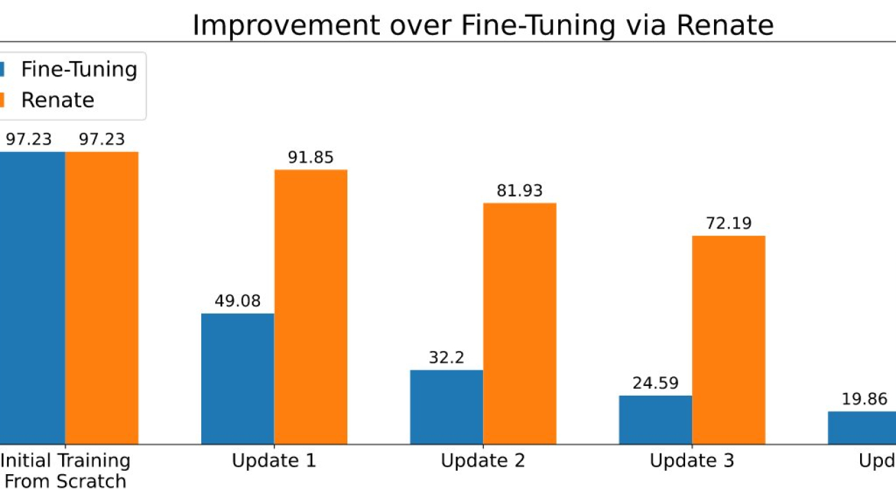
When storing a small chunk of data is possible, methods based on reusing old data during the retraining can partially alleviate the catastrophic forgetting problem. Several methods have been developed following this idea. Some of them store only the raw data, while more advanced ones also save additional metadata (e.g., the intermediate representation of the data points in memory). Storing a small amount of data (e.g., thousands of data points) and using them carefully led to the superior performance displayed in the figure below.

Bring your own model and dataset
When training neural network models, it may be necessary to change the network structure, the data transformation and other important details. While code changes are limited, it can become a complex task when these models are part of a large software library. To avoid these inconveniences, Renate offers customers the ability to define their models and datasets in predefined Python functions as part of a configuration file. This has the advantage of keeping the customers’ code clearly separate from the rest of the library and allow customers without any knowledge of the Renate’s internal structure to use the library effectively.
Moreover, all functions, including the model definition, are very flexible. In fact, the model definition function allows users to create neural networks from scratch following their own needs or to instantiate well-known models from open-source libraries like transformers or torchvision. It just requires adding the necessary dependencies to the requirements file.
A tutorial on how to write the configuration file is available at How to Write a Config File.
The benefit of hyperparameter optimization
As is often the case in machine learning, continual learning algorithms come with a number of hyperparameters. Its settings can make an important difference in the overall performance, and careful tuning can positively impact the predictive performance. When training a new model, Renate can enable hyperparameter optimization (HPO) using state-of-the-art algorithms like ASHA to exploit the ability to run multiple parallel jobs on Amazon SageMaker. An example of the outcomes is displayed in the figure below.
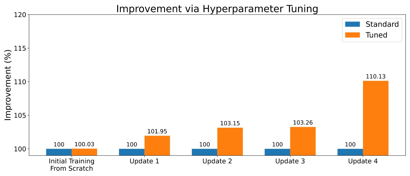
In order to enable HPO, the user will need to define the search space or use one of the default search spaces provided with the library. Refer to the example at Run a training job with HPO. Customers that are looking for a quicker retuning can also leverage the results of their previous tuning jobs by selecting algorithms with transfer learning functionalities. In this way, optimizers will be informed about which hyperparameters are performing well across different tuning jobs and will be able to focus on those, reducing the tuning time.
Run it in the cloud
Renate allows users to quickly transition from training models on a local machine for experimentation to train large-scale neural networks using SageMaker. In fact, running training jobs on a local machine is rather unusual, especially when training large-scale models. At the same time, being able to verify details and test the code locally can be extremely useful. To answer this need, Renate allows quick switching between the local machine and the SageMaker service just by changing a simple flag in the configuration file.
For example, when launching a tuning job, it is possible to run locally execute_tuning_job(..., backend='local') and quickly switch to SageMaker, changing the code as follows:
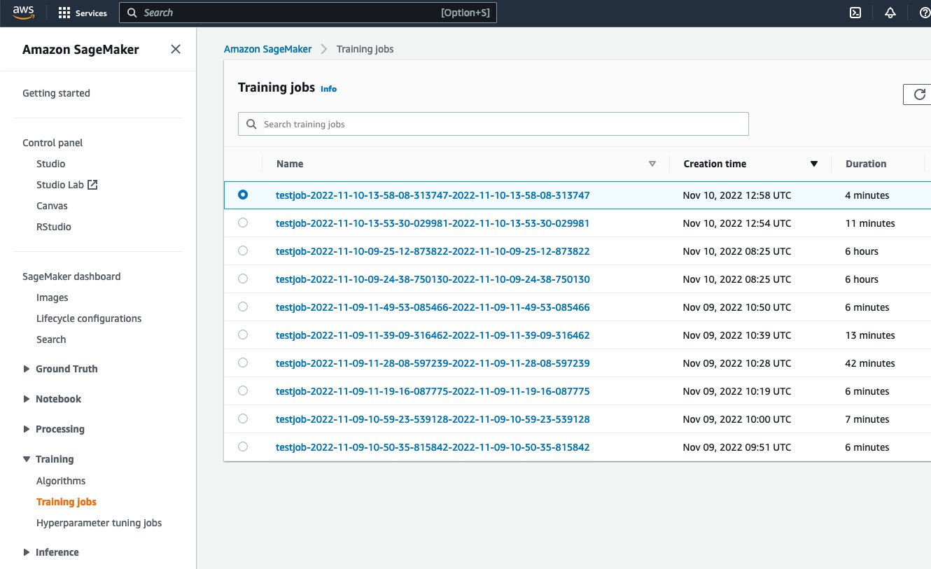
After running the script, it will be possible to see the job running from the SageMaker web interface:
It will also be possible to monitor the training job and read the logs in CloudWatch:
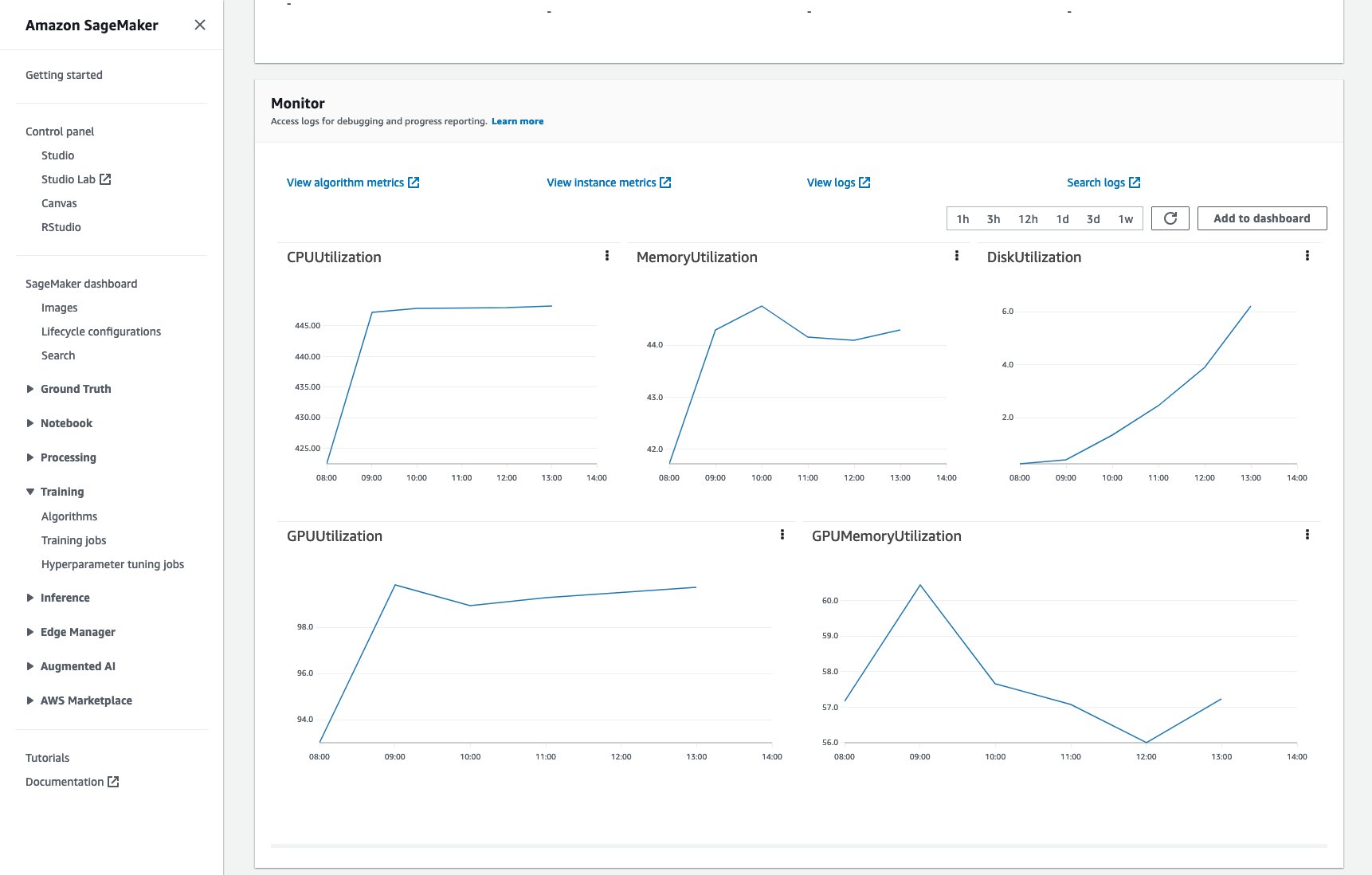
All of this without any additional code or effort.
A full example of running training jobs in the cloud is available at How to Run a Training Job.
Conclusion
In this post, we described the problems associated with retraining neural networks and the main benefits of the Renate library in the process. To learn more about the library, check out the GitHub repository, where you will find a high-level overview of the library and its algorithms, instructions for the installation, and examples that can help you to get you started.
We look forward to your contributions, feedback and discussing this further with everyone interested, and to seeing the library integrated into real-world retraining pipelines.
About the authors
 Giovanni Zappella is a Sr. Applied Scientist working on Long-term science at AWS Sagemaker. He currently works on continual learning, model monitoring and AutoML. Before that he worked on applications of multi-armed bandits for large-scale recommendations systems at Amazon Music.
 Martin Wistuba is an Applied Scientist in the Long-term science team at AWS Sagemaker. His research focuses on automatic machine learning.
 Lukas Balles is an Applied Scientist at AWS. He works on continual learning and topics relating to model monitoring.
 Cedric Archambeau is a Principal Applied Scientist at AWS and Fellow of the European Lab for Learning and Intelligent Systems.
Create Amazon SageMaker models using the PyTorch Model Zoo
Deploying high-quality, trained machine learning (ML) models to perform either batch or real-time inference is a critical piece of bringing value to customers. However, the ML experimentation process can be tedious—there are a lot of approaches requiring a significant amount of time to implement. That’s why pre-trained ML models like the ones provided in the PyTorch Model Zoo are so helpful. Amazon SageMaker provides a unified interface to experiment with different ML models, and the PyTorch Model Zoo allows us to easily swap our models in a standardized manner.
This blog post demonstrates how to perform ML inference using an object detection model from the PyTorch Model Zoo within SageMaker. Pre-trained ML models from the PyTorch Model Zoo are ready-made and can easily be used as part of ML applications. Setting up these ML models as a SageMaker endpoint or SageMaker Batch Transform job for online or offline inference is easy with the steps outlined in this blog post. We will use a Faster R-CNN object detection model to predict bounding boxes for pre-defined object classes.
We walk through an end-to-end example, from loading the Faster R-CNN object detection model weights, to saving them to an Amazon Simple Storage Service (Amazon S3) bucket, and to writing an entrypoint file and understanding the key parameters in the PyTorchModel API. Finally, we will deploy the ML model, perform inference on it using SageMaker Batch Transform, and inspect the ML model output and learn how to interpret the results. This solution can be applied to any other pre-trained model on the PyTorch Model Zoo. For a list of available models, see the PyTorch Model Zoo documentation.
Solution overview
This blog post will walk through the following steps. For a full working version of all steps, see create_pytorch_model_sagemaker.ipynb
- Step 1: Setup
- Step 2: Loading an ML model from PyTorch Model Zoo
- Step 3 Save and upload ML model artifacts to Amazon S3
- Step 4: Building ML model inference scripts
- Step 5: Launching a SageMaker batch transform job
- Step 6: Visualizing results
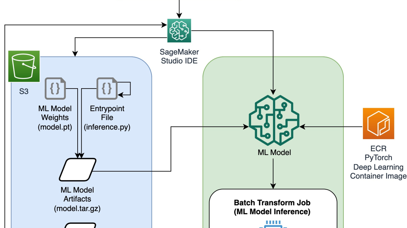
Architecture diagram

Directory structure
The code for this blog can be found in this GitHub repository. The codebase contains everything we need to build ML model artifacts, launch the transform job, and visualize results.
This is the workflow we use. All of the following steps will refer to modules in this structure.
The sagemaker_torch_model_zoo folder should contain inference.py as an entrypoint file, and create_pytorch_model_sagemaker.ipynb to load and save the model weights, create a SageMaker model object, and finally pass that into a SageMaker batch transform job. In order to bring your own ML models, change the paths in the Step 1: setup section of the notebook and load a new model in the Step 2: Loading an ML Model from the PyTorch Model Zoo section. The rest of the following steps below would remain the same.
Step 1: Setup
IAM roles
SageMaker performs operations on infrastructure that is managed by SageMaker. SageMaker can only perform actions permitted as defined in the notebook’s accompanying IAM execution role for SageMaker. For a more detailed documentation on creating IAM roles and managing IAM permissions, refer to the AWS SageMaker roles documentation. We can create a new role, or we could get the SageMaker (Studio) notebook’s default execution role by running the following lines of code:
The above code gets the SageMaker execution role for the notebook instance. This is the IAM role that we created for our SageMaker or SageMaker Studio notebook instance.
User configurable parameters
Here are all the configurable parameters needed for building and launching our SageMaker batch transform job:
Step 2: Loading an ML model from the PyTorch Model Zoo
Next, we specify an object detection model from the PyTorch Model Zoo and save its ML model weights. Typically, we save a PyTorch model using the .pt or .pth file extensions. The code snippet below downloads a pre-trained Faster R-CNN ResNet50 ML model from the PyTorch Model Zoo:
model = torchvision.models.detection.fasterrcnn_resnet50_fpn(pretrained=True)
SageMaker batch transform requires as an input some model weights, so we will save the pre-trained ML model as model.pt. If we want to load a custom model, we could save the model weights from another PyTorch model as model.pt instead.
Step 3: Save and upload ML model artifacts to Amazon S3
Since we will be using SageMaker for ML inference, we need to upload the model weights to an S3 bucket. We can do this using the following commands or by downloading and simply dragging and dropping the file directly into S3. The following commands will first compress the group of files within model.pt to a tarball and copy the model weights from our local machine to the S3 bucket.
Note: To run the following commands, you need to have the AWS Command Line Interface (AWS CLI) installed.
Next, we copy our input image over to S3. Below is the full S3 path for the image.
We can copy over this image to S3 with another aws s3 cp command.
Step 4: Building ML model inference scripts
Now we will go over our entrypoint file, inference.py module. We can deploy a PyTorch model trained outside of SageMaker using the PyTorchModel class. First, we instantiate the PyTorchModelZoo object. Then we will construct an inference.py entrypoint file to perform ML inference using SageMaker batch transform on sample data hosted in Amazon S3.
Understanding the PyTorchModel object
The PyTorchModel class within the SageMaker Python API allows us to perform ML inference using our downloaded model artifact.
To initiate the PyTorchModel class, we need to understand the following input parameters:
name: Model name; we recommend using either the model name + date time, or a random string + date time for uniqueness.model_data: The S3 URI of the packaged ML model artifact.entry_point: A user-defined Python file to be used by the inference Docker image to define handlers for incoming requests. The code defines model loading, input preprocessing, prediction logic, and output post-processing.framework_version: Needs to be set to version 1.2 or higher to enable automatic PyTorch model repackaging.source_dir: The directory of the entry_point file.role: An IAM role to make AWS service requests.image_uri: Use this Amazon ECR Docker container image as a base for the ML model compute environment.sagemaker_session: The SageMaker session.py_version: The Python version to be used
The following code snippet instantiates the PyTorchModel class to perform inference using the pre-trained PyTorch model:
Understanding the entrypoint file (inference.py)
The entry_point parameter points to a Python file named inference.py. This entrypoint defines model loading, input preprocessing, prediction logic, and output post-processing. It supplements the ML model serving code in the prebuilt PyTorch SageMaker Deep Learning Container image.
Inference.py will contain the following functions. In our example, we implement the model_fn, input_fn, predict_fn and output_fn functions to override the default PyTorch inference handler.
model_fn: Takes in a directory containing static model checkpoints in the inference image. Opens and loads the model from a specified path and returns a PyTorch model.input_fn: Takes in the payload of the incoming request (request_body) and the content type of an incoming request (request_content_type) as input. Handles data decoding. This function needs to be adjusted for what input the model is expecting.predict_fn: Calls a model on data deserialized in input_fn. Performs prediction on the deserialized object with the loaded ML model.output_fn: Serializes the prediction result into the desired response content type. Converts predictions obtained from the predict_fn function to JSON, CSV, or NPY formats.
Step 5: Launching a SageMaker batch transform job
For this example, we will obtain ML inference results through a SageMaker batch transform job. Batch transform jobs are most useful when we want to obtain inferences from datasets once, without the need for a persistent endpoint. We instantiate a sagemaker.transformer.Transformer object for creating and interacting with SageMaker batch transform jobs.
See the documentation for creating a batch transform job at CreateTransformJob.
Step 6: Visualizing tesults
Once the SageMaker batch transform job finishes, we can load the ML inference outputs from Amazon S3. For this, navigate to the AWS Management Console and search for Amazon SageMaker. On the left panel, under Inference, see Batch transform jobs.

After selecting Batch transform, see the webpage listing all SageMaker batch transform jobs. We can view the progress of our most recent job execution.

First, the job will have the status “InProgress.” Once it’s done, see the status change to Completed.

Once the status is marked as completed, we can click on the job to view the results. This webpage contains the job summary, including configurations of the job we just executed.

Under Output data configuration, we will see an S3 output path. This is where we will find our ML inference output.

Select the S3 output path and see an [image_name].[file_type].out file with our output data. Our output file will contain a list of mappings. Example output:
Next, we process this output file and visualize our predictions. Below we specify our confidence threshold. We get the list of classes from the COCO dataset object mapping. During inference, the model requires only the input tensors and returns the post-processed predictions as a List[Dict[Tensor]], one for each input image. The fields of the Dict are as follows, where N is the number of detections:
- boxes (FloatTensor[N, 4]): the predicted boxes in
[x1, y1, x2, y2]format, with0 <= x1 < x2 <= W and 0 <= y1 < y2 <= H, whereWis the width of the image andHis the height of the image - labels (
Int64Tensor[N]): the predicted labels for each detection - scores (
Tensor[N]): the prediction scores for each detection
For more details on the output, refer to the PyTorch Faster R-CNN FPN Documentation.
The model output contains bounding boxes with respective confidence scores. We can optimize displaying false positives by removing bounding boxes for which the model is not confident. The following code snippets process the predictions in the output file and draw bounding boxes on the predictions where the score is above our confidence threshold. We set the probability threshold, CONF_THRESH, to .75 for this example.
Finally, we visualize these mappings to understand our output.

Note: if the image doesn’t display in your notebook, please locate it in the directory tree on the left-hand side of JupyterLab and open it from there.
Running the example code
For a full working example, clone the code in the amazon-sagemaker-examples GitHub and run the cells in the create_pytorch_model_sagemaker.ipynb notebook.
Conclusion
In this blog post, we showcased an end-to-end example of performing ML inference using an object detection model from the PyTorch Model Zoo using SageMaker batch transform. We covered loading the Faster R-CNN object detection model weights, saving them to an S3 bucket, writing an entrypoint file, and understanding the key parameters in the PyTorchModel API. Finally, we deployed the model and performed ML model inference, visualized the model output, and learned how to interpret the results.
About the Authors
 Dipika Khullar is an ML Engineer in the Amazon ML Solutions Lab. She helps customers integrate ML solutions to solve their business problems. Most recently, she has built training and inference pipelines for media customers and predictive models for marketing.
 Marcelo Aberle is an ML Engineer in the AWS AI organization. He is leading MLOps efforts at the Amazon ML Solutions Lab, helping customers design and implement scalable ML systems. His mission is to guide customers on their enterprise ML journey and accelerate their ML path to production.
 Ninad Kulkarni is an Applied Scientist in the Amazon ML Solutions Lab. He helps customers adopt ML and AI by building solutions to address their business problems. Most recently, he has built predictive models for sport, automotive, and media customers.
 Yash Shah is a Science Manager in the Amazon ML Solutions Lab. He and his team of applied scientists and ML engineers work on a range of ML use cases from healthcare, sports, automotive, and manufacturing.
Controlling formality in machine translation
Transfer learning using limited contrastive data improves formality accuracy without compromising performance.Read More

New performance improvements in Amazon SageMaker model parallel library
Foundation models are large deep learning models trained on a vast quantity of data at scale. They can be further fine-tuned to perform a variety of downstream tasks and form the core backbone of enabling several AI applications. The most prominent category is large-language models (LLM), including auto-regressive models such as GPT variants trained to complete natural text. LLMs typically contain billions of parameters, making them rarely fit on one single accelerator, and require model parallelism techniques. Another category is diffusion models, notably Stable Diffusion, that has pushed AI image generation to an unprecedented milestone where remarkable visuals can be generated from a simple text description. Diffusion models are typically much smaller than LLMs and distributed training remains to play a critical role in facilitating development.
SageMaker model parallel (SMP) library is a large-model training solution available on Amazon SageMaker platform. It can be integrated with PyTorch models to easily apply a range of state-of-the-art large-model distributed training techniques to train at scale. Earlier this year, SMP launched sharded data parallelism, a distributed training technique powered by Amazon in-house MiCS technology under the hood. Sharded data parallel shards model parameters, gradients, and optimizer states across data-parallel workers. MiCS performs a number of optimizations including scale-aware partitioning to provide near-linear scalability. In Train gigantic models with near-linear scaling using sharded data parallelism, we shared that sharded data parallel in SMP achieved 39.7% speed up compared to DeepSpeed ZeRO-3 on a 30B parameter GPT-2 model with sequence length 2048.
To help our customers further minimize training costs and accelerate time-to-market, we are thrilled to introduce two new performance improvements in SageMaker model parallel — SMDDP Collectives and FlashAttention. SMDDP Collectives is the most performant collective library on AWS infrastructure for large model training offered by SageMaker distributed data parallel library. FlashAttention is introduced in Dao et al., which re-implements the attention mechanism in an IO-aware manner, reducing the memory bandwidth requirement and saving on attention speed and memory footprint. These two components collectively push our sharded data parallel technique to be 30.58% faster when training a 100B parameter GPT-NeoX model on 32 p4d.24xlarge instances. For customers who are already using sharded data parallel on supported models, no code changes are necessary to benefit from the performance boost offered by these latest features. Stability AI, the inventor of the Stable Diffusion family of models that showed unparalleled image generation abilities, chose to use SMP to build foundation models. With SMP, Stability AI achieved 163 TFLOPs per GPU for a 13B-parameter GPT-NeoX on 32 p4d.24xlarge instances, a 58% speed up compared to DeepSpeed. You can learn more about Stability AI’s mission and partnership with AWS in the talk of Stability AI CEO at AWS re:Invent 2022 or in this blog post.
“Our mission at Stability AI is to build the foundation to activate humanity’s potential through AI. To achieve this mission, we need to efficiently train open-source foundation models on hundreds of accelerated compute instances. We rely on SageMaker and its distributed training libraries to optimize performance and implement state-of-the-art strategies to shard models and data across our training cluster. These optimizations reduce our training costs, help us meet customer needs faster, and speed up the development of new models.”
— Emad Mostaque, Founder and CEO of Stability AI.
In this blog post, we’ll first present our latest performance improvements in the SageMaker model parallel library. Then, we’ll revisit how to train foundational models using sharded data parallel. Finally, we’ll benchmark performance of 13B, 50B, and 100B parameter auto-regressive models and wrap up with future work.
New performance improvements in SageMaker model parallel library
Starting from AWS Deep Learning Containers (DLC) PyTorch 1.12.1, SageMaker model parallel library v1.13 comes with the following two new components that are critical in improving training performance. They are currently available on ml.p4d.24xlarge instance with Elastic Fabric Adapter (EFA) enabled:
1. AWS-optimized AllGather from SMDDP Collectives
In sharded data parallel, since only a shard of the model state is present on a GPU, an AllGather collective is needed to gather the full set of parameters from across all GPUs in the sharding group during forward or backward pass computations. In the previous versions of SageMaker model parallel, we used NVIDIA Collective Communications Library (NCCL) for these collectives. However, NCCL is a general purpose collective communications library not designed for AWS infrastructure, which leads to sub-optimal performance even with EFA enabled.
Previously, we had developed the SMDDP Collectives library that provided an AWS-optimized implementation of the All-Reduce collective to speedup performance of pure data parallel training. To improve the performance of large model training with sharded data parallelism, we expanded the SMDDP Collectives library to include an optimized implementation of the AllGather collective. The key advantage of SMDDP Collectives AllGather is that it adopts an all-to-all-type communication pattern for inter-node communication, enabling our collective to have high-throughput and be less latency-sensitive. In addition, our AllGather collective offloads the communication-related processing to the CPU, thereby freeing up valuable GPU cycles for gradient computation, leading to significant performance improvement especially on large models.
2. FlashAttention
In modern transformer architecture, one of the largest sources of memory consumption is the activation footprint in the self-attention layer. This is because each attention head computes an SxS attention matrix for each input, where S is the sequence length, and this matrix goes through several operations, such as dropout, softmax, and matrix multiplication, with each intermediate output requiring memory space for use in back-propagation.
FlashAttention (Dao et al.) is a recent innovation from HazyResearch in Stanford that re-implements the self-attention mechanism in an I/O-aware manner. The main insight behind FlashAttention is that the self-attention mechanism is bottlenecked by memory bandwidth to and from GPU high bandwidth memory (HBM). This means that the self-attention layer can be computed in chunks across the sequence dimension, with each chunk going through the entire self-attention pipeline at a time. The intermediate results for a chunk are stored at the high-bandwidth SRAM, avoiding the expensive round-trip to the HBM for every iteration. Although a naive implementation would run into the issue of the cross-chunk dependency at the softmax layer, FlashAttention introduces a clever implementation that side-steps this dependency. Combined with re-computation in backward pass, FlashAttention results in substantial memory savings and performance improvement (25% faster training for GPT-NeoX 13B over 16 p4d nodes), due to avoidance of the HBM round-trip and storage of SxS matrices. You can find visuals and more explanations in HazyResearch’s FlashAttention repository.
Train foundation models at scale with SageMaker model parallel
To train foundation models with SMP powered by SMDDP Collectives, there’s no additional changes required in your sharded data parallel training jobs. If you’re new to using sharded data parallel, follow this complete tutorial notebook and blog post that will walk you through the entire process, from data processing, defining and submitting training jobs, to monitoring training logs. A ready-to-use training script for GPT-2 model can be found at train_gpt_simple.py. For training a different model type, you can follow the API document to learn about how to apply SMP APIs.
We highlight the key hyperparameters in the PyTorch Estimator of a sharded data parallel training job as below. The hyperparameter ddp_dist_backend in smp_options now has a new option, "auto" , as its default value. With "auto", SMP will use AWS-optimized AllGather for sharded data parallelism jobs and fall back to NCCL otherwise. You can refer to this document for supported configurations. If you want to run sharded data parallel in SMP specifically with NCCL as the communication backend of choice, you can set “ddp_dist_backend" to "nccl" in smp_options.
With the latest SMPv1.13 release, the sharded data parallel training technique supports FlashAttention for popular models including BERT, RoBERTa, GPT-2, GPT-J, GPT-Neo and GPT-NeoX out-of-the-box. This is enabled by passing tensor_parallelism=True during model creation without setting tensor_parallel_degree. You can find an example in the same training script train_gpt_simple.py .
Benchmarking performance
We benchmarked sharded data parallelism in the SageMaker model parallel library on three different scales of models to understand how the two new features, FlashAttention and AWS-optimized AllGather, contribute to performance improvement. Placement group is not required to reproduce these benchmarks on SageMaker.
13B parameter GPT-NeoX
In this setting, we focus on understanding the performance gain contributed by FlashAttention and we leave AWS-optimized AllGather out of the picture. Using flash attention saves substantial GPU memory, which helps us increase batch size or reduce sharding degree, thereby improving performance. As the below results show, we observed an average of about 20.4% speedup in SMP with flash attention for 13B parameter GPT-NeoX model on various configurations across 16-64 p4d nodes. Memory usage during standard attention computation scales in a quadratic manner with an increase in sequence length, but FlashAttention has memory usage linear in sequence length. Hence FlashAttention is even more helpful as sequence length increases and makes it possible to use larger sequence lengths. Being memory-efficient without trading off model quality, FlashAttention has gained traction quickly in the large model training community in the past months including integration with Hugging Face Diffusers and Mosaic ML.
| Configuration | Performance | ||||
| Model/Training | Cluster | SMP | Without FlashAttention (TFLOPs/GPU) |
With FlashAttention (TFLOPs/GPU) |
% Speedup |
| 13B GPT-NeoX Seq length: 2048 Global batch size: 1024 FP16 |
16 p4d.24xlarge nodes | Activation checkpointing sharded_data_parallel_degree:64 gradient_accumulation: 1 |
130 | 159 | 22.31 |
| 13B GPT-NeoX Seq length: 2048 Global batch size: 2048 FP16 |
32 p4d.24xlarge nodes | Activation checkpointing sharded_data_parallel_degree:64 gradient_accumulation: 1 |
131 | 157 | 19.85 |
| 13B GPT-NeoX Seq length: 2048 Global batch size: 4096 FP16 |
64 p4d.24xlarge nodes | Activation checkpointing sharded_data_parallel_degree:64 gradient_accumulation: 1 |
131 | 156 | 19.08 |
50B parameter Bloom
Now, we look at how AWS-optimized AllGather from SMDDP Collectives speedup large model training with SMP. We benchmark a 50B-parameter Bloom model and compare the performance with and without AWS-optimized AllGather collective. We observe that SMDDP collectives speeds up model training by upto 40% across 32 nodes to 64 nodes training jobs. SMDDP collectives help achieve better performance due to better utilization of the 400 Gbps network bandwidth available with p4d.24xlarge instances. This coupled with the design choice to offload communication-related processing to the CPU, helps achieve good compute-to-network overlap leading to optimized performance. Compute-to-network overlap especially becomes important in large models since the size of data communicated across nodes scales linearly with an increase in the model size.
| Configuration | Performance | ||||
| Model/Training | Cluster | SMP | Without AWS-optimized AllGather (TFLOPs/GPU) |
With AWS-optimized AllGather (TFLOPs/GPU) |
% Speedup |
| 50B Bloom Seq length: 2048 Global batch size: 2048 BF16 |
32 p4d.24xlarge nodes | Activation checkpointing sharded_data_parallel_degree:128 gradient_accumulation: 1 |
102 | 143 | 40.20 |
| 50B Bloom Seq length: 2048 Global batch size: 4096 BF16 |
64 p4d.24xlarge nodes | Activation checkpointing sharded_data_parallel_degree:128 gradient_accumulation: 1 |
101 | 140 | 38.61 |
100B parameter GPT-NeoX
Finally, we benchmark SMP with both of the latest features enabled. It shows that this new release of SMP v1.13 is 30% faster than the previous version on a 100B-parameter GPT-NeoX model.
| Configuration | Performance | ||||
| Model/Training | Cluster | SMP | Without FlashAttention and without AWS-optimized AllGather (TFLOPs/GPU) |
With FlashAttention + AWS-optimized AllGather (TFLOPs/GPU) |
% Speedup |
| 100B GPT-NeoX Seq length: 2048 Global batch size: 2048 FP16 |
32 p4d.24xlarge nodes | Activation checkpointing sharded_data_parallel_degree:256 offload_activations
|
121 | 158 | 30.58 |
| 100B GPT-NeoX Seq length: 2048 Global batch size: 4096 FP16 |
64 p4d.24xlarge nodes | Activation checkpointing sharded_data_parallel_degree:256 offload_activations
|
122 | 158 | 29.51 |
For future work, we’ll be working on supporting an AWS-optimized Reduce-Scatter in SMDDP Collectives. The Reduce-Scatter collective is critical in averaging and sharding gradients computed in the backward pass. We expect this to further speed up SMP library in the future releases.
Conclusion
In this post, we discuss the two latest performance improvements for sharded data parallel technique in SageMaker model parallel library. LLMs show great promise in improving the quality and re-usability of ML models. AWS teams are working closely with customers to keep reducing their training costs and time-to-market. You can find more SageMaker model parallel examples in Amazon SageMaker Examples GitHub repo or attend our next distributed training workshops. If you are interested in speeding up large model training, check out these features and let us know what you build!
About the authors
 Arjun Balasubramanian is a Senior Software Engineer at AWS focused on building high-performance, hardware accelerated collective communication algorithms for distributed deep learning. He is broadly interested in systems for large-scale machine learning and networking. Outside of work, he enjoys traveling and playing various sports.
 Zhaoqi Zhu is a Software Development Engineer at AWS, specializing in distributed deep learning systems and working on the SageMaker Distributed Data Parallel library. Outside of work, Zhaoqi is passionate about soccer and hopes to not receive any red card in the upcoming season.
 Can Karakus is a Senior Applied Scientist at AWS, optimizing large-scale distributed deep learning on AWS. His research interests cover deep learning, distributed optimization, distributed systems, and information theory. Outside of work, he enjoys cycling, traveling, reading and learning.
 Rahul Huilgol is a Senior Software Engineer at AWS. He works on distributed deep learning systems, towards making it easy and performant to train large deep learning models in the cloud. In his spare time, he enjoys photography, biking and gardening.
 Suhit Kodgule is a Software Development Engineer with AWS Artificial Intelligence group working on deep learning frameworks. In his spare time, he enjoys hiking, traveling and cooking.
 Fei Wu is a Software Engineer at AWS. He works on distributed training for large-scale deep learning models on cloud. Outside of work, he enjoys basketball, gaming and cooking.
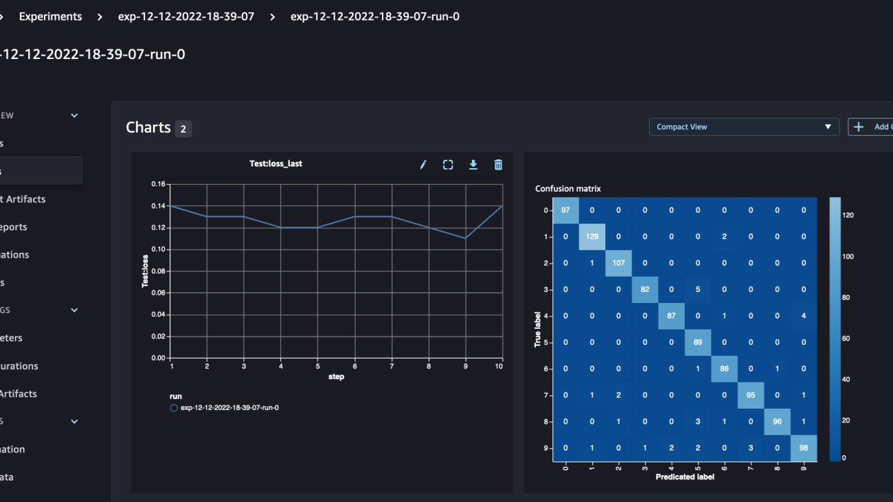
Next generation Amazon SageMaker Experiments – Organize, track, and compare your machine learning trainings at scale
Today, we’re happy to announce updates to our Amazon SageMaker Experiments capability of Amazon SageMaker that lets you organize, track, compare and evaluate machine learning (ML) experiments and model versions from any integrated development environment (IDE) using the SageMaker Python SDK or boto3, including local Jupyter Notebooks.
Machine learning (ML) is an iterative process. When solving a new use case, data scientists and ML engineers iterate through various parameters to find the best model configurations (aka hyperparameters) that can be used in production to solve the identified business challenge. Over time, after experimenting with multiple models and hyperparameters, it becomes difficult for ML teams to efficiently manage model runs to find the optimal one without a tool to keep track of the different experiments. Experiment tracking systems streamline the processes to compare different iterations and helps simplify collaboration and communication in a team, thereby increasing productivity and saving time. This is achieved by organizing and managing ML experiments in an effortless way to draw conclusions from them, for example, finding the training run with the best accuracy.
To solve this challenge, SageMaker provides SageMaker Experiments, a fully integrated SageMaker capability. It provides the flexibility to log your model metrics, parameters, files, artifacts, plot charts from the different metrics, capture various metadata, search through them and support model reproducibility. Data scientists can quickly compare the performance and hyperparameters for model evaluation through visual charts and tables. They can also use SageMaker Experiments to download the created charts and share the model evaluation with their stakeholders.

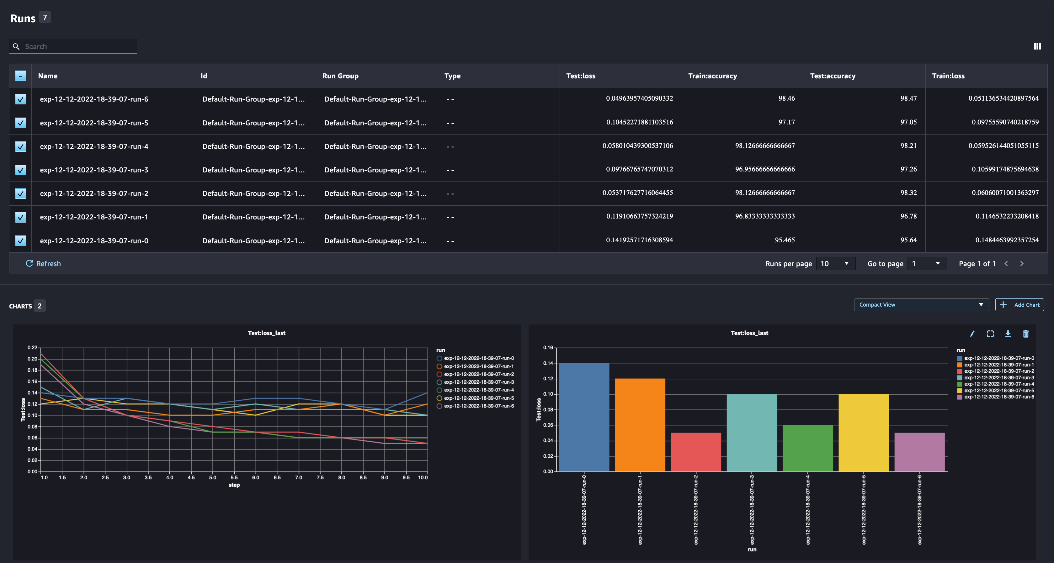
With the new updates to SageMaker Experiments, it is now a part of the SageMaker SDK, simplifying the data scientist work and eliminating the need to install an extra library to manage multiple model executions. We are introducing the following new core concepts:
- Experiment: A collection of runs that are grouped together. An experiment includes runs for multiple types that can be initiated from anywhere using the SageMaker Python SDK.
- Run: Each execution step of a model training process. A run consists of all the inputs, parameters, configurations, and results for one iteration of model training. Custom parameters and metrics can be logged using the
log_parameter,log_parameters, andlog_metricfunctions. Custom input and output can be logged using thelog_filefunction.
The concepts that are implemented as part of a Run class are made available from any IDE where the SageMaker Python SDK is installed. For SageMaker Training, Processing and
Transform Jobs, the SageMaker Experiment Run is automatically passed to the job if the job is invoked within a run context. You can recover the run object using load_run() from your job. Finally, with the new functionalities’ integration, data scientists can also automatically log a confusion matrix, precision and recall graphs, and a ROC curve for classification use cases using the run.log_confusion_matrix, run.log_precision_recall, and run.log_roc_curve functions, respectively.
In this blog post, we will provide examples of how to use the new SageMaker Experiments functionalities in a Jupyter notebook via the SageMaker SDK. We will demonstrate these capabilities using a PyTorch example to train an MNIST handwritten digits classification example. The experiment will be organized as follow:
- Creating experiment’s runs and logging parameters: We will first create a new experiment, start a new run for this experiment, and log parameters to it.
- Logging model performance metrics:We will log model performance metrics and plot metric graphs.
- Comparing model runs:We will compare different model runs according to the model hyperparameters. We will discuss how to compare those runs and how to use SageMaker Experiments to select the best model.
- Running experiments from SageMaker jobs: We will also provide an example of how to automatically share your experiment’s context with a SageMaker processing, training or batch transform job. This allows you to automatically recover your run context with the
load_runfunction inside your job. - Integrating SageMaker Clarify reports: We will demonstrate how we can now integrate SageMaker Clarify bias and explainability reports to a single view with your trained model report.
Prerequisites
For this blog post, we will use Amazon SageMaker Studio to showcase how to log metrics from a Studio notebook using the updated SageMaker Experiments functionalities. To execute the commands presented in our example, you need the following prerequisites:
- SageMaker Studio Domain
- SageMaker Studio user profile with SageMaker full access
- A SageMaker Studio notebook with at least an
ml.t3.mediuminstance type
If you do not have a SageMaker Domain and user profile available, you can create one using this quick setup guide.
Logging parameters
For this exercise, we will use torchvision, a PyTorch package that provides popular datasets, model architectures, and common image transformations for computer vision. SageMaker Studio provides a set of Docker images for common data science use cases that are made available in Amazon ECR. For PyTorch, you have the option of selecting images optimized for CPU or GPU training. For this example, we will select the image PyTorch 1.12 Python 3.8 CPU Optimized and the Python 3 kernel. The examples described below will focus on the SageMaker Experiments functionalities and are not code complete.
Let’s download the data with the torchvision package and track the number of data samples for the train and test datasets as parameters with SageMaker Experiments. For this example, let’s assume train_set and test_set as already downloaded torchvision datasets.
In this example, we use the run.log_parameters to log the number of train and test data samples and run.log_file to upload the raw datasets to Amazon S3 and log them as inputs to our experiment.
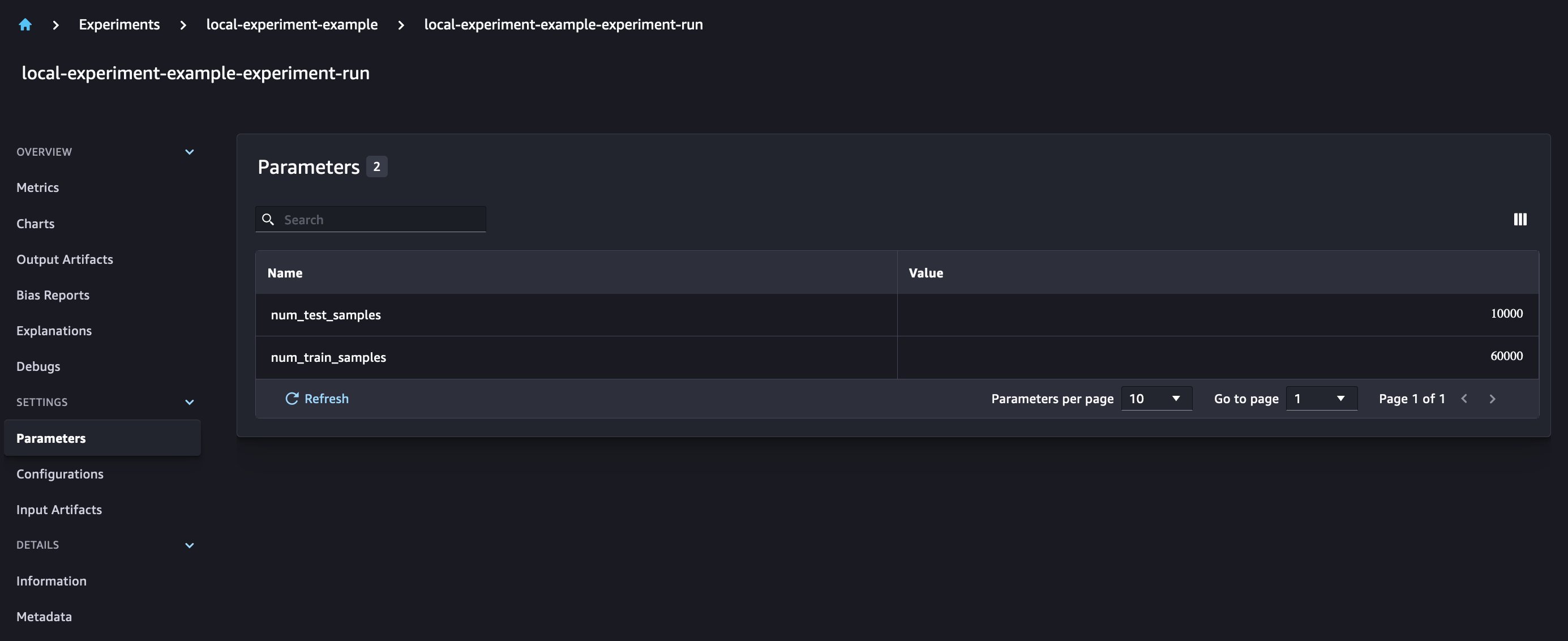

Training a model and logging model metrics
Now that we’ve downloaded our MNIST dataset, let’s train a CNN model to recognize the digits. While training the model, we want to load our existing experiment run, log new parameters to it, and track the model performance by logging model metrics.
We can use the load_run function to load our previous run and use it to log our model training
We can then use run.log_parameter and run.log_parameters to log one or multiple model parameters to our run.
And we can use run.log_metric to log performance metrics to our experiment.
For classification models, you can also use run.log_confusion_matrix, run.log_precision_recall, and run.log_roc_curve, to automatically plot the confusion matrix, precision recall graph, and the ROC curve of your model. Since our model solves a multiclass classification problem, let’s log only the confusion matrix for it.
When looking at our run details, we can now see the generated metrics as shown in the screenshot below:
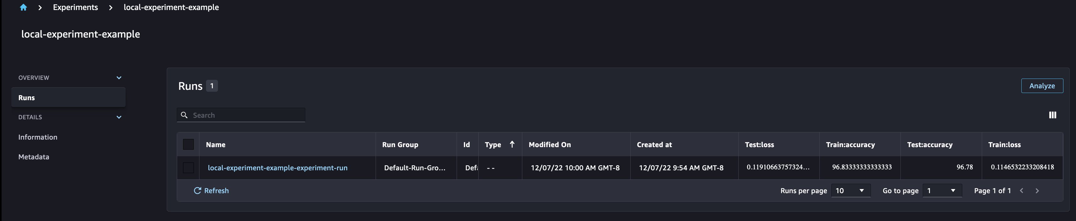
The run details page provides further information about the metrics.

And the new model parameters are tracked on the parameters overview page.

You can also analyze your model performance by class using the automatically plotted confusion matrix, which can also be downloaded and used for different reports. And you can plot extra graphs to analyze the performance of your model based on the logged metrics.
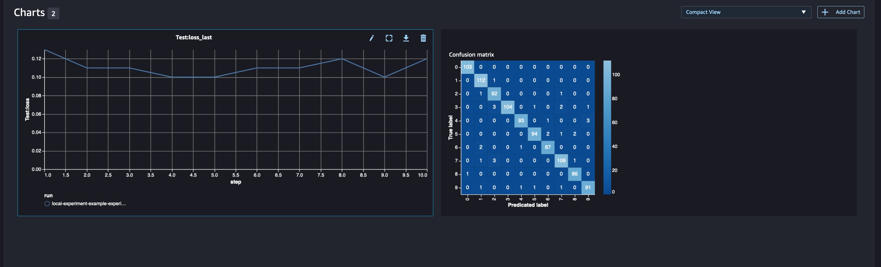
Comparing multiple model parameters
As a data scientist, you want to find the best possible model. That includes training a model multiple times with different hyperparameters and comparing the performance of the model with those hyperparameters. To do so, SageMaker Experiments allows us to create multiple runs in the same experiment. Let’s explore this concept by training our model with different num_hidden_channels and optimizers.
We are now creating six new runs for our experiment. Each one will log the model parameters, metrics, and confusion matrix. We can then compare the runs to select the best-performing model for the problem. When analyzing the runs, we can plot the metric graphs for the different runs as a single plot, comparing the performance of the runs across the different training steps (or epochs).
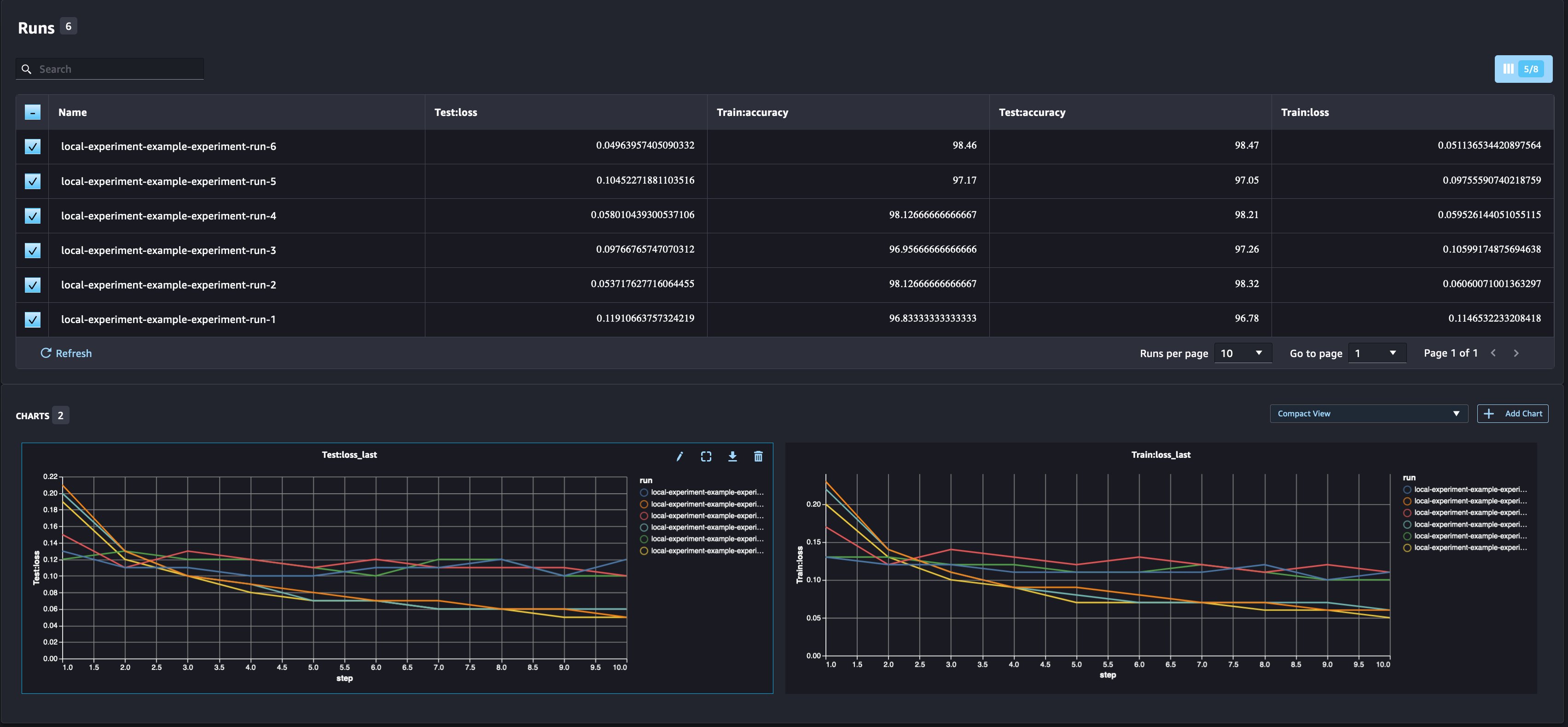
Using SageMaker Experiments with SageMaker training, processing and batch transform jobs
In the example above, we used SageMaker Experiments to log model performance from a SageMaker Studio notebook where the model was trained locally in the notebook. We can do the same to log model performance from SageMaker processing, training and batch transform jobs. With the new automatic context passing capabilities, we do not need to specifically share the experiment configuration with the SageMaker job, as it will be automatically captured.
The example below will focus on the SageMaker Experiments functionalities and is not code complete.
In our model script file, we can get the run context using load_run(). In SageMaker processing and training jobs, we do not need to provide the experiment configuration for loading the configuration. For batch transform jobs, we need to provide experiment_name and run_name to load the experiment’s configuration.
In addition to the information we get when running SageMaker Experiments from a notebook script, the run from a SageMaker job will automatically populate the job parameters and outputs.

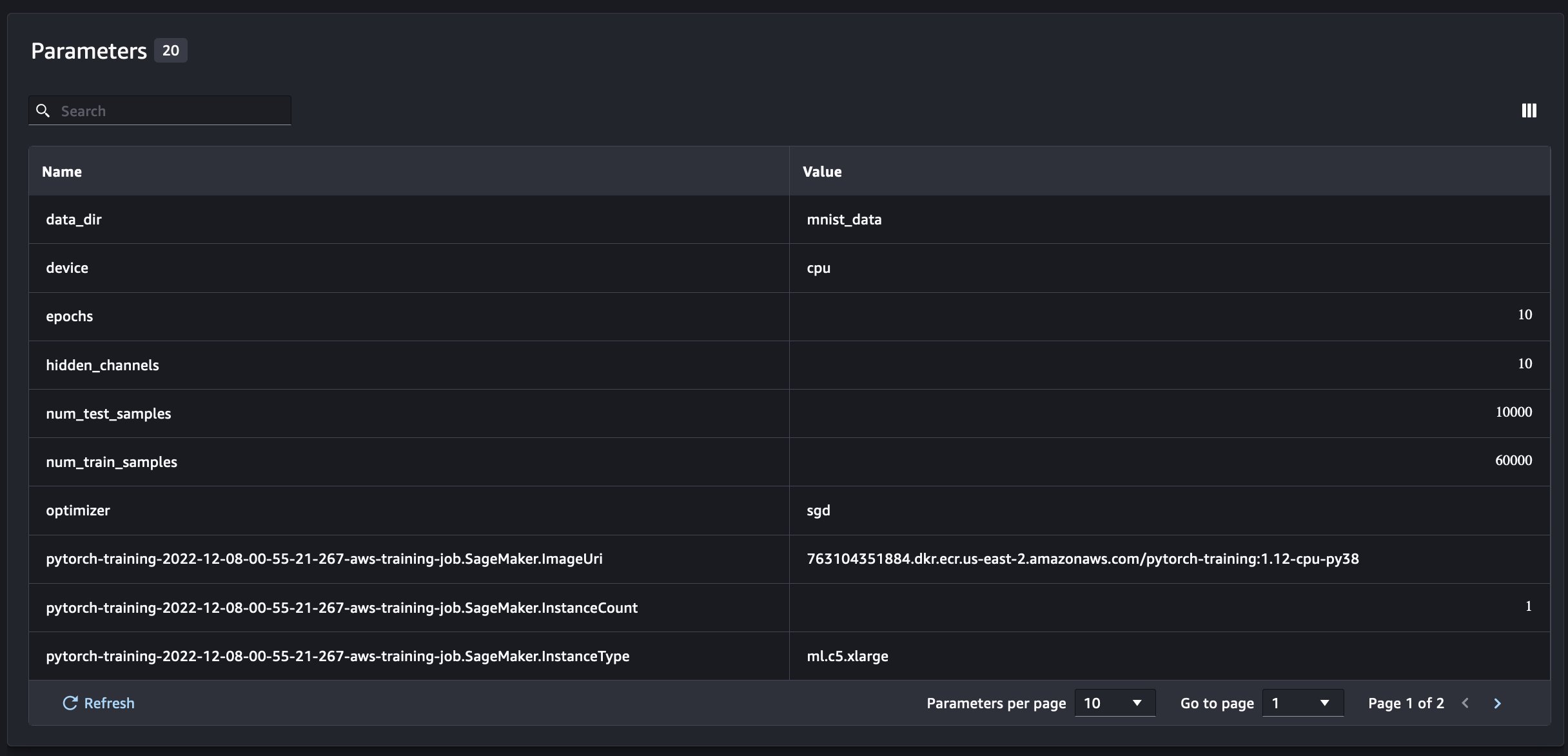
The new SageMaker Experiments SDK also ensures backwards compatibility with the previous version using the concepts of trials and trial components. Any experiment triggered using the previous SageMaker Experiments version will be automatically made available in the new UI, for analyzing the experiments.
Integrating SageMaker Clarify and model training reports
SageMaker Clarify helps improve our ML models by detecting potential bias and helping explain how these models make predictions. Clarify provides pre-built containers that run as SageMaker processing jobs after your model has been trained, using information about your data (data configuration), model (model configuration), and the sensitive data columns that we want to analyze for possible bias (bias configuration). Up until now, SageMaker Experiments displayed our model training and Clarify reports as individual trial components that were connected via a trial.
With the new SageMaker Experiments, we can also integrate SageMaker Clarify reports with our model training having one source of truth that allows us to further understand our model. For an integrated report, all we need to do is to have the same run name for our training and Clarify jobs. The following example demonstrates how we can integrate the reports using an XGBoost model to predict the income of adults across the United States. The model uses the UCI Adult dataset. For this exercise, we assume that the model was already trained and that we already calculated the data, model, and bias configurations.
With this setup, we get a combined view that includes the model metrics, joint inputs and outputs, and the Clarify reports for model statistical bias and explainability.
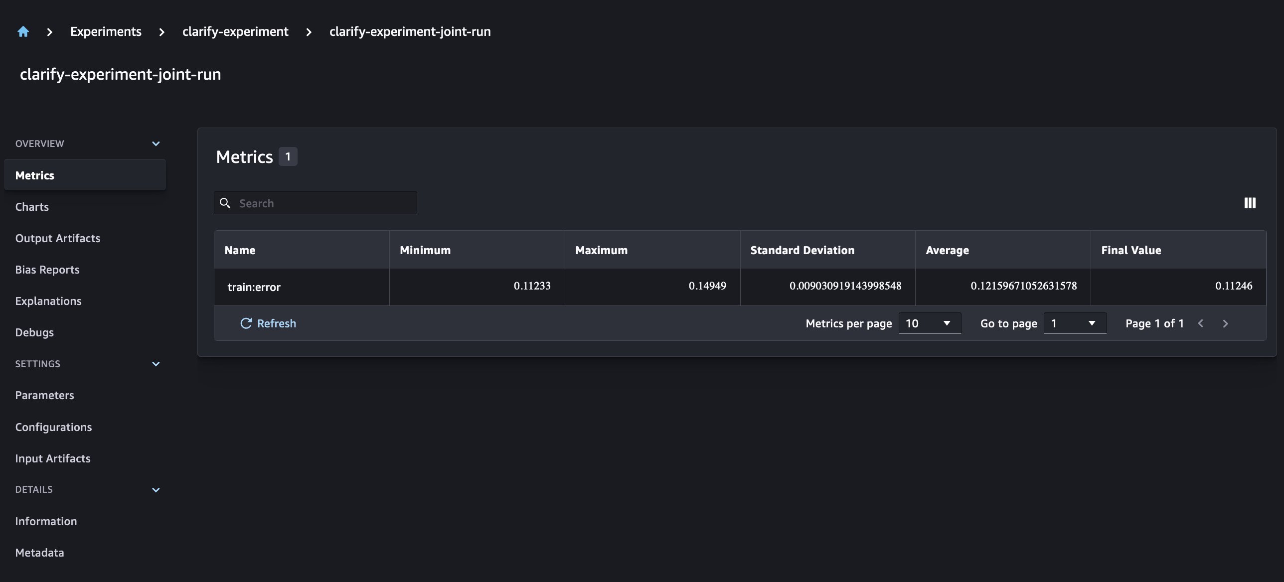


Conclusion
In this post, we explored the new generation of SageMaker Experiments, an integrated part of SageMaker SDK. We demonstrated how to log your ML workflows from anywhere with the new Run class. We presented the new Experiments UI that allows you to track your experiments and plot graphs for a single run metric as well as to compare multiple runs with the new analysis capability. We provided examples of logging experiments from a SageMaker Studio notebook and from a SageMaker Studio training job. Finally, we showed how to integrate model training and SageMaker Clarify reports in a unified view, allowing you to further understand your model.
We encourage you to try out the new Experiments functionalities and connect with the Machine Learning & AI community if you have any questions or feedback!
About the Authors
 Maira Ladeira Tanke is a Machine Learning Specialist at AWS. With a background in Data Science, she has 9 years of experience architecting and building ML applications with customers across industries. As a technical lead, she helps customers accelerate their achievement of business value through emerging technologies and innovative solutions. In her free time, Maira enjoys traveling and spending time with her family someplace warm.
 Mani Khanuja is an Artificial Intelligence and Machine Learning Specialist SA at Amazon Web Services (AWS). She helps customers using machine learning to solve their business challenges using the AWS. She spends most of her time diving deep and teaching customers on AI/ML projects related to computer vision, natural language processing, forecasting, ML at the edge, and more. She is passionate about ML at edge, therefore, she has created her own lab with self-driving kit and prototype manufacturing production line, where she spends lot of her free time.
 Dewen Qi is a Software Development Engineer at AWS. She currently participating in building a collection of platform services and tools in AWS SageMaker to help customer in making their ML projects successful. She is also passionate about bringing the concept of MLOps to broader audience. Outside of work, Dewen enjoys practicing Cello.
 Abhishek Agarwal is a Senior Product Manager for Amazon SageMaker. He is passionate about working with customers and making machine learning more accessible. In his spare time, Abhishek enjoys painting, biking and learning about innovative technologies.
 Dana Benson is a Software Engineer working in the Amazon SageMaker Experiments, Lineage, and Search team. Prior to joining AWS, Dana spent time enabling smart home functionality in Alexa and mobile ordering at Starbucks.
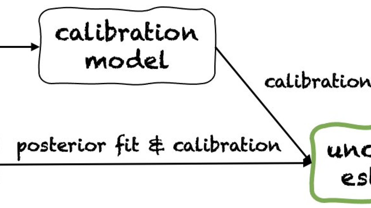
Introducing Fortuna: A library for uncertainty quantification
Proper estimation of predictive uncertainty is fundamental in applications that involve critical decisions. Uncertainty can be used to assess the reliability of model predictions, trigger human intervention, or decide whether a model can be safely deployed in the wild.
We introduce Fortuna, an open-source library for uncertainty quantification. Fortuna provides calibration methods, such as conformal prediction, that can be applied to any trained neural network to obtain calibrated uncertainty estimates. The library further supports a number of Bayesian inference methods that can be applied to deep neural networks written in Flax. The library makes it easy to run benchmarks and will enable practitioners to build robust and reliable AI solutions by taking advantage of advanced uncertainty quantification techniques.
The problem of overconfidence in deep learning
If you have ever looked at class probabilities returned by a trained deep neural network classifier, you might have observed that the probability of one class was much larger than the others. Something like this, for example:
p = [0.0001, 0.0002, …, 0.9991, 0.0003, …, 0.0001]
If this is the case for the majority of the predictions, your model might be overconfident. In order to evaluate the validity of the probabilities returned by the classifier, we may compare them with the actual accuracy achieved over a holdout data set. Indeed, it is natural to assume that the proportion of correctly classified data points should approximately match the estimated probability of the predicted class. This concept is known as calibration [Guo C. et al., 2017].
Unfortunately, many trained deep neural networks are miscalibrated, meaning that the estimated probability of the predicted class is much higher than the proportion of correctly classified input data points. In other words, the classifier is overconfident.
Being overconfident might be problematic in practice. A doctor may not order relevant additional tests, as a result of an overconfident healthy diagnosis produced by an AI. A self-driving car may decide not to brake because it confidently assessed that the object in front was not a person. A governor may decide to evacuate a town because the probability of an eminent natural disaster estimated by an AI is too high. In these and many other applications, calibrated uncertainty estimates are critical to assess the reliability of model predictions, fall back to a human decision-maker, or decide whether a model can be safely deployed.
Fortuna: A library for uncertainty quantification
There are many published techniques to either estimate or calibrate the uncertainty of predictions, e.g., Bayesian inference [Wilson A.G., 2020], temperature scaling [Guo C. et al., 2017], and conformal prediction [Angelopoulos A.N. et al., 2022] methods. However, existing tools and libraries for uncertainty quantification have a narrow scope and do not offer a breadth of techniques in a single place. This results in a significant overhead, hindering the adoption of uncertainty into production systems.
In order to fill this gap, we launch Fortuna, a library for uncertainty quantification that brings together prominent methods across the literature and makes them available to users with a standardized and intuitive interface.
As an example, suppose you have training, calibration, and test data loaders in tensorflow.Tensor format, namely train_data_loader, calib_data_loader and test_data_loader. Furthermore, you have a deep learning model written in Flax, namely model. Then you can use Fortuna to:
- fit a posterior distribution;
- calibrate the model outputs;
- make calibrated predictions;
- estimate uncertainty estimates;
- compute evaluation metrics.
The following code does all of this for you.
The code above makes use of several default choices, including SWAG [Maddox W.J. et al., 2019] as a posterior inference method, temperature scaling [Guo C. et al., 2017] to calibrate the model outputs, and a standard Gaussian prior distribution, as well as the configuration of the posterior fitting and calibration processes. You can easily configure all of these components, and you are highly encouraged to do so if you are looking for a specific configuration or if you want to compare several ones.
Usage modes
Fortuna offers three usage modes: 1/ Starting from Flax models, 2/ Starting from model outputs, and 3/ Starting from uncertainty estimates. Their pipelines are depicted in the following figure, each starting from one of the green panels. The code snippet above is an example of using Fortuna starting from Flax models, which allows training a model using Bayesian inference procedures. Alternatively, you can start either by model outputs or directly from your own uncertainty estimates. Both these latter modes are framework independent and help you obtain calibrated uncertainty estimates starting from a trained model.
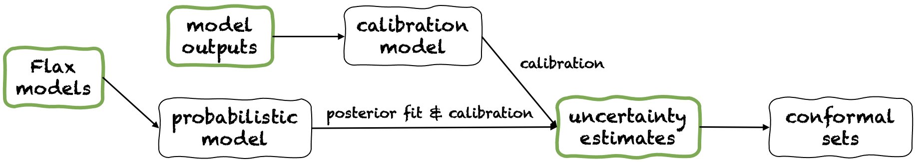
1/ Starting from uncertainty estimates
Starting from uncertainty estimates has minimal compatibility requirements, and it is the quickest level of interaction with the library. This usage mode offers conformal prediction methods for both classification and regression. These take uncertainty estimates in numpy.ndarray format and return rigorous sets of predictions that retain a user-given level of probability. In one-dimensional regression tasks, conformal sets may be thought of as calibrated versions of confidence or credible intervals.
Mind that if the uncertainty estimates that you provide in inputs are inaccurate, conformal sets might be large and unusable. For this reason, if your application allows it, please consider the Starting from model outputs and Starting from Flax models usage modes detailed below.
2/ Starting from model outputs
This mode assumes you have already trained a model in some framework and arrive at Fortuna with model outputs in numpy.ndarray format for each input data point. This usage mode allows you to calibrate your model outputs, estimate uncertainty, compute metrics, and obtain conformal sets.
Compared to the Starting from uncertainty estimates usage mode, Starting from model outputs provides better control, as it can make sure uncertainty estimates have been appropriately calibrated. However, if the model had been trained with classical methods, the resulting quantification of model (aka epistemic) uncertainty may be poor. To mitigate this problem, please consider the Starting from Flax models usage mode.
3/ Starting from Flax models
Starting from Flax models has higher compatibility requirements than the Starting from uncertainty estimates and Starting from model outputs usage modes, as it requires deep learning models written in Flax. However, it enables you to replace standard model training with scalable Bayesian inference procedures, which may significantly improve the quantification of predictive uncertainty.
Bayesian methods work by representing uncertainty over which solution is correct, given limited information, through uncertainty over model parameters. This type of uncertainty is called “epistemic” uncertainty. Because neural networks can represent many different solutions, corresponding to different settings of their parameters, Bayesian methods can be especially impactful in deep learning. We provide many scalable Bayesian inference procedures, which can often be used to provide uncertainty estimates, as well as improved accuracy and calibration, with essentially no training-time overhead.
Conclusion
We announced the general availability of Fortuna, a library for uncertainty quantification in deep learning. Fortuna brings together prominent methods across the literature, e.g., conformal methods, temperature scaling, and Bayesian inference, and makes them available to users with a standardized and intuitive interface. To get started with Fortuna, you can consult the following resources:
Try Fortuna out, and let us know what you think! You are encouraged to contribute to the library or leave your suggestions and contributions—just create an issue or open a pull request. On our side, we will keep on improving Fortuna, increase its coverage of uncertainty quantification methods and add further examples that showcase its usefulness in several scenarios.
About the authors

Gianluca Detommaso is an Applied Scientist at AWS. He currently works on uncertainty quantification in deep learning. In his spare time, Gianluca likes to practice sports, eating great food and learning new skills.
 Alberto Gasparin is an Applied Scientist within Amazon Community Shopping since July 2021. His interests include natural language processing, information retrieval and uncertainty quantification. He is a food and wine enthusiast.
 Michele Donini is a Sr Applied Scientist at AWS. He leads a team of scientists working on Responsible AI and his research interests are Algorithmic Fairness and Explainable Machine Learning.
 Matthias Seeger is a Principal Applied Scientist at AWS.
Cedric Archambeau is a Principal Applied Scientist at AWS and Fellow of the European Lab for Learning and Intelligent Systems.
 Andrew Gordon Wilson is an Associate Professor at the Courant Institute of Mathematical Sciences and Center for Data Science at New York University, and an Amazon Visiting Academic at AWS. He is particularly engaged in building methods for Bayesian and probabilistic deep learning, scalable Gaussian processes, Bayesian optimization, and physics-inspired machine learning.