This is a guest post co-written by Julian Blau, Data Scientist at xarvio Digital Farming Solutions; BASF Digital Farming GmbH, and Antonio Rodriguez, AI/ML Specialist Solutions Architect at AWS
xarvio Digital Farming Solutions is a brand from BASF Digital Farming GmbH, which is part of BASF Agricultural Solutions division. xarvio Digital Farming Solutions offers precision digital farming products to help farmers optimize crop production. Available globally, xarvio products use machine learning (ML), image recognition technology, and advanced crop and disease models, in combination with data from satellites and weather station devices, to deliver accurate and timely agronomic recommendations to manage the needs of individual fields. xarvio products are tailored to local farming conditions, can monitor growth stages, and recognize diseases and pests. They increase efficiency, save time, reduce risks, and provide higher reliability for planning and decision-making—all while contributing to sustainable agriculture.
We work with different geospatial data, including satellite imagery of the areas where our users’ fields are located, for some of our use cases. Therefore, we use and process hundreds of large image files daily. Initially, we had to invest a lot of manual work and effort to ingest, process, and analyze this data using third-party tools, open-source libraries, or general-purpose cloud services. In some instances, this could take up to 2 months for us to build the pipelines for each specific project. Now, by utilizing the geospatial capabilities of Amazon SageMaker, we have reduced this time to just 1–2 weeks.
This time-saving is the result of automating the geospatial data pipelines to deliver our use cases more efficiently, along with using built-in reusable components for speeding up and improving similar projects in other geographical areas, while applying the same proven steps for other use cases based on similar data.
In this post, we go through an example use case to describe some of the techniques we commonly use, and show how implementing these using SageMaker geospatial functionalities in combination with other SageMaker features delivers measurable benefits. We also include code examples so you can adapt these to your own specific use cases.
Overview of solution
A typical remote sensing project for developing new solutions requires a step-by-step analysis of imagery taken by optical satellites such as Sentinel or Landsat, in combination with other data, including weather forecasts or specific field properties. The satellite images provide us with valuable information used in our digital farming solutions to help our users accomplish various tasks:
- Detecting diseases early in their fields
- Planning the right nutrition and treatments to be applied
- Getting insights on weather and water for planning irrigation
- Predicting crop yield
- Performing other crop management tasks
To achieve these goals, our analyses typically require preprocessing of the satellite images with different techniques that are common in the geospatial domain.
To demonstrate the capabilities of SageMaker geospatial, we experimented with identifying agricultural fields through ML segmentation models. Additionally, we explored the preexisting SageMaker geospatial models and the bring your own model (BYOM) functionality on geospatial tasks such as land use and land cover classification, or crop classification, often requiring panoptic or semantic segmentation techniques as additional steps in the process.
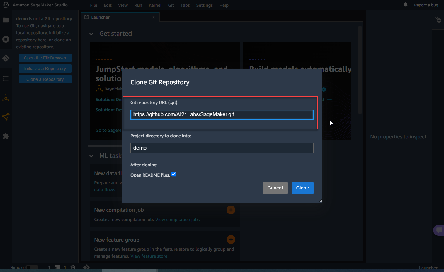
In the following sections, we go through some examples of how to perform these steps with SageMaker geospatial capabilities. You can also follow these in the end-to-end example notebook available in the following GitHub repository.
As previously mentioned, we selected the land cover classification use case, which consists of identifying the type of physical coverage that we have on a given geographical area on the earth’s surface, organized on a set of classes including vegetation, water, or snow. This high-resolution classification allows us to detect the details for the location of the fields and its surroundings with high accuracy, which can be later chained with other analyses such as change detection in crop classification.
Client setup
First, let’s assume we have users with crops being cultivated in a given geographical area that we can identify within a polygon of geospatial coordinates. For this post, we define an example area over Germany. We can also define a given time range, for example in the first months of 2022. See the following code:
### Coordinates for the polygon of your area of interest...
coordinates = [
    [9.181602157004177, 53.14038825707946],
    [9.181602157004177, 52.30629767547948],
    [10.587520893823973, 52.30629767547948],
    [10.587520893823973, 53.14038825707946],
    [9.181602157004177, 53.14038825707946],
]
### Time-range of interest...
time_start = "2022-01-01T12:00:00Z"
time_end = "2022-05-01T12:00:00Z"
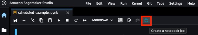
In our example, we work with the SageMaker geospatial SDK through programmatic or code interaction, because we’re interested in building code pipelines that can be automated with the different steps required in our process. Note you could also work with an UI through the graphical extensions provided with SageMaker geospatial in Amazon SageMaker Studio if you prefer this approach, as shown in the following screenshots. For accessing the Geospatial Studio UI, open the SageMaker Studio Launcher and choose Manage Geospatial resources. You can check more details in the documentation to Get Started with Amazon SageMaker Geospatial Capabilities.


Here you can graphically create, monitor, and visualize the results of the Earth Observation jobs (EOJs) that you run with SageMaker geospatial features.
Back to our example, the first step for interacting with the SageMaker geospatial SDK is to set up the client. We can do this by establishing a session with the botocore library:
session = botocore.session.get_session()
gsClient = session.create_client(
    service_name='sagemaker-geospatial',
    region_name=region) #Replace with your region, e.g., 'us-east-1'
From this point on, we can use the client for running any EOJs of interest.
Obtaining data
For this use case, we start by collecting satellite imagery for our given geographical area. Depending on the location of interest, there might be more or less frequent coverage by the available satellites, which have its imagery organized in what is usually referred to as raster collections.
With the geospatial capabilities of SageMaker, you have direct access to high-quality data sources for obtaining the geospatial data directly, including those from AWS Data Exchange and the Registry of Open Data on AWS, among others. We can run the following command to list the raster collections already provided by SageMaker:
list_raster_data_collections_resp = gsClient.list_raster_data_collections()
This returns the details for the different raster collections available, including the Landsat C2L2 Surface Reflectance (SR), Landsat C2L2 Surface Temperature (ST), or the Sentinel 2A & 2B. Conveniently, Level 2A imagery is already optimized into Cloud-Optimized GeoTIFFs (COGs). See the following code:
…
{'Name': 'Sentinel 2 L2A COGs',
  'Arn': 'arn:aws:sagemaker-geospatial:us-west-2:378778860802:raster-data-collection/public/nmqj48dcu3g7ayw8',
  'Type': 'PUBLIC',
  'Description': 'Sentinel-2a and Sentinel-2b imagery, processed to Level 2A (Surface Reflectance) and converted to Cloud-Optimized GeoTIFFs'
…
Let’s take this last one for our example, by setting our data_collection_arn parameter to the Sentinel 2 L2A COGs’ collection ARN.
We can also search the available imagery for a given geographical location by passing the coordinates of a polygon we defined as our area of interest (AOI). This allows you to visualize the image tiles available that cover the polygon you submit for the specified AOI, including the Amazon Simple Storage Service (Amazon S3) URIs for these images. Note that satellite imagery is typically provided in different bands according to the wavelength of the observation; we discuss this more later in the post.
response = gsClient.search_raster_data_collection(**eoj_input_config, Arn=data_collection_arn)
The preceding code returns the S3 URIs for the different image tiles available, that you can directly visualize with any library compatible with GeoTIFFs such as rasterio. For example, let’s visualize two of the True Color Image (TCI) tiles.
…
'visual': {'Href': 'https://sentinel-cogs.s3.us-west-2.amazonaws.com/sentinel-s2-l2a-cogs/32/U/NC/2022/3/S2A_32UNC_20220325_0_L2A/TCI.tif'},
…


Processing techniques
Some of the most common preprocessing techniques that we apply include cloud removal, geo mosaic, temporal statistics, band math, or stacking. All of these processes can now be done directly through the use of EOJs in SageMaker, without the need to perform manual coding or using complex and expensive third-party tools. This makes it 50% faster to build our data processing pipelines. With SageMaker geospatial capabilities, we can run these processes over different input types. For example:
- Directly run a query for any of the raster collections included with the service through the
RasterDataCollectionQuery parameter
- Pass imagery stored in Amazon S3 as an input through the
DataSourceConfig parameter
- Simply chain the results of a previous EOJ through the
PreviousEarthObservationJobArn parameter
This flexibility allows you to build any kind of processing pipeline you need.
The following diagram illustrates the processes we cover in our example.

In our example, we use a raster data collection query as input, for which we pass the coordinates of our AOI and time range of interest. We also specify a percentage of maximum cloud coverage of 2%, because we want clear and noise-free observations of our geographical area. See the following code:
eoj_input_config = {
    "RasterDataCollectionQuery": {
        "RasterDataCollectionArn": data_collection_arn,
        "AreaOfInterest": {
            "AreaOfInterestGeometry": {"PolygonGeometry": {"Coordinates": [coordinates]}}
        },
        "TimeRangeFilter": {"StartTime": time_start, "EndTime": time_end},
        "PropertyFilters": {
            "Properties": [
                {"Property": {"EoCloudCover": {"LowerBound": 0, "UpperBound": 2}}}
            ]
        },
    }
}
For more information on supported query syntax, refer to Create an Earth Observation Job.
Cloud gap removal
Satellite observations are often less useful due to high cloud coverage. Cloud gap filling or cloud removal is the process of replacing the cloudy pixels from the images, which can be done with different methods to prepare the data for further processing steps.
With SageMaker geospatial capabilities, we can achieve this by specifying a CloudRemovalConfig parameter in the configuration of our job.
eoj_config =  {
    'CloudRemovalConfig': {
        'AlgorithmName': 'INTERPOLATION',
        'InterpolationValue': '-9999'
    }
}
Note that we’re using an interpolation algorithm with a fixed value in our example, but there are other configurations supported, as explained in the Create an Earth Observation Job documentation. The interpolation allows it estimating a value for replacing the cloudy pixels, by considering the surrounding pixels.
We can now run our EOJ with our input and job configurations:
response = gsClient.start_earth_observation_job(
    Name =  'cloudremovaljob',
    ExecutionRoleArn = role,
    InputConfig = eoj_input_config,
    JobConfig = eoj_config,
)
This job takes a few minutes to complete depending on the input area and processing parameters.
When it’s complete, the results of the EOJ are stored in a service-owned location, from where we can either export the results to Amazon S3, or chain these as input for another EOJ. In our example, we export the results to Amazon S3 by running the following code:
response = gsClient.export_earth_observation_job(
    Arn = cr_eoj_arn,
    ExecutionRoleArn = role,
    OutputConfig = {
        'S3Data': {
            'S3Uri': f's3://{bucket}/{prefix}/cloud_removal/',
            'KmsKeyId': ''
        }
    }
)
Now we’re able to visualize the resulting imagery stored in our specified Amazon S3 location for the individual spectral bands. For example, let’s inspect two of the blue band images returned.

Alternatively, you can also check the results of the EOJ graphically by using the geospatial extensions available in Studio, as shown in the following screenshots.


Temporal statistics
Because the satellites continuously orbit around earth, the images for a given geographical area of interest are taken at specific time frames with a specific temporal frequency, such as daily, every 5 days, or 2 weeks, depending on the satellite. The temporal statistics process enables us to combine different observations taken at different times to produce an aggregated view, such as a yearly mean, or the mean of all observations in a specific time range, for the given area.
With SageMaker geospatial capabilities, we can do this by setting the TemporalStatisticsConfig parameter. In our example, we obtain the yearly mean aggregation for the Near Infrared (NIR) band, because this band can reveal vegetation density differences below the top of the canopies:
eoj_config =  {
    'TemporalStatisticsConfig': {
        'GroupBy': 'YEARLY',
        'Statistics': ['MEAN'],
        'TargetBands': ['nir']
    }
}
After a few minutes running an EOJ with this config, we can export the results to Amazon S3 to obtain imagery like the following examples, in which we can observe the different vegetation densities represented with different color intensities. Note the EOJ can produce multiple images as tiles, depending on the satellite data available for the time range and coordinates specified.


Band math
Earth observation satellites are designed to detect light in different wavelengths, some of which are invisible to the human eye. Each range contains specific bands of the light spectrum at different wavelengths, which combined with arithmetic can produce images with rich information about characteristics of the field such as vegetation health, temperature, or presence of clouds, among many others. This is performed in a process commonly called band math or band arithmetic.
With SageMaker geospatial capabilities, we can run this by setting the BandMathConfig parameter. For example, let’s obtain the moisture index images by running the following code:
eoj_config =  {
    'BandMathConfig': {
        'CustomIndices': {
            'Operations': [
                {
                    'Name': 'moisture',
                    'Equation': '(B8A - B11) / (B8A + B11)'
                }
            ]
        }
    }
}
After a few minutes running an EOJ with this config, we can export the results and obtain images, such as the following two examples.


Stacking
Similar to band math, the process of combining bands together to produce composite images from the original bands is called stacking. For example, we could stack the red, blue, and green light bands of a satellite image to produce the true color image of the AOI.
With SageMaker geospatial capabilities, we can do this by setting the StackConfig parameter. Let’s stack the RGB bands as per the previous example with the following command:
eoj_config =  {
    'StackConfig': {
        'OutputResolution': {
            'Predefined': 'HIGHEST'
        },
        'TargetBands': ['red', 'green', 'blue']
    }
}
After a few minutes running an EOJ with this config, we can export the results and obtain images.


Semantic segmentation models
As part of our work, we commonly use ML models to run inferences over the preprocessed imagery, such as detecting cloudy areas or classifying the type of land in each area of the images.
With SageMaker geospatial capabilities, you can do this by relying on the built-in segmentation models.
For our example, let’s use the land cover segmentation model by specifying the LandCoverSegmentationConfig parameter. This runs inferences on the input by using the built-in model, without the need to train or host any infrastructure in SageMaker:
response = gsClient.start_earth_observation_job(
    Name =  'landcovermodeljob',
    ExecutionRoleArn = role,
    InputConfig = eoj_input_config,
    JobConfig = {
        'LandCoverSegmentationConfig': {},
    },
)
After a few minutes running a job with this config, we can export the results and obtain images.


In the preceding examples, each pixel in the images corresponds to a land type class, as shown in the following legend.

This allows us to directly identify the specific types of areas in the scene such as vegetation or water, providing valuable insights for additional analyses.
Bring your own model with SageMaker
If the state-of-the-art geospatial models provided with SageMaker aren’t enough for our use case, we can also chain the results of any of the preprocessing steps shown so far with any custom model onboarded to SageMaker for inference, as explained in this SageMaker Script Mode example. We can do this with any of the inference modes supported in SageMaker, including synchronous with real-time SageMaker endpoints, asynchronous with SageMaker asynchronous endpoints, batch or offline with SageMaker batch transforms, and serverless with SageMaker serverless inference. You can check further details about these modes in the Deploy Models for Inference documentation. The following diagram illustrates the workflow in high-level.

For our example, let’s assume we have onboarded two models for performing a land cover classification and crop type classification.
We just have to point towards our trained model artifact, in our example a PyTorch model, similar to the following code:
from sagemaker.pytorch import PyTorchModel
import datetime

model = PyTorchModel(
    name=model_name, ### Set a model name
    model_data=MODEL_S3_PATH, ### Location of the custom model in S3
    role=role,
    entry_point='inference.py', ### Your inference entry-point script
    source_dir='code', ### Folder with any dependencies
    image_uri=image_uri, ### URI for your AWS DLC or custom container
    env={
        'TS_MAX_REQUEST_SIZE': '100000000',
        'TS_MAX_RESPONSE_SIZE': '100000000',
        'TS_DEFAULT_RESPONSE_TIMEOUT': '1000',
    }, ### Optional – Set environment variables for max size and timeout
)

predictor = model.deploy(
    initial_instance_count = 1, ### Your number of instances
    instance_type = 'ml.g4dn.8xlarge', ### Your instance type
    async_inference_config=sagemaker.async_inference.AsyncInferenceConfig(
        output_path=f"s3://{bucket}/{prefix}/output",
        max_concurrent_invocations_per_instance=2,
    ), ### Optional – Async config if using SageMaker Async Endpoints
)

predictor.predict(data) ### Your images for inference
This allows you to obtain the resulting images after inference, depending on the model you’re using.
In our example, when running a custom land cover segmentation, the model produces images similar to the following, where we compare the input and prediction images with its corresponding legend.

 .
. 
The following is another example of a crop classification model, where we show the comparison of the original vs. resulting panoptic and semantic segmentation results, with its corresponding legend.

Automating geospatial pipelines
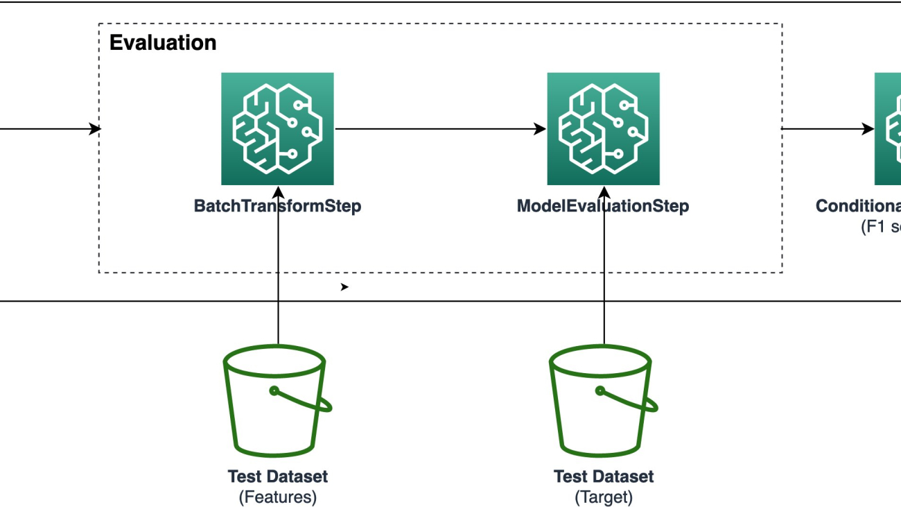
Finally, we can also automate the previous steps by building geospatial data processing and inference pipelines with Amazon SageMaker Pipelines. We simply chain each preprocessing step required through the use of Lambda Steps and Callback Steps in Pipelines. For example, you could also add a final inference step using a Transform Step, or directly through another combination of Lambda Steps and Callback Steps, for running an EOJ with one of the built-in semantic segmentation models in SageMaker geospatial features.
Note we’re using Lambda Steps and Callback Steps in Pipelines because the EOJs are asynchronous, so this type of step allows us to monitor the run of the processing job and resume the pipeline when it’s complete through messages in an Amazon Simple Queue Service (Amazon SQS) queue.

You can check the notebook in the GitHub repository for a detailed example of this code.
Now we can visualize the diagram of our geospatial pipeline through Studio and monitor the runs in Pipelines, as shown in the following screenshot.

Conclusion
In this post, we presented a summary of the processes we implemented with SageMaker geospatial capabilities for building geospatial data pipelines for our advanced products from xarvio Digital Farming Solutions. Using SageMaker geospatial increased the efficiency of our geospatial work by more than 50%, through the use of pre-built APIs that accelerate and simplify our preprocessing and modeling steps for ML.
As a next step, we’re onboarding more models from our catalog to SageMaker to continue the automation of our solution pipelines, and will continue utilizing more geospatial features of SageMaker as the service evolves.
We encourage you to try SageMaker geospatial capabilities by adapting the end-to-end example notebook provided in this post, and learning more about the service in What is Amazon SageMaker Geospatial Capabilities?.
About the Authors
 Julian Blau is a Data Scientist at BASF Digital Farming GmbH, located in Cologne, Germany. He develops digital solutions for agriculture, addressing the needs of BASF’s global customer base by using geospatial data and machine learning. Outside work, he enjoys traveling and being outdoors with friends and family.
 Antonio Rodriguez is an Artificial Intelligence and Machine Learning Specialist Solutions Architect in Amazon Web Services, based out of Spain. He helps companies of all sizes solve their challenges through innovation, and creates new business opportunities with AWS Cloud and AI/ML services. Apart from work, he loves to spend time with his family and play sports with his friends.
Read More


 Sean Morgan is a Senior ML Solutions Architect at AWS. He has experience in the semiconductor and academic research fields, and uses his experience to help customers reach their goals on AWS. In his free time Sean is an activate open source contributor/maintainer and is the special interest group lead for TensorFlow Addons.
 Sumedha Swamy is a Principal Product Manager at Amazon Web Services. He leads SageMaker Studio team to build it into the IDE of choice for interactive data science and data engineering workflows. He has spent the past 15 years building customer-obsessed consumer and enterprise products using Machine Learning. In his free time he likes photographing the amazing geology of the American Southwest.
 Edward Sun is a Senior SDE working for SageMaker Studio at Amazon Web Services. He is focused on building interactive ML solution and simplifying the customer experience to integrate SageMaker Studio with popular technologies in data engineering and ML ecosystem. In his spare time, Edward is big fan of camping, hiking and fishing and enjoys the time spending with his family.
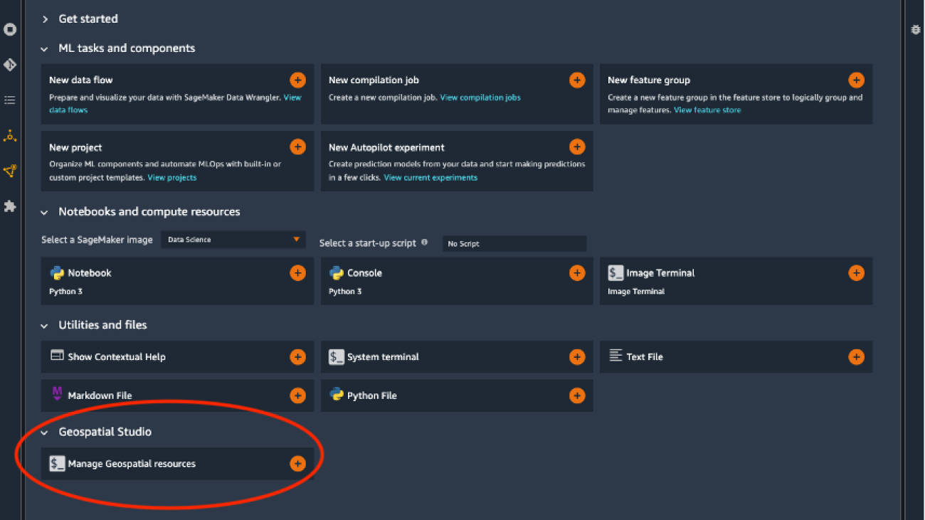


 Vasi Philomin is currently a Vice President in the AWS AI team for services in the language and speech technologies areas such as Amazon Lex, Amazon Polly, Amazon Translate, Amazon Transcribe/Transcribe Medical, Amazon Comprehend, Amazon Kendra, Amazon Code Whisperer, Amazon Monitron, Amazon Lookout for Equipment and Contact Lens/Voice ID for Amazon Connect as well as Machine Learning Solutions Lab and Responsible AI.