Posts in category: Amazon AWS

Today, we’re excited to announce that Amazon SageMaker now supports the ability to configure Instance Metadata Service Version 2 (IMDSv2) for Notebook Instances, and for administrators to control the minimum version with which end-users create new Notebook Instances. You can now choose IMDSv2 only for your new and existing SageMaker Notebook Instances to take advantage of the latest protection and support provided by IMDSv2.

Instance metadata is data about your instance that you can use to configure or manage the running instance, by providing temporary and frequently rotated credentials that can only be accessed by software running on the instance. IMDS makes metadata about the instance, such as its network and storage, available through a special link-local IP address of 169.254.169.254. You can use IMDS on your SageMaker Notebook Instances, similar to how you would use IMDS on an Amazon Elastic Compute Cloud (Amazon EC2) instance. For detailed documentation, see Instance metadata and user data.

The release of IMDSv2 adds an additional layer of protection using session authentication. With IMDSv2, each session starts with a PUT request to IMDSv2 to get a secure token, with an expiry time, which can be a minimum of 1 second and a maximum of 6 hours. Any subsequent GET request to IMDS must send the resulting token as a header, in order to receive a successful response. When the specified duration expires, a new token is required for future requests.

A sample IMDSv1 call looks like the following code:

curl http://169.254.169.254/latest/meta-data/profile

With IMDSv2, the call looks like the following code:

TOKEN=`curl -X PUT "http://169.254.169.254/latest/api/token" -H "X-aws-ec2-metadata-token-ttl-seconds: 21600"` 

curl http://169.254.169.254/latest/meta-data/profile -H "X-aws-ec2-metadata-token: $TOKEN"

Adopting IMDSv2 and setting it as the minimum version offers various security benefits over IMDSv1. IMDSv2 protects against unrestricted Web Application Firewall (WAF) configurations, open reverse proxies, Server-Side Request Forgery (SSRF) vulnerabilities, and open layer 3 firewalls and NATs that could be used to access the instance metadata. For a detailed comparison, see Add defense in depth against open firewalls, reverse proxies, and SSRF vulnerabilities with enhancements to the EC2 Instance Metadata Service.

In this post, we show you how to configure your SageMaker notebooks with IMDSv2 only support. We also share the support plan for IMDSv1, and how you can enforce IMDSv2 on your notebooks.

What’s new with IMDSv2 support and SageMaker

You can now configure the IMDS version of SageMaker Notebook Instances while creating or updating the instance, which you can do via the SageMaker API or the SageMaker Console, with the minimum IMDS version parameter. The minimum IMDS version specifies the minimum supported version. Setting to a value of 1 allows support for both IMDSv1 and IMDSv2, and setting the minimum version to 2 supports only IMDSv2. With an IMDSv2-only notebook, you can leverage the additional defense in depth that IMDSv2 provides.

We also provide a SageMaker condition key for IAM policies that allows you to restrict the IMDS version for Notebook Instances through the CreateNotebookInstance and UpdateNotebookInstance API calls. Administrators can use this condition key to restrict their end users to creating and/or updating notebooks to support IMDSv2 only. You can add this condition key to the AWS Identity and Access Management (IAM) policy attached to IAM users, roles or groups responsible for creating and updating notebooks.

Additionally, you can also switch between IMDS version configurations using the minimum IMDS version parameter in the SageMaker UpdateNotebookInstance API.

Support for configuring the IMDS version and restricting the IMDS version to v2 only is now available in all AWS Regions in which SageMaker Notebook Instances are available.

Support plan for IMDS versions on SageMaker Notebook Instances

On June 1, 2022, we rolled out support for controlling the minimum version of IMDS to be used with Amazon SageMaker Notebook Instances. All Notebook Instances launched before June 1, 2022 will have the default minimum version set to 1. You will have the option to update the minimum version to 2 using the SageMaker API or the console.

Configure IMDS version on your SageMaker Notebook Instance

You can configure the minimum IMDS version for SageMaker notebook through the AWS SageMaker console (see Create a Notebook Instance), SDK, or the AWS Command Line Interface (AWS CLI). This is an optional configuration, with a default value to set to 1, meaning that the notebook instance will support both IMDSv1 and IMDSv2 calls.

When creating a new notebook instance on the SageMaker console, you now have the option Minimum IMDS version to specify the minimum supported IMDS version, as shown in the following screenshot. If the value is set to 1, both IMDSv1 and IMDSv2 are supported. If the value is set to 2, only IMDSv2 is supported.

You can also edit an existing notebook instance to support IMDSv2 only using the SageMaker console, as shown in the following screenshot.

The default value will remain 1 until 31 August, 2022, and will switch to 2 on 31 August, 2022.

When using the AWS CLI to create a notebook, you can use the MinimumInstanceMetadataServiceVersion parameter to set the minimum supported IMDS version:

   "InstanceMetadataServiceConfiguration": {
      "MinimumInstanceMetadataServiceVersion": "string"
      //Valid Inputs: "1","2"
   }

The following is a sample AWS CLI command to create a notebook instance with IMDSv2 support only:

aws sagemaker create-notebook-instance 
    --region region 
    --notebook-instance-name my-imds-v2-instance 
    --instance-type ml.t3.medium 
    --role-arn sagemaker-execution-role-arn 
    --instance-metadata-service-configuration MinimumInstanceMetadataServiceVersion=2

If you want to update an existing notebook to support IMDSv2 only, you can do it using the UpdateNotebookInstance API:

aws sagemaker update-notebook-instance 
    --region region 
    --notebook-instance-name my-existing-instance-name 
    --instance-metadata-service-configuration MinimumInstanceMetadataServiceVersion=2

Enforce IMDSv2 for all SageMaker Notebook Instances

You can use a condition key to enforce that your users can only create or update Notebook Instances that support IMDSv2 only, to enhance security. You can use this condition key in IAM policies attached to the IAM users, roles or groups responsible for creating and updating the notebooks, or AWS Organizations service control policies.

The following is a sample policy statement that restricts both create and update notebook instance APIs to allow IMDSv2 only:

{
    "Version": "2012-10-17",
    "Statement":
    [
        {
            "Sid": "AllowSagemakerWithIMDSv2Only",
            "Effect": "Allow",
            "Action":
            [
                "sagemaker:CreateNotebookInstance",
                "sagemaker:UpdateNotebookInstance"
            ],
            "Resource": "*",
            "Condition":
            {
                "StringEquals":
                {
                    "sagemaker:MinimumInstanceMetadataServiceVersion": "2"
                }
            }
        }
    ]
}

Conclusion

Today, we announced support for configuring and administratively restricting your Instance Metadata Service (IMDS) version for Notebook Instances. We showed you how to configure the IMDS version for your new and existing notebooks using the SageMaker console and AWS CLI. We also showed you how to administratively restrict IMDS versions using IAM condition keys, and discussed the advantages of supporting IMDSv2 only.

If you have any questions and feedback regarding IMDSv2, please speak to your AWS support contact or post a message in the Amazon EC2 and Amazon SageMaker discussion forums.

About the Authors

Apoorva Gupta is a Software Engineer on the SageMaker Notebooks team. Her focus is on enabling customers to leverage SageMaker more effectively in all aspects of their ML operations. She has been contributing to Amazon SageMaker Notebooks since 2021. In her spare time, she enjoys reading, painting, gardening, cooking and traveling.

Durga Sury is a ML Solutions Architect in the Amazon SageMaker Service SA team. She is passionate about making machine learning accessible to everyone. In her 3 years at AWS, she has helped set up AI/ML platforms for enterprise customers. Prior to AWS, she enabled non-profit and government agencies derive insights from their data to improve education outcomes. When she isn’t working, she loves motorcycle rides, mystery novels, and hikes with her four-year old husky.

Siddhanth Deshpande is an Engineering Manager at Amazon Web Services (AWS). His current focus is building best-in-class managed Machine Learning (ML) infrastructure and tooling services which aim to get customers from “I need to use ML” to “I am using ML successfully” quickly and easily. He has worked for AWS since 2013 in various engineering roles, developing AWS services like Amazon Simple Notification Service, Amazon Simple Queue Service, Amazon EC2, Amazon Pinpoint and Amazon SageMaker. In his spare time, he enjoys spending time with his family, reading, cooking, gardening and travelling the world.

Prashant Pawan Pisipati is a Principal Product Manager at Amazon Web Services (AWS). He has built various products across AWS and Alexa, and is currently focused on helping Machine Learning practitioners be more productive through AWS services.

Edwin Bejarano is a Software Engineer on the SageMaker Notebooks team. He is an Air Force veteran that has been working for Amazon since 2017 with contributions to services like AWS Lambda, Amazon Pinpoint, Amazon Tax Exemption Program, and Amazon SageMaker. In his spare time, he enjoys reading, hiking, biking, and playing video games.

Read More

Amazon Kendra offers highly accurate semantic and natural language search powered by machine learning (ML).

Many organizations use GitHub as a code hosting platform for version control and to redefine collaboration of open-source software projects. A GitHub account repository might include many content types, such as files, issues, issue comments, issue comment attachments, pull requests, pull request comments, pull request comment attachments, and more. This corpus data is scattered across multiple locations and content repositories (public, private, and internal) within an organization. However, surfacing the relevant information in a traditional keyword search is ineffective. You can now use the new Amazon Kendra data source for GitHub to index specific content types and easily find information from this data. The GitHub data source syncs the data in your GitHub repositories to your Amazon Kendra index.

This post guides you through the step-by-step process to configure the Amazon Kendra connector for GitHub. We also show you how to configure for the connector both GitHub Enterprise Cloud (SaaS) and GitHub Enterprise Server (on premises) services.

Solution overview

The solution consists of the following high-level steps:

1. Set up your GitHub enterprise account.
2. Set up a GitHub repo.
3. Create a GitHub data source connector.
4. Search the indexed content.

Prerequisites

You need the following prerequisites to set up the Amazon Kendra connector for GitHub:

• An AWS account with privileges to create AWS Identity and Access Management (IAM) roles and policies. For more information, see Overview of access management: Permissions and policies.
• Basic knowledge of AWS and working knowledge of GitHub enterprise products. For more details, see Getting started with GitHub Enterprise Cloud and Getting started with GitHub Enterprise Server.
• Enterprise owner or administrator access to a GitHub enterprise account.
• Personal access tokens for authentication to GitHub. For more information, refer to Creating an OAuth App, Authorizing OAuth Apps, and Scopes for OAuth Apps.
• An AWS Secrets Manager secret to store your GitHub authentication credentials. For more information, see Using a GitHub data source.

Set up your GitHub enterprise account

Create an enterprise account before proceeding to the next steps. For authentication, you can specify two types of tokens while configuring the GitHub connector:

• Personal access token – Direct API requests that you authenticate with a personal access token are user-to-server requests. User-to-server requests are limited to 5,000 requests per hour and per authenticated user. Your personal access token is also an OAuth token.
• OAuth token – With this token, the requests are subject to a higher limit of 15,000 requests per hour and per authenticated user.

Our recommendation is to use an OAuth token for better API throttle limits and connector performance.

For this post, we assume you have an enterprise account and generated OAuth token.

Set up your GitHub repo

To configure your GitHub repo, complete the following steps:

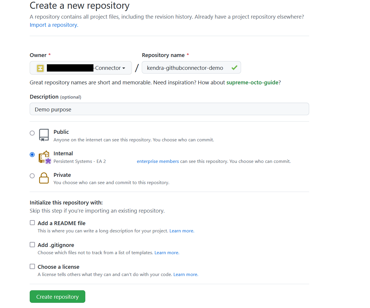
1. Create a new repository, and specify its owner and name.
2. Choose if the repository is public, internal, or private.
   
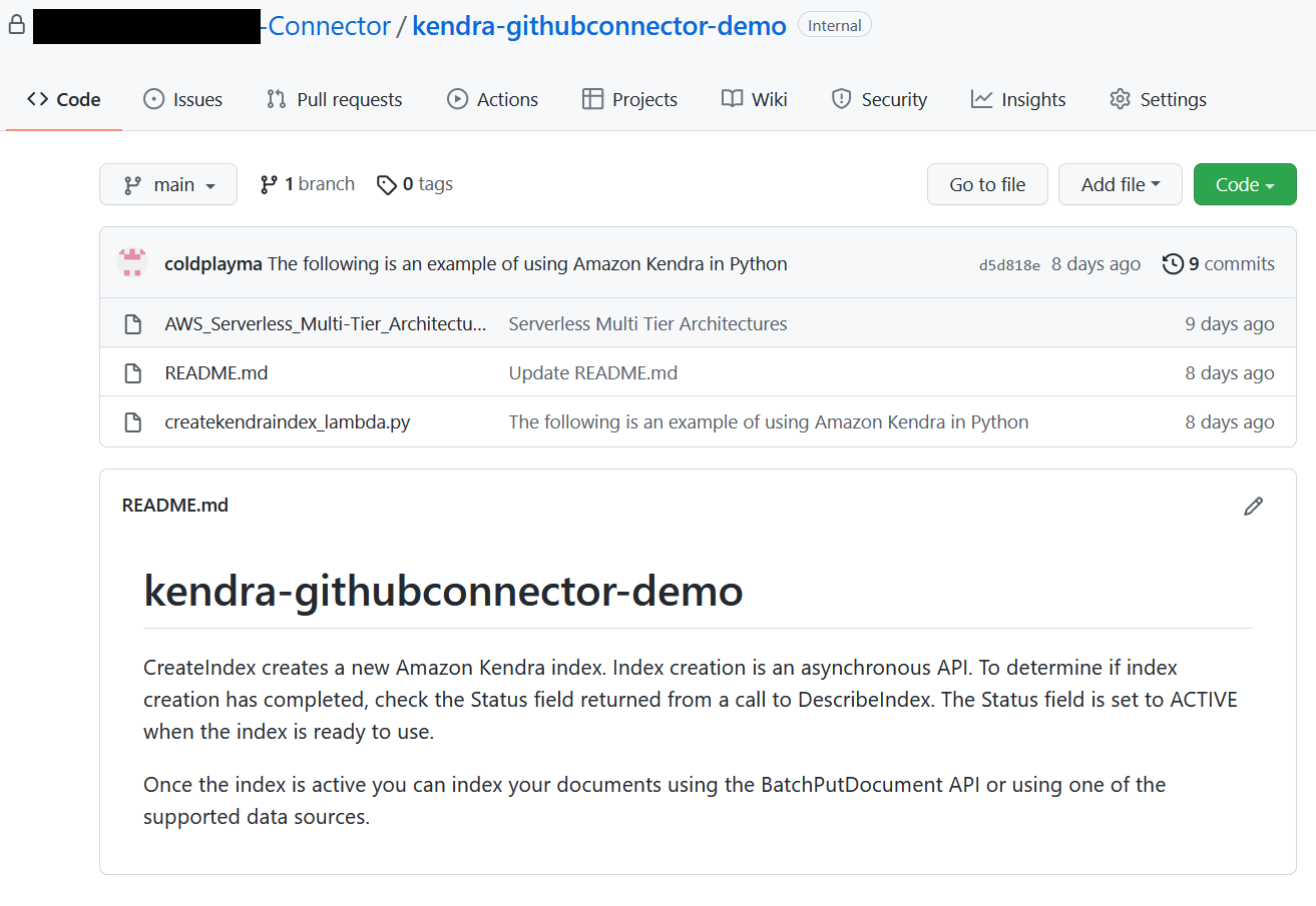
3. For this post, update the README file with the following text:

   CreateIndex API creates a new Amazon Kendra index. Index creation is an asynchronous API. To determine if index creation has completed, check the Status field returned from a call to DescribeIndex. The Status field is set to ACTIVE when the index is ready to use.
   Once the index is active you can index your documents using the BatchPutDocument API or using one of the supported data sources.

4. You can add a sample file to your repository with commit changes. The following is an example of using Amazon Kendra in Python:

   import boto3
   from botocore.exceptions import ClientError
   import pprint
   import time
   
   kendra = boto3.client("kendra")
   
   print("Create an index.")
   
   # Provide a name for the index
   index_name = "python-getting-started-index"
   # Provide an optional decription for the index
   description = "Getting started index"
   # Provide the IAM role ARN required for indexes
   index_role_arn = "arn:aws:iam::${accountId}:role/KendraRoleForGettingStartedIndex"
   
   try:
       index_response = kendra.create_index(
           Description = description,
           Name = index_name,
           RoleArn = index_role_arn
       )
   
       pprint.pprint(index_response)
   
       index_id = index_response["Id"]
   
       print("Wait for Amazon Kendra to create the index.")
   
       while True:
           # Get the details of the index, such as the status
           index_description = kendra.describe_index(
               Id = index_id
           )
           # When status is not CREATING quit.
           status = index_description["Status"]
           print(" Creating index. Status: "+status)
           time.sleep(60)
           if status != "CREATING":
               break
   
       print("Create an S3 data source.")
       
       # Provide a name for the data source
       data_source_name = "python-getting-started-data-source"
       # Provide an optional description for the data source
       data_source_description = "Getting started data source."
       # Provide the IAM role ARN required for data sources
       data_source_role_arn = "arn:aws:iam::${accountId}:role/KendraRoleForGettingStartedDataSource"
       # Provide the data source connection information 
       S3_bucket_name = "S3-bucket-name"
       data_source_type = "S3"
       # Configure the data source
       configuration = {"S3Configuration":
           {
               "BucketName": S3_bucket_name
           }
       }
   
       data_source_response = kendra.create_data_source(
           Name = data_source_name,
           Description = description,
           RoleArn = data_source_role_arn,
           Type = data_source_type,
           Configuration = configuration,
           IndexId = index_id
       )
   
       pprint.pprint(data_source_response)
   
       data_source_id = data_source_response["Id"]
   
       print("Wait for Amazon Kendra to create the data source.")
   
       while True:
           # Get the details of the data source, such as the status
           data_source_description = kendra.describe_data_source(
               Id = data_source_id,
               IndexId = index_id
           )
           # If status is not CREATING, then quit
           status = data_source_description["Status"]
           print(" Creating data source. Status: "+status)
           time.sleep(60)
           if status != "CREATING":
               break
   
       print("Synchronize the data source.")
   
       sync_response = kendra.start_data_source_sync_job(
           Id = data_source_id,
           IndexId = index_id
       )
   
       pprint.pprint(sync_response)
   
       print("Wait for the data source to sync with the index.")
   
       while True:
   
           jobs = kendra.list_data_source_sync_jobs(
               Id = data_source_id,
               IndexId = index_id
           )
   
           # For this example, there should be one job
           status = jobs["History"][0]["Status"]
   
           print(" Syncing data source. Status: "+status)
           if status != "SYNCING":
               break
           time.sleep(60)
   
   except  ClientError as e:
           print("%s" % e)
   
   print("Program ends.")

5. Download AWS_Whitepapers.zip to your computer, and extract the files into a folder called AWS_Whitepapers.
6. Upload AWS_Whitepapers/Best_Practices/AWS_Serverless_Multi-Tier_Architectures to your repository.

Your repository should look like the following screenshot.

Your organization’s code repositories might hold hundreds of thousands of documents, README notes, code comments, webpages, and other items. In the next section, we showcase the document comprehension capability of Amazon Kendra to find the relevant information contained in these repositories.

Create a GitHub data source connector

For this post, we assume you have already created an Amazon Kendra index. If you don’t have an index, create a new index before proceeding with the following steps.

1. On the Amazon Kendra console, choose the index that you want to add the data source to.
2. Choose Add data sources.
3. From the list of data source connectors, choose Add connector under GitHub.
   
4. On the Specify data source details page, enter a data source name and an optional description.
5. To assign metadata to your AWS resources in the form of tags, choose Add tags and enter a key and value.
6. Choose Next.
   
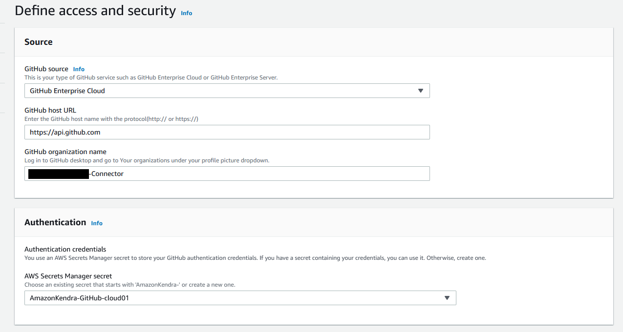
7. On the Define access and security page, choose your GitHub source. Amazon Kendra supports two types of GitHub services:
   1. GitHub Enterprise Cloud – If you choose this option, specify the GitHub host URL and GitHub organization name. Configure your Secrets Manager secret with the authentication credentials in the form of an OAuth2 access token of the GitHub enterprise owner. The Oauth2 token scope should be authorized for repo:status, public_repo, repo:invite, read:org, user:email, and read:user.
      
   2. GitHub Enterprise Server – If you choose this option, specify the GitHub host URL and GitHub organization name you created in the previous section. Configure your Secrets Manager secret with the authentication credentials in the form of an OAuth2 access token of the GitHub enterprise owner. The Oauth2 token scope should be authorized for repo:status, public_repo, repo:invite, read:org, user:email, read:user, and site_admin. To configure the SSL certificate, you can create a self-signed certificate for this post using openssl x509 -in sample.pem -out new_github.cer and add this certificate to an S3 bucket.
      
8. For Virtual Private Cloud (VPC), choose the default option (No VPC).
9. For IAM role, choose Create a new role (recommended) and enter a role name.
   Whenever you modify the Secrets Manager secret, make sure you also modify the IAM role, because it requires permission to access your secret to authenticate your GitHub account. For more information on the required permissions to include in the IAM role, see IAM roles for data sources.
10. Choose Next.
    
    On the Configure sync settings page, you provide details about the sync scope and run schedule.
11. For Select repositories to crawl, select Select repositories to configure a specific list.
12. Choose the repository kendra-githubconnector-demo that you created earlier.
13. Optionally, you can adjust the crawl mode. The GitHub connector supports the two modes:
    1. Full crawl mode – It crawls the entire GitHub organization as configured whenever there is a data source sync. By default, the connector runs in this mode.
    2. Change log mode – It crawls the specified changed GitHub content (added, deleted, modified, permission changes) of the organization whenever there is a data source sync.
14. Optionally, you can filter on the specific content types to index, and configure inclusion and exclusion filters on the file name, type, and path.
    
15. Under Sync run schedule, for Frequency, choose Run on demand.
16. Choose Next.
    
17. In the Set fields mapping section, define the mappings between GitHub fields to Amazon Kendra field names.
    You can configure for each content type and enable these GitHub fields as facets to further refine your search results. For this post, we use the default options.
18. Choose Next.
    
19. On the Review and create page, review your options for the GitHub data source.
20. Choose Add data source.
21. After the data source is created, choose Sync now to index the data from GitHub.

Search indexed content

After about 10 minutes, the data source sync is complete and the GitHub content is ingested into the index. The GitHub connector crawls the following entities:

• Repositories on GitHub Enterprise Cloud:
  • Repository with its description
  • Code and their branches with folders and subfolders
  • Issues and pull request files for public repositories
  • Issues and pull request comments and their replies for public and private repositories
  • Issues and pull request comment attachments and their replies’ attachments for public repositories
• Repositories on GitHub Enterprise Server:
  • Repository with its description
  • Code and their branches with folders and subfolders
  • Issues and pull request comments and their replies for public, private, and internal repositories

Now you can test some queries on the Amazon Kendra Search console.

1. Choose Search indexed content.
2. Enter the sample text How to check the status of the index creation?
   
3. Run another query and enter the sample text What are most popular usecases for AWS Lambda?
   

Amazon Kendra accurately surfaces relevant information based on the content indexed from the GitHub repositories. Access control to all the information is still enforced by the original repository.

Clean up

To avoid incurring unnecessary charges, clean up the resources you created for testing this connector.

1. Delete the Amazon Kendra index if you created one specifically for testing this solution.
2. Delete the GitHub connector data source if you added a new data source to an existing index.
3. Delete the content you added for your GitHub account.

Conclusion

In this post, we covered the process of setting up the new Amazon Kendra connector for GitHub. Organizations can empower their software developers by providing secure and intelligent search of content spread across many different GitHub repositories.

This post illustrates the basic connector capabilities. You can also customize the search by enabling facets based on GitHub fields and map to Amazon Kendra index fields. With the GitHub connector, you can control access to the data because it can crawl orgname-reponame and set a group as the principle and collaborators of the repository as members of the group. Furthermore, Amazon Kendra provides features such as Custom Document Enrichment and Experience Builder to enhance the search experience.

For more details about Amazon Kendra, refer to the Amazon Kendra Developer Guide.

About the Authors

Manjula Nagineni is a Solutions Architect with AWS based in New York. She works with major Financial service institutions, architecting, and modernizing their large-scale applications while adopting AWS cloud services. She is passionate about designing big data workloads cloud-natively. She has over 20 years of IT experience in Software Development, Analytics and Architecture across multiple domains such as finance, manufacturing and telecom.

Arjun Agrawal is Software Development Engineer at AWS Kendra.

Read More

Financial documents such as bank, loan, or mortgage statements are often formatted to be visually appealing and easy to read for the human eye. These same features can also make automated processing challenging at times. For instance, in the following sample statement, merging rows or columns in a table helps reduce information redundancy, but it can become difficult to write the code that identifies the repeating value and assign it to the corresponding elements.

In April 2022, Amazon Textract introduced a new capability of the table feature that automatically detects merged rows and columns as well as headers. Prior to this enhancement, for a similar document, the table’s output would have contained empty values for the Date column. Customers had to write custom code to detect the beginning of a new row and carry over the appropriate value.

This post walks you through a simple example of how to use the merged cells and headers features.

The new Amazon Textract table response structure

The response schema for the Amazon Textract API is now enhanced with two new structure types, as illustrated in the following diagram:

• A new block type called MERGED_CELL
• New cell entity types called COLUMN_HEADER or ROW_HEADER

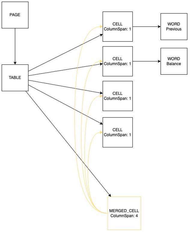
MERGED_CELL blocks are appended to the JSON document as any other CELL block. The MERGED_CELL blocks have a parent/child relationship with the CELL blocks they combine. This allows you to propagate the same cell value across multiple columns or rows even when not explicitly represented in the document. The MERGED_CELL block itself is then referenced from the TABLE block via a parent/child relationship.

Headers are flagged through a new entity type populated within the corresponding CELL block.

Using the new feature

Let’s try out the new feature on the sample statement presented earlier. The following code snippet calls Amazon Textract to extract tables out of the document, turn the output data into a Pandas DataFrame, and display its content.

We use the following modules in this example:

• amazon-textract-caller to invoke the Amazon Textract API on our behalf
• amazon-textract-response-parser to parse the response payload
• amazon-textract-prettyprinter to pretty-print tables

Let’s initialize the Boto3 session and invoke Amazon Textract with the sample statement as the input document:

session = boto3.Session(profile_name='<your_profile_name>')
documentName = " s3://amazon-textract-public-content/blogs/Textract-MergeCell-Sample-Bank-Statement.pdf"
textract_json = call_textract(input_document=documentName, features = [Textract_Features.TABLES])

Let’s pretty-print the response payload. As you can see, by default the date is not populated across all rows.

print(get_string(textract_json=textract_json, output_type=[Textract_Pretty_Print.TABLES]))

|--------------------|---------|
| Beginning Balance: | $8000.0 |
| Deposits           | $3005.5 |
| Other Subtractions | -1539.5 |
| Checks             |         |
| 0.00               |         |
| Service Fees 0.00  |         |

|-----------|----------|------------------------------|
| Account   | name     | John Doe                     |
| Account   | number   | 00002134001                  |
| Statement | Date:    |                              |
| Date      | February | 1, 2022 to February 28, 2022 |

|----------|-------------------------|---------|---------|--------|----------|
|          |                         |         | Amount  |        |          |
| Date     | Description             | Details | Credits | Debits | Balance  |
| 2/4/2022 | Life Insurance Payments | Credit  |         | 445    | 9500.45  |
|          | Property Management     | Credit  |         | 300    | 9945.45  |
|          | Retail Store 4          | Credit  |         | 65.75  | 10245.45 |
| 2/3/2022 | Electricity Bill        | Credit  |         | 245.45 | 10311.2  |
|          | Water Bill              | Credit  |         | 312.85 | 10556.65 |
|          | Rental Deposit          | Credit  | 3000    |        | 10869.5  |
| 2/2/2022 | Retail Store 3          | Credit  |         | 125    | 7869.5   |
|          | Retail Store 2 Refund   | Debit   | 5.5     |        | 7994.5   |
|          | Retail Store 1          | Credit  |         | 45.5   | 8000     |
| 2/1/2022 | Shoe Store Refund       | Credit  | 33      |        | 8045.5   |
|          | Snack Vending Machine   | Debit   |         | 4      | 8012.5   |

Then, we load the response into a document by using the Amazon Textract response parser module, and reorder the blocks by location:

t_doc = TDocumentSchema().load(textract_json)
ordered_doc = order_blocks_by_geo(t_doc)
trp_doc = Document(TDocumentSchema().dump(ordered_doc))

Now let’s iterate through the tables’ content, and extract the data into a DataFrame:

table_index = 1
dataframes = []
 def combine_headers(top_h, bottom_h):
   bottom_h[3] = top_h[2] + " " + bottom_h[3]
   bottom_h[4] = top_h[2] + " " + bottom_h[4]
 for page in trp_doc.pages:
   for table in page.tables:
     table_data = []
     headers = table.get_header_field_names()         #New Table method to retrieve header column names
     if(len(headers)>0):                   #Let's retain the only table with headers
       print("Statememt headers: "+ repr(headers))
       top_header= headers[0]
       bottom_header = headers[1]
       combine_headers(top_header, bottom_header)     #The statement has two headers. let's combine them
       for r, row in enumerate(table.rows_without_header): #New Table attribute returning rows without headers
         table_data.append([])
         for c, cell in enumerate(row.cells):
           table_data[r].append(cell.mergedText)    #New Cell attribute returning merged cells common values
       if len(table_data)>0:
         df = pd.DataFrame(table_data, columns=bottom_header)

The trp module has been improved to include two new capabilities, as highlighted in the preceding code’s comments:

• Fetch the header column names
• Expose merged cells’ repeated value

Displaying the DataFrame produces the following output.

We can now use multi-level indexing and reproduce the table’s initial structure:

multi = df.set_index(['Date', 'Details'])
display(multi)

For a complete version of the notebook presented in this post, visit the amazon-textract-code-samples GitHub repository.

Conclusion

Amazon Textract already helps you speed up document processing and reduce the number of manual tasks. The table’s new headers and merged cells features help you even further by reducing the need for custom or hard-coded logic. It can also help reduce postprocessing manual corrections.

For more information, please visit the Amazon Textract Response Objects documentation page. And if you are interested in learning more about another recently announced Textract feature, we highly recommend checking out Specify and extract information from documents using the new Queries feature in Amazon Textract.

About the Authors

Narcisse Zekpa is a Solutions Architect based in Boston. He helps customers in the Northeast U.S. accelerate their adoption of the AWS Cloud, by providing architectural guidelines, design innovative, and scalable solutions. When Narcisse is not building, he enjoys spending time with his family, traveling, cooking, and playing basketball.

Martin Schade is a Senior ML Product SA with the Amazon Textract team. He has over 20 years of experience with internet-related technologies, engineering, and architecting solutions. He joined AWS in 2014, first guiding some of the largest AWS customers on the most efficient and scalable use of AWS services, and later focused on AI/ML with a focus on computer vision. Currently, he’s obsessed with extracting information from documents.

Read More

Fraud plagues many online businesses and costs them billions of dollars each year. Financial fraud, counterfeit reviews, bot attacks, account takeovers, and spam are all examples of online fraud and malicious behaviors.

Although many businesses take approaches to combat online fraud, these existing approaches can have severe limitations. First, many existing methods aren’t sophisticated or flexible enough to detect the whole spectrum of fraudulent or suspicious online behaviors. Second, fraudsters can evolve and adapt to deceive simple rule-based or feature-based methods. For instance, fraudsters can create multiple coordinated accounts to avoid triggering limits on individual accounts.

However, if we construct a full interaction graph encompassing not only single transaction data but also account information, historical activities, and more, it’s more difficult for fraudsters to conceal their behavior. For example, accounts that are often connected to other fraudulent-related nodes may indicate guilt by association. We can also combine weak signals from individual nodes to derive stronger signals about that node’s activity. Fraud detection with graphs is effective because we can detect patterns such as node aggregation, which may occur when a particular user starts to connect with many other users or entities, and activity aggregation, which may occur when a large number of suspicious accounts begin to act in tandem.

In this post, we show you how to quickly deploy a financial transaction fraud detection solution with Graph Neural Networks (GNNs) using Amazon SageMaker JumpStart.

Alternatively, if you are looking for a fully managed service to build customized fraud detection models without writing code, we recommend checking out Amazon Fraud Detector. Amazon Fraud Detector enables customers with no machine learning experience to automate building fraud detection models customized for their data, leveraging more than 20 years of fraud detection expertise from Amazon Web Services (AWS) and Amazon.com.

Benefits of Graph Neural Networks

To illustrate why a Graph Neural Network is a great fit for online transaction fraud detection, let’s look at the following example heterogeneous graph constructed from a sample dataset of typical financial transaction data.

A heterogeneous graph contains different types of nodes and edges, which in turn tend to have different types of attributes that are designed to capture characteristics of each node and edge type.

The sample dataset contains not only features of each transaction, such as the purchased product type and transaction amount, but also multiple identity information that could be used to identify the relations between transactions. That information can be used to construct Relational Graph Convolutional Networks (R-GCNs). In the preceding example graph, the node types correspond to categorical columns in the sample dataset such as card number, card type, and email domain.

GNNs utilize all the constructed information to learn a hidden representation (embedding) for each transaction, so that the hidden representation is used as input for a linear classification layer to determine whether the transaction is fraudulent or not.

The solution shown in this post uses Amazon SageMaker and the Deep Graph Library (DGL) to construct a heterogeneous graph from tabular data and train an R-GCNs model to identify fraudulent transactions.

Solution overview

At a high level, the solution trains a graph neural network to accept an interaction graph, as well as some features about the users in order to classify those users as potentially fraudulent or not. This approach ensures that we detect signals that are present in the user attributes or features, as well as in the connectivity structure, and interaction behavior of the users.

This solution employs the following algorithms:

• R-GCNs, which is a state-of-the-art GNN model for heterogenous graph input
• SageMaker XGBoost, which we use as the baseline model to compare performances

By default, this solution uses synthetic datasets that are created to mimic typical examples of financial transactions datasets. We demonstrate how to use your own labeled dataset later in this post.

The outputs of the solution are as follows:

• An R-GCNs model trained on the input datasets.
• An XGBoost model trained on the input datasets.
• Predictions of the probability for each transaction being fraudulent. If the estimated probability of a transaction is over a threshold, it’s classified as fraudulent.

In this solution, we focus on the SageMaker components, which include two main parts:

• The first part uses SageMaker Processing to do feature engineering and extract edge lists from a table of transactions or interactions
• The second part uses SageMaker training infrastructure to train the models for fraud detection, including an XGBoost baseline model, and a GNN model with the DGL

The following diagram illustrates the solution architecture.

Prerequisites

To try out the solution in your own account, make sure that you have the following in place:

• You need an AWS account to use this solution. If you don’t have an account, you can sign up for one.
• The solution outlined in this post is part of JumpStart. To run this JumpStart 1P Solution and have the infrastructure deploy to your AWS account, you need to create an active Amazon SageMaker Studio instance (see Onboard to Amazon SageMaker Domain).

When the Studio instance is ready, you can launch Studio and access JumpStart. JumpStart solutions are not available in SageMaker notebook instances, and you can’t access them through SageMaker APIs or the AWS Command Line Interface (AWS CLI).

Launch the solution

To launch the solution, complete the following steps:

1. Open JumpStart by using the JumpStart launcher in the Get Started section or by choosing the JumpStart icon in the left sidebar.
2. Under Solutions, choose Fraud Detection in Financial Transactions to open the solution in another Studio tab.
   
3. In the solution tab, choose Launch to launch the solution.
   
   The solution resources are provisioned and another tab opens showing the deployment progress. When the deployment is finished, an Open Notebook button appears.
4. Choose Open Notebook to open the solution notebook in Studio.
   

Explore the default dataset

The default dataset used in this solution is a synthetic dataset created to mimic typical examples of financial transactions dataset that many companies have. The dataset consists of two tables:

• Transactions – Records transactions and metadata about transactions between two users. Examples of columns include the product code for the transaction and features on the card used for the transaction, and a column indicating whether the corresponded transaction is fraud or not.
• Identity – Contains information about the identity users performing transactions. Examples of columns include the device type and device IDs used.

The two tables can be joined together using the unique identified-key column TransactionID. The following screenshot shows the first five observations of the Transactions dataset.

The following screenshot shows the first five observations of the Identity dataset.

The following screenshot shows the joined dataset.

Besides the unique identifier column (TransactionID) to identify each transaction, there are two types of predicting columns and one target column:

• Identity columns – These contain identity information related to a transaction, including card_no, card_type, email_domain, IpAddress, PhoneNo, and DeviceID
• Categorical or numerical columns – These describe the features of each transaction, including ProductCD and TransactionAmt
• Target column – The isFraud column indicates whether the corresponded transaction is fraudulent or not

The goal is to fully utilize the information in the predicting columns to classify each transaction (each row in the table) to be either fraud or not fraud.

Upload the raw data to Amazon S3

The solution notebook contains code that downloads the default synthetic datasets and uploads them to the input Amazon Simple Storage Service (Amazon S3) bucket provisioned by the solution.

To use your own labeled datasets, before running the code cell in the Upload raw data to S3 notebook section, edit the value of the variable raw_data_location so that it points to the location of your own input data.

In the Data Visualization notebook section, you can run the code cells to visualize and explore the input data as tables.

If you’re using your own datasets with different data file names or table columns, remember to also update the data exploration code accordingly.

Data preprocessing and feature engineering

The solution provides a data preprocessing and feature engineering Python script data-preprocessing/graph_data_preprocessor.py. This script serves as a general processing framework to convert a relational table to heterogeneous graph edge lists based on the column types of the relational table. Some of the data transformation and feature engineering techniques include:

• Performing numerical encoding for categorical variables and logarithmic transformation for transaction amount
• Constructing graph edge lists between transactions and other entities for the various relation types

All the columns in the relational table are classified into one of the following three types for data transformation:

• Identity columns – Columns that contain identity information related to a user or a transaction, such as IP address, phone number, and device identifiers. These column types become node types in the heterogeneous graph, and the entries in these columns become the nodes.
• Categorical columns – Columns that correspond to categorical features such as a user’s age group, or whether or not a provided address matches an address on file. The entries in these columns undergo numerical feature transformation and are used as node attributes in the heterogeneous graph.
• Numerical columns – Columns that correspond to numerical features such as how many times a user has tried a transaction. The entries here are also used as node attributes in the heterogeneous graph. The script assumes that all columns in the tables that aren’t identity columns or categorical columns are numerical columns.

The names of the identity columns and categorical columns need to be provided as command line arguments when running the Python script (--id-cols for identity column names and --cat-cols for category column names).

If you’re using your own data and your data is in the same format as the default synthetic dataset but with different column names, you simply need to adapt the Python arguments in the notebook code cell according to your dataset’s column names. However, if your data is in a different format, you need to modify the following section in the data-preprocessing/graph_data_preprocessor.py Python script.

We divide the dataset into training (70% of the entire data), validation (20%), and test datasets (10%). The validation dataset is used for hyperparameter optimization (HPO) to select the optimal set of hyperparameters. The test dataset is used for the final evaluation to compare various models. If you need to adjust these ratios, you can use the command line arguments --train-data-ratio and --valid-data-ratio when running the preprocessing Python script.

When the preprocessing job is complete, we have a set of bipartite edge lists between transactions and different device ID types (suppose we’re using the default dataset), as well as the features, labels, and a set of transactions to validate our graph model performance. You can find the transformed data in the S3 bucket created by the solution, under the dgl-fraud-detection/preprocessed-data folder.

Train an XGBoost baseline model with HPO

Before diving into training a graph neural network with the DGL, we first train an XGBoost model with HPO as the baseline on the transaction table data.

1. Read the data from features_xgboost.csv and upload the data to Amazon S3 for training the baseline model. This CSV file was generated in the data preprocessing and feature engineering job in the last step. Only the categorical columns productCD, card_type, and the numerical column TransactionAmt are included.
2. Create an XGBoost estimator with the SageMaker XGBoost algorithm container.
3. Create and fit an XGBoost estimator with HPO:
   1. Specify dynamic hyperparameters we want to tune and their searching ranges.
   2. Define optimization objectives in terms of metrics and objective type.
   3. Create hyperparameter tuning jobs to train the model.
4. Deploy the endpoint of the best tuning job and make predictions with the baseline model.

Train the Graph Neural Network using the DGL with HPO

Graph Neural Networks work by learning representation for nodes or edges of a graph that are well suited for some downstream tasks. We can model the fraud detection problem as a node classification task, and the goal of the GNN is to learn how to use information from the topology of the sub-graph for each transaction node to transform the node’s features to a representation space where the node can be easily classified as fraud or not.

Specifically, we use a relational graph convolutional neural networks model (R-GCNs) on a heterogeneous graph because we have nodes and edges of different types.

1. Define hyperparameters to determine properties such as the class of GNN models, the network architecture, the optimizer, and optimization parameters.
2. Create and train the R-GCNs model.

For this post, we use the DGL, with MXNet as the backend deep learning framework. We create a SageMaker MXNet estimator and pass in our model training script (sagemaker_graph_fraud_detection/dgl_fraud_detection/ train_dgl_mxnet_entry_point.py), the hyperparameters, as well as the number and type of training instances we want to use. When the training is complete, the trained model and prediction result on the test data are uploaded to Amazon S3.

1. Optionally, you can inspect the prediction results and compare the model metrics with the baseline XGBoost model.
2. Create and fit a SageMaker estimator using the DGL with HPO:
   1. Specify dynamic hyperparameters we want to tune and their searching ranges.
   2. Define optimization objectives in terms of metrics and objective type.
   3. Create hyperparameter tuning jobs to train the model.
3. Read the prediction output for the test dataset from the best tuning job.

Clean up

When you’re finished with this solution, make sure that you delete all unwanted AWS resources to avoid incurring unintended charges. In the Delete solution section on your solution tab, choose Delete all resources to delete resources automatically created when launching this solution.

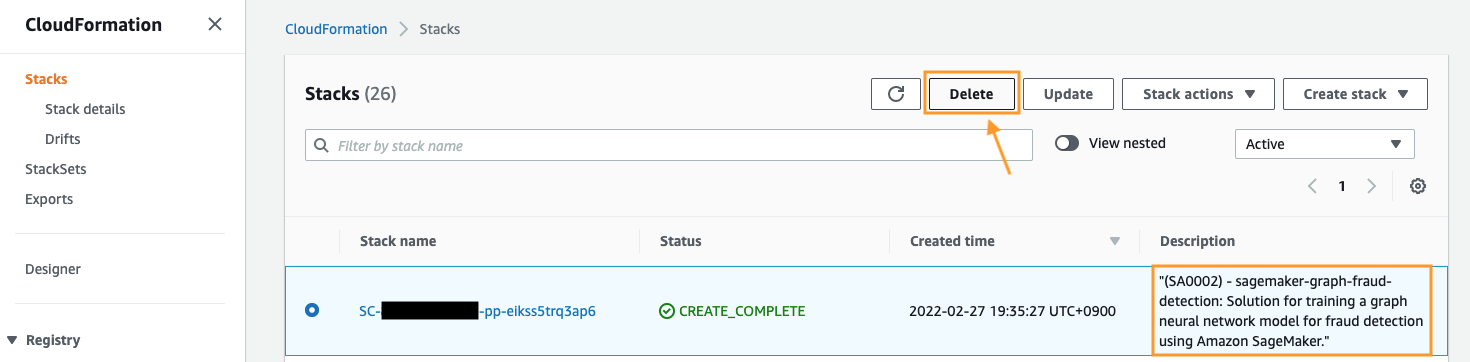
Alternatively, you can use AWS CloudFormation to delete all standard resources automatically created by the solution and notebook. To use this approach, on the AWS CloudFormation console, find the CloudFormation stack whose description contains sagemaker-graph-fraud-detection, and delete it. This is a parent stack; deleting this stack automatically deletes the nested stacks.

With either approach, you still need to manually delete any extra resources that you may have created in this notebook. Some examples include extra S3 buckets (in addition to the solution’s default bucket), extra SageMaker endpoints (using a custom name), and extra Amazon Elastic Container Registry (Amazon ECR) repositories.

Conclusion

In this post, we discussed the business problem caused by online transaction fraud, the issues in traditional fraud detection approaches, and why a GNN is a good fit for solving this business problem. We showed you how to build an end-to-end solution for detecting fraud in financial transactions using a GNN with SageMaker and a JumpStart solution. We also explained other features of JumpStart, such as using your own dataset, using SageMaker algorithm containers, and using HPO to automate hyperparameter tuning and find the best tuning job to make predictions.

To learn more about this JumpStart solution, check out the solution’s GitHub repository.

About the Authors

Xiaoli Shen is a Solutions Architect and Machine Learning Technical Field Community (TFC) member at Amazon Web Services. She’s focused on helping customers architecting on the cloud and leveraging AWS services to derive business value. Prior to joining AWS, she was a senior full-stack engineer building large-scale data-intensive distributed systems on the cloud. Outside of work she’s passionate about volunteering in technical communities, traveling the world, and making music.

Dr. Xin Huang is an applied scientist for Amazon SageMaker JumpStart and Amazon SageMaker built-in algorithms. He focuses on developing scalable machine learning algorithms. His research interests are in the area of natural language processing, explainable deep learning on tabular data, and robust analysis of non-parametric space-time clustering.

Vedant Jain is a Sr. AI/ML Specialist Solutions Architect, helping customers derive value out of the Machine Learning ecosystem at AWS. Prior to joining AWS, Vedant has held ML/Data Science Specialty positions at various companies such as Databricks, Hortonworks (now Cloudera) & JP Morgan Chase. Outside of his work, Vedant is passionate about making music, using Science to lead a meaningful life & exploring delicious vegetarian cuisine from around the world.

Read More

Having an environment capable of delivering Amazon SageMaker notebook instances quickly allows data scientists and business analysts to efficiently respond to organizational needs. Data is the lifeblood of an organization, and analyzing that data efficiently provides useful insights for businesses. A common issue that organizations encounter is creating an automated pattern that enables development teams to launch AWS services. Organizations want to enable their developers to launch resources as they need them, but in a centralized and secure fashion.

This post demonstrates how to centralize the management of SageMaker instance notebooks using AWS services including AWS CloudFormation, AWS Serverless Application Model (AWS SAM), AWS Service Catalog, Amazon EventBridge, AWS Systems Manager Parameter Store, Amazon API Gateway, and AWS Lambda. We walk through how to use these AWS services to automate the process of vending SageMaker notebooks to end-users.

Solution overview

In our solution, a notebook user requests a notebook instance using AWS Service Catalog. The request is processed by AWS CloudFormation, which delivers the notebook instance. EventBridge monitors the AWS Service Catalog API for completion of the notebook instance resource provisioning. An event-based rule in EventBridge calls the Lambda event processor, which runs a Lambda function returning the presigned URL.

The following architectural diagram illustrates the infrastructure state as defined in the CloudFormation templates.

The process consists of the following steps:

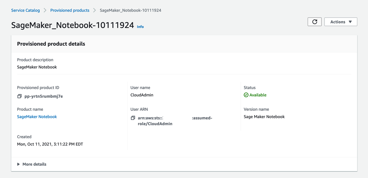
1. A user requests a new notebook via the AWS Service Catalog console.
2. AWS Service Catalog launches a CloudFormation stack.
3. AWS CloudFormation launches the SageMaker notebook.
4. A SageMaker notebook is now running.
5. An EventBridge function is triggered when a new AWS Service Catalog product is launched.
6. The Amazon CloudWatch event invokes a Lambda function that generates the presigned URL and a user-specific SSM parameter.
7. A user requests a new presigned URL.
8. A Lambda function generates a new presigned URL and updates the user’s SSM parameter with the new URL.

Prerequisites

To implement this solution, you must have the following prerequisites:

• An AWS account with local credentials properly configured (typically under ~/.aws/credentials).
• An AWS Identity and Access Management (IAM) role configured with administrative privileges.
• The latest version of the AWS Command Line Interface (AWS CLI). For more information, refer to Installing or updating the latest version of the AWS CLI.
• A Git client to clone the source code located here.
• The latest version of the AWS SAM CLI.

Deploy resources with AWS CloudFormation

To create your resources with AWS CloudFormation, complete the following steps:

1. Deploy the s3-iam-config CloudFormation template:

   aws cloudformation create-stack 
   --stack-name s3-iam-config 
   --template-body file://templates/s3-iam-config.yml 
   --parameters file://parameters/s3-iam-params.json 
   --capabilities CAPABILITY_NAMED_IAM

The output should look like the following code:

{
"StackId": "arn:aws:cloudformation:us-east-1:123456789012:stack/s3-iam-config/9be9f990-0909-11eb-811c-0a78092beb51"
}

The template creates an Amazon Simple Storage Service (Amazon S3) bucket.

2. Run the following command to get the S3 bucket name generated in the previous step:

   aws cloudformation describe-stacks 
   --stack-name s3-iam-config 
   --query "Stacks[0].Outputs[?OutputKey=='S3BucketName'].OutputValue" 
   --output text

The output should look like the following:

s3-iam-config-s3bucket-1p85zr5051d86

3. Run the following command using the output from the previous step (update the bucket name):

   aws s3 cp templates/sm-notebook.yml s3://<bucket_name>/sm-notebook.yml

The output should look like the following:

upload: templates/sm-notebook.yml to s3://s3-iam-config-s3bucket-1p85zr5051d86/sm-notebook.yml

4. Open the parameters/service-catalog-params.json file and update the S3BucketName parameter to the bucket name from the previous step. Update the UserIAMPrincipal with the ARN of the IAM role you’re using for this demo.

   [
     {
       "ParameterKey" : "NotebookInstanceType",
       "ParameterValue" : "ml.t2.medium"
     },
     {
       "ParameterKey" : "S3IAMConfigStackName",
       "ParameterValue" : "s3-iam-config"
     },
     {
       "ParameterKey" : "ServiceCatalogTemplateName",
       "ParameterValue" : "sm-notebook.yml"
     },
     {
       "ParameterKey" : "S3BucketName",
       "ParameterValue" : "<input_your_bucket_name>"
     },
     {
       "ParameterKey" : "UserIAMPrincipal",
       "ParameterValue" : "<input_your_iam_principal_arn>"
     }
   ]

5. Deploy the service-catalog CloudFormation template:

   aws cloudformation create-stack 
   --stack-name service-catalog-config 
   --template-body file://templates/service-catalog.yml 
   --parameters file://parameters/service-catalog-params.json 
   --capabilities CAPABILITY_NAMED_IAM

The output should look like the following:

{
    "StackId": "arn:aws:cloudformation:us-east-1:123456789012:stack/service-catalog-config/fb29c5e0-28a0-11ec-8337-123f746ae8a3"
}

Deploy resources with AWS SAM

To deploy resources with AWS SAM, complete the following steps:

1. Change your directory to the lambda directory:

   cd lambda/

2. Build the application:

   sam build

The output should look like the following:

Built Artifacts  : .aws-sam/build
Built Template   : .aws-sam/build/template.yaml

Commands you can use next
=========================
[*] Invoke Function: sam local invoke
[*] Test Function in the Cloud: sam sync --stack-name {stack-name} --watch
[*] Deploy: sam deploy --guided

3. Deploy the application:

   sam deploy --guided

4. Respond to the questions in the CLI as shown in the following code:

     Configuring SAM deploy
   ======================
   
           Looking for config file [samconfig.toml] :  Found
           Reading default arguments  :  Success
   
           Setting default arguments for 'sam deploy'
           =========================================
           Stack Name [sam-app]: sam-app
           AWS Region [us-east-1]: us-east-1
           Parameter EventBridgeFunctionName [EventBridgeFunction]: EventBridgeFunction
           Parameter EventRuleName [SvcCatalogEventRule]: SvcCatalogEventRule
           Parameter RefreshFunctionName [RefreshURLFunction]: RefreshURLFunction
           #Shows you resources changes to be deployed and require a 'Y' to initiate deploy
           Confirm changes before deploy [y/N]: N
           #SAM needs permission to be able to create roles to connect to the resources in your template
           Allow SAM CLI IAM role creation [Y/n]: Y
           #Preserves the state of previously provisioned resources when an operation fails
           Disable rollback [y/N]: N
           EventBridgeFunction may not have authorization defined, Is this okay? [y/N]: Y
           RefreshURLFunction may not have authorization defined, Is this okay? [y/N]: Y
           Save arguments to configuration file [Y/n]: Y
           SAM configuration file [samconfig.toml]: samconfig.toml
           SAM configuration environment [default]: dev

The output should look like the following:

        Looking for resources needed for deployment:
        Creating the required resources...
        Successfully created!
         Managed S3 bucket: aws-sam-cli-managed-default-samclisourcebucket-1f4i68wsmouhw
         A different default S3 bucket can be set in samconfig.toml

        Saved arguments to config file
        Running 'sam deploy' for future deployments will use the parameters saved above.
        The above parameters can be changed by modifying samconfig.toml
        Learn more about samconfig.toml syntax at 
        https://docs.aws.amazon.com/serverless-application-model/latest/developerguide/serverless-sam-cli-config.html

Uploading to sam-app/6f3e2f13cfdca08133238f77fc2c667b  9425988 / 9425988  (100.00%)
Uploading to sam-app/b153fd4be66b581361f7d46efae25f18  9425968 / 9425968  (100.00%)

        Deploying with following values
        ===============================
        Stack name                   : sam-app
        Region                       : us-east-1
        Confirm changeset            : False
        Disable rollback             : False
        Deployment s3 bucket         : aws-sam-cli-managed-default-samclisourcebucket-1f4i68wsmouhw
        Capabilities                 : ["CAPABILITY_IAM"]
        Parameter overrides          : {"EventBridgeFunctionName": "EventBridgeFunction", "EventRuleName": "SvcCatalogEventRule", "RefreshFunctionName": "RefreshURLFunction"}
        Signing Profiles             : {}

Initiating deployment
=====================
Uploading to sam-app/c82cdea2bfbc2abc6520a97fce4c8a8b.template  6754 / 6754  (100.00%)

Waiting for changeset to be created..

CloudFormation stack changeset
-----------------------------------------------------------------------------------------------------------------------------------------------------------------
Operation                                LogicalResourceId                        ResourceType                             Replacement                            
-----------------------------------------------------------------------------------------------------------------------------------------------------------------
+ Add                                    EventBridgeFunctionHelloWorldPermissio   AWS::Lambda::Permission                  N/A                                    
                                         nProd                                                                                                                    
+ Add                                    EventBridgeFunctionRole                  AWS::IAM::Role                           N/A                                    
+ Add                                    EventBridgeFunction                      AWS::Lambda::Function                    N/A                                    
+ Add                                    PermissionForEventsToInvokeLambda        AWS::Lambda::Permission                  N/A                                    
+ Add                                    RefreshURLFunctionHelloWorldPermission   AWS::Lambda::Permission                  N/A                                    
                                         Prod                                                                                                                     
+ Add                                    RefreshURLFunctionRole                   AWS::IAM::Role                           N/A                                    
+ Add                                    RefreshURLFunction                       AWS::Lambda::Function                    N/A                                    
+ Add                                    ServerlessRestApiDeploymentb762875163    AWS::ApiGateway::Deployment              N/A                                    
+ Add                                    ServerlessRestApiProdStage               AWS::ApiGateway::Stage                   N/A                                    
+ Add                                    ServerlessRestApi                        AWS::ApiGateway::RestApi                 N/A                                    
+ Add                                    SvcCatalogEventRule                      AWS::Events::Rule                        N/A                                    
-----------------------------------------------------------------------------------------------------------------------------------------------------------------

Changeset created successfully. arn:aws:cloudformation:us-east-1:123456789012:changeSet/samcli-deploy1641934511/763fe89c-9c6a-4cef-a1a6-90986d7decfd


2022-01-11 15:55:22 - Waiting for stack create/update to complete

CloudFormation events from stack operations
-----------------------------------------------------------------------------------------------------------------------------------------------------------------
ResourceStatus                           ResourceType                             LogicalResourceId                        ResourceStatusReason                   
-----------------------------------------------------------------------------------------------------------------------------------------------------------------
CREATE_IN_PROGRESS                       AWS::IAM::Role                           RefreshURLFunctionRole                   -                                      
CREATE_IN_PROGRESS                       AWS::IAM::Role                           EventBridgeFunctionRole                  -                                      
CREATE_IN_PROGRESS                       AWS::IAM::Role                           EventBridgeFunctionRole                  Resource creation Initiated            
CREATE_IN_PROGRESS                       AWS::IAM::Role                           RefreshURLFunctionRole                   Resource creation Initiated            
CREATE_COMPLETE                          AWS::IAM::Role                           EventBridgeFunctionRole                  -                                      
CREATE_IN_PROGRESS                       AWS::Lambda::Function                    EventBridgeFunction                      -                                      
CREATE_IN_PROGRESS                       AWS::Lambda::Function                    EventBridgeFunction                      Resource creation Initiated            
CREATE_COMPLETE                          AWS::IAM::Role                           RefreshURLFunctionRole                   -                                      
CREATE_COMPLETE                          AWS::Lambda::Function                    EventBridgeFunction                      -                                      
CREATE_IN_PROGRESS                       AWS::Lambda::Function                    RefreshURLFunction                       -                                      
CREATE_IN_PROGRESS                       AWS::Lambda::Function                    RefreshURLFunction                       Resource creation Initiated            
CREATE_IN_PROGRESS                       AWS::Events::Rule                        SvcCatalogEventRule                      -                                      
CREATE_IN_PROGRESS                       AWS::Events::Rule                        SvcCatalogEventRule                      Resource creation Initiated            
CREATE_COMPLETE                          AWS::Lambda::Function                    RefreshURLFunction                       -                                      
CREATE_IN_PROGRESS                       AWS::ApiGateway::RestApi                 ServerlessRestApi                        -                                      
CREATE_COMPLETE                          AWS::ApiGateway::RestApi                 ServerlessRestApi                        -                                      
CREATE_IN_PROGRESS                       AWS::ApiGateway::RestApi                 ServerlessRestApi                        Resource creation Initiated            
CREATE_IN_PROGRESS                       AWS::ApiGateway::Deployment              ServerlessRestApiDeploymentb762875163    -                                      
CREATE_IN_PROGRESS                       AWS::Lambda::Permission                  EventBridgeFunctionHelloWorldPermissio   -                                      
                                                                                  nProd                                                                           
CREATE_IN_PROGRESS                       AWS::Lambda::Permission                  RefreshURLFunctionHelloWorldPermission   Resource creation Initiated            
                                                                                  Prod                                                                            
CREATE_IN_PROGRESS                       AWS::Lambda::Permission                  EventBridgeFunctionHelloWorldPermissio   Resource creation Initiated            
                                                                                  nProd                                                                           
CREATE_IN_PROGRESS                       AWS::Lambda::Permission                  RefreshURLFunctionHelloWorldPermission   -                                      
                                                                                  Prod                                                                            
CREATE_IN_PROGRESS                       AWS::ApiGateway::Deployment              ServerlessRestApiDeploymentb762875163    Resource creation Initiated            
CREATE_COMPLETE                          AWS::ApiGateway::Deployment              ServerlessRestApiDeploymentb762875163    -                                      
CREATE_IN_PROGRESS                       AWS::ApiGateway::Stage                   ServerlessRestApiProdStage               -                                      
CREATE_IN_PROGRESS                       AWS::ApiGateway::Stage                   ServerlessRestApiProdStage               Resource creation Initiated            
CREATE_COMPLETE                          AWS::Lambda::Permission                  RefreshURLFunctionHelloWorldPermission   -                                      
                                                                                  Prod                                                                            
CREATE_COMPLETE                          AWS::Lambda::Permission                  EventBridgeFunctionHelloWorldPermissio   -                                      
                                                                                  nProd                                                                           
CREATE_COMPLETE                          AWS::ApiGateway::Stage                   ServerlessRestApiProdStage               -                                      
CREATE_COMPLETE                          AWS::Events::Rule                        SvcCatalogEventRule                      -                                      
CREATE_IN_PROGRESS                       AWS::Lambda::Permission                  PermissionForEventsToInvokeLambda        -                                      
CREATE_IN_PROGRESS                       AWS::Lambda::Permission                  PermissionForEventsToInvokeLambda        Resource creation Initiated            
CREATE_COMPLETE                          AWS::Lambda::Permission                  PermissionForEventsToInvokeLambda        -                                      
CREATE_COMPLETE                          AWS::CloudFormation::Stack               sam-app                                  -                                      
-----------------------------------------------------------------------------------------------------------------------------------------------------------------

CloudFormation outputs from deployed stack
------------------------------------------------------------------------------------------------------------------------------------------------------------------
Outputs                                                                                                                                                          
------------------------------------------------------------------------------------------------------------------------------------------------------------------
Key                 RefreshURLFunctionIamRole                                                                                                                    
Description         Implicit IAM Role created for Hello World function                                                                                           
Value               arn:aws:lambda:us-east-1:123456789012:function:RefreshURLFunction                                                                            

Key                 RefreshURLFunctionAPI                                                                                                                        
Description         API Gateway endpoint URL for Prod stage for Hello World function                                                                             
Value               https://m94bjaurjb.execute-api.us-east-1.amazonaws.com/Prod/refreshurl/                                                                      

Key                 RefreshURLFunction                                                                                                                           
Description         Hello World Lambda Function ARN                                                                                                              
Value               arn:aws:lambda:us-east-1:123456789012:function:RefreshURLFunction                                                                            
------------------------------------------------------------------------------------------------------------------------------------------------------------------

Successfully created/updated stack - sam-app in us-east-1

Test the solution

Now that you have deployed the solution, let’s test the workflow.

1. On the AWS Service Catalog console, under Administration in the navigation pane, choose Portfolios.
   
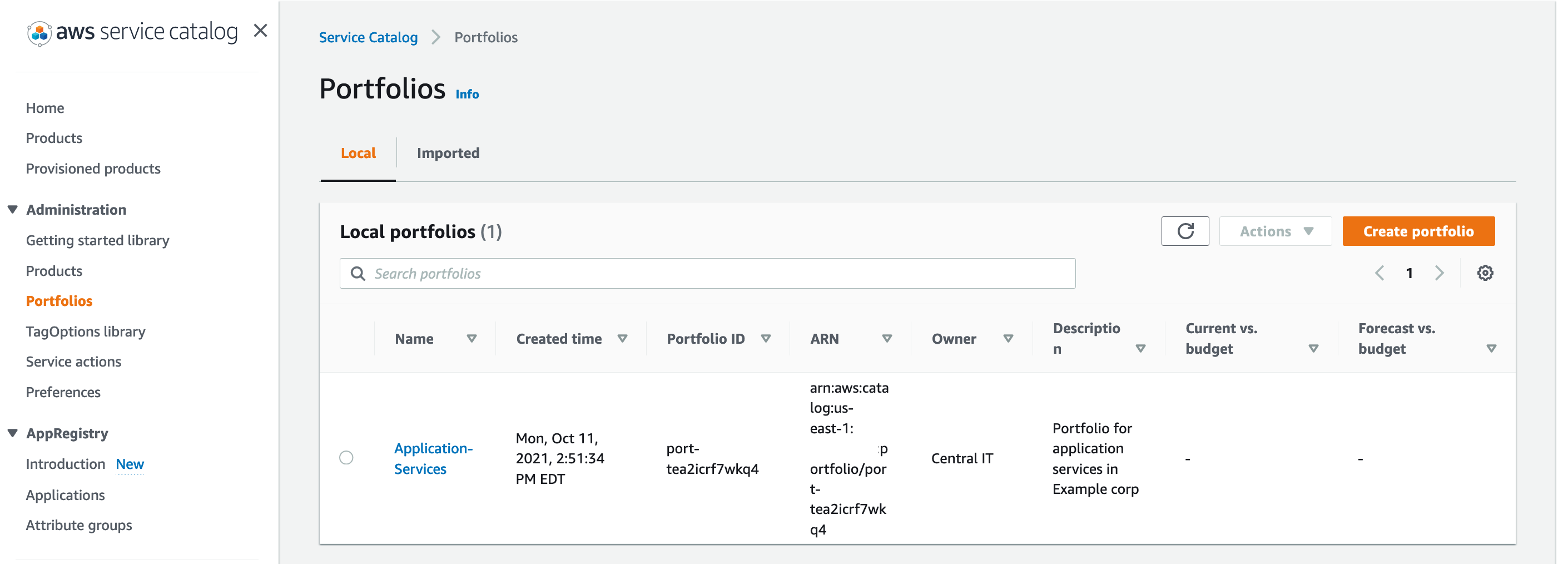
2. Choose your SageMaker notebook.
   
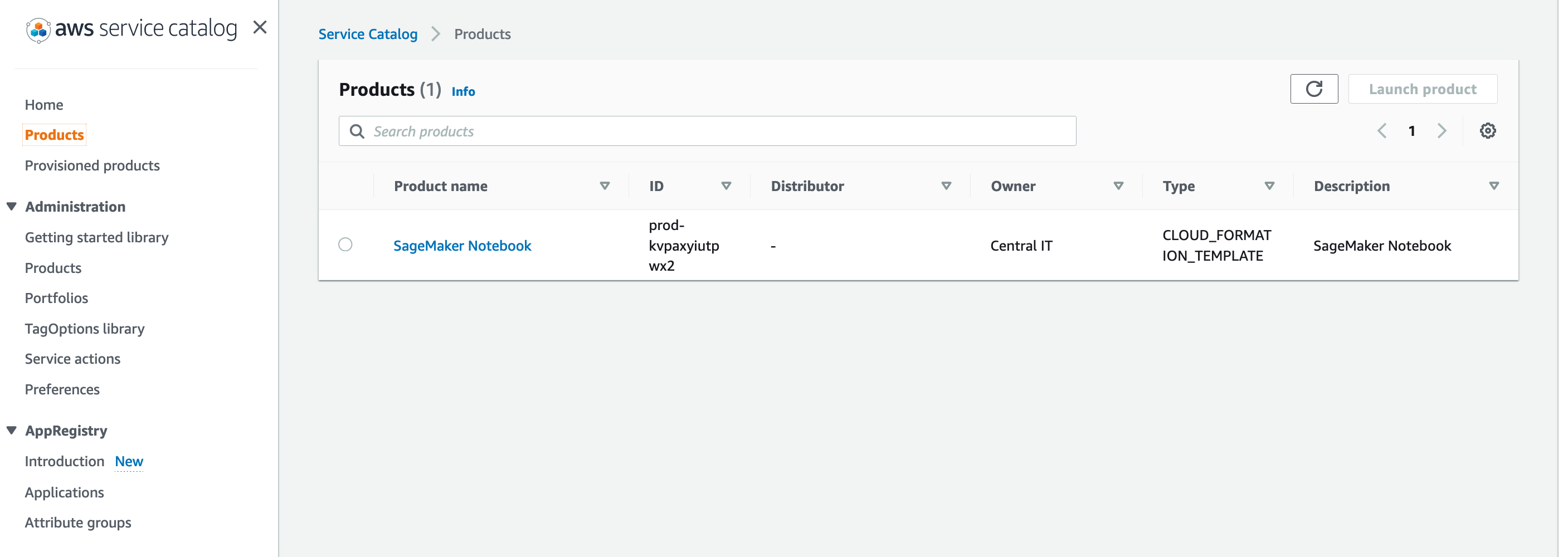
3. Choose Launch product.
   
4. At the bottom of the page, choose Launch product.
   

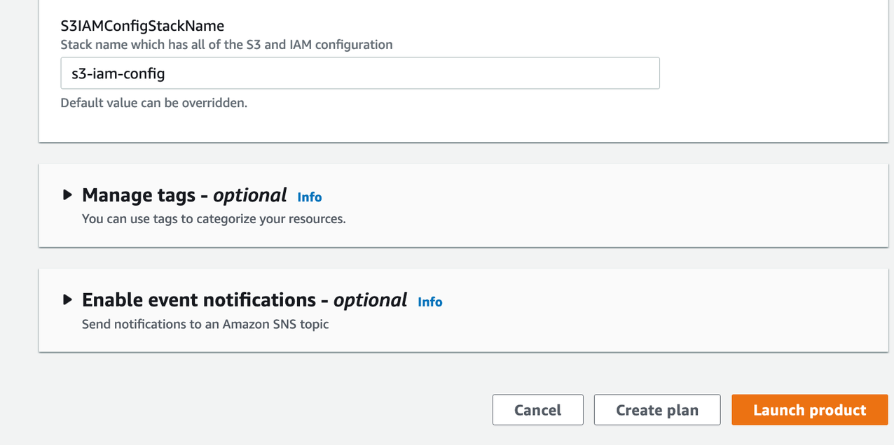
You should see a page similar to the following screenshot.

5. Wait a few moments for the status to show as Available.
   
6. Open your terminal and run the following command to get the presigned URL from Parameter Store:

   aws ssm get-parameter 
   --name "/SageMaker/Notebooks/Demo-User-Notebook" 
   --query Parameter.Value

The output should look like the following:

"https://demo-user-notebook.notebook.us-east-1.sagemaker.aws?authToken=eyJhbGciOiJIUzI1NiJ9.eyJmYXNDcmVkZW50aWFscyI6IkFZQURlSlVvLzJjeEcwQ0xtNHBjTTZFOGM1SUFYd0FCQUJWaGQzTXRZM0o1Y0hSdkxYQjFZbXhwWXkxclpYa0FSRUV3U0ZSdU1rNXJZMUpyWnpWWVlsZFBRbUowTmtadVpGcHZlRlJXUW05SVlWaHdiazFJY25WRWVrTmtlVWRUVUZsak56UnhObWQzVTJGS1dYUm5hVk40VVQwOUFBRUFCMkYzY3kxcmJYTUFTMkZ5YmpwaGQzTTZhMjF6T25WekxXVmhjM1F0TVRvM05qUTNNRGM1TWpRME1UVTZhMlY1TDJJM01ETTNNRE5oTFdVMU5HTXROR1JtWWkxaE1HRTFMVGMyTnpNek1XWXlORGsxT1FDNEFRSUJBSGhlY3J4TGdEdDJaWmRKYk5nd3R4RHJpWmtZQnZUR1cwZWZCWVhaVW1VTTFBRXNiUlBXblloT3hjUWhPUE9jR0FaZUFBQUFmakI4QmdrcWhraUc5dzBCQndhZ2J6QnRBZ0VBTUdnR0NTcUdTSWIzRFFFSEFUQWVCZ2xnaGtnQlpRTUVBUzR3RVFRTUFnMjM1NzZRT1l6azgyc29BZ0VRZ0RzejlwVHd4Q2ZZUHd6SGJvZERIaElRa1BRWjdUUXRxZ2dEaVpkTDBtMnIxaW1jVHp5czJHc0t6T3d2Z2g1cGNSSytVS2ZxTXlnTmVhaHVVd0lBQUFBQURBQUFFQUFBQUFBQUFBQUFBQUFBQUFET3ZoZFMvb01sTE4xZ3hQSFkybklQLy8vLy93QUFBQUVBQUFBQUFBQUFBQUFBQUFFQUFBTmZFc2JYV1RDWXorV0o0S3BwSXhEMkpkMVFzUnZFbW9lS21hZDhvSmNSN0tRMi9CQWd3TTA3YUFOOEN1WE8yc2lLUnpZdjI1YmlLOFYzUDM2d1Fjc3RoS085Ui91TFFzNWk4RytHc3BZSnlNamRsbWdWYTFEd2FZQmd0TUMwcmJMRjZSWXJhcFJtMFArbDVIQWg3bWNyeU9lejZWRVlYTmdJY2FXR0tjZDFwRjQ5bXBLTzNyQW5BSGlCdEVaNCtlSVFYVkJwMmQyV2c4TEFqR0RRYVNyclVBOUhJa3pvaloybm5iVHluY3pLWXlNVjA3Ui8wZmVTZU9jTTBubC9IRHdjWUdyc1RCcDgzM1RVWCtkOGRNRXI4amtpQVAwUTFQRkNrU2h5WS9CU05IalZtWThxd094N05jV3g1ZVpSenl3cm0vWXNZOW5paEt5cWRMaGNIQUhDbXZhWW8yb2lMZ3BGak51WG5udlh1U1UxcmFlRVZMNUlKR1loMVAzRWZnR3huNmlsUTJmVGllQytQdWNmT3dsZWwrSnR5SWNmbVRTeFB0bnE1YW1mVjEycml0Skx5a09WMklEc0YzSEl6RW11SmhYZTBqKzM1dWlITW5BVkFZVm5RbithdWh1K3lVcUNKeWVWU1o2ZWVsYmIwd2tYUGNpOXBkazFMbTFLNUpZcFJuMFoyS1hvSnBxNm52b3pPWkdvNG9jbmVRQWhKODRiYjR6RkdGZ1NOaTdQWEFuMnpDTkZ1S2w0eU9KVldiRDRXMGZGSFc1OE5iUTE5amc5Zlp0czlkVmxKclowSmVrYTJhZi9TaUpoeWdvcDBwQ0pBS0pZZkErVEhTQmdCUTFNUWpyUXV5U25jbnQ4NU5XUW1uVG9PUGJ4bVlyN0JRMllpQlJsekdxSDNuQ0pXN2x4YmNzYUV1c1dFMXB3K0RJc2lLMEV1YVV6anBFWFV0NEt4Zm82T3B3b28vdVcyV0dlSmNQVHk4TkNRYWZlUU1VbXgwaDQ3aDF0UHNIY0hBUjltKzU2c3BzMnJETjl4ZTFUMVdHVDg4a3FFMW5YYzRQeUZNdTVuYXB0UEdUU1B0akpZWDRKKzRsSzlJZzZCNG9qRTNmVEEzUVllSTd0dU9UZG9Vd2R6SkJ4L1NvSjNxU0ZUMWRDZXFDeUcyWUN5cjN0TmFzZlpYNFBBWmU4b1M1QVZTeExkVlVqUkpYcW1DM1ZkNUJPRlFySHpReTZjTkFLNFVOY2tBanh3bUgwbFlNdlFtc3lTODRzcCtLUGdpbXl3eWNDdk5tYWQ1bVltRHRZYVpMU3JCVUZIVzlDS2tTS2pqWWtBWnZ3MXRnS3h5OE9wNjZDRHY3aEZObzNDUWQ3MGpnV0wyamdnU1RIckJ6blJwK2wxQ1VscnNsblNzaGluTDcwbnp4eU02b1NBbm1FdFVscG9yeG1iWGRUbUxld244R1lQS1ZvT0syd1pobXk0TVQzc2xxRlU1enVTU2tBQnp5eURZb3djR3JxemlBTXNDcEZONVhRVk9HNHkzNnlZS3pTU0FVTEppRCtOZFRLeWxJbUFHY3daUUl3TXpoZ25hWitia1h5VmErTWUrYmwxUHBrUXcwMWxMUDZNcExnTGRPbkVKb0RRM0xLc2pLZHlidWx4cmlNK011SEFqRUF3V00zdXpjemZyY1ZWOGNwUzdlUDlBRXluNks5NkNQNFBiVCtYK1VVZERqYXZkR1hrenY3TklkWG4xem9pU0dpIiwiY2lwaGVyVGV4dCI6IkFRSUJBSGhlY3J4TGdEdDJaWmRKYk5nd3R4RHJpWmtZQnZUR1cwZWZCWVhaVW1VTTFBRVRlWjBib1lRWDZSazJ1dzdNREJZY0FBQUFvakNCbndZSktvWklodmNOQVFjR29JR1JNSUdPQWdFQU1JR0lCZ2txaGtpRzl3MEJCd0V3SGdZSllJWklBV1VEQkFFdU1CRUVERjVkR1VSbkt5ZlA4S2dKTVFJQkVJQmJyTkJkSkZEOWhySytrajEvTDRieXMxMlFmR2dxM1pSTVlGa2lwNjJXZGZ2aUhvdkswQ3pKY0VtSUE4akY5cktPRm5ZblFoeHpHdmhxZy84VjU4RjUxbWFKUkJIY0RlUzdjSGRpSkdhOW1MbmZuVzFwQVhoaUp1WlRCdz09Iiwid29ya3NwYWNlTmFtZSI6ImRlbW8tdXNlci1ub3RlYm9vayIsIndvcmtzcGFjZURvbWFpbk5hbWUiOiJkZW1vLXVzZXItbm90ZWJvb2siLCJzdWIiOiIxOTU4ODk2NzE2OTAiLCJleHAiOjE2MzgxNDAyMTQsImlhdCI6MTYzODEzODQxNH0.duv90DKJDan6ZOI_uwgP3sQEtManyMCD61tnhZtI-mY"

EventBridge rule

EventBridge is configured with an event rule to process an API response for the AWS Service Catalog API. This rule is configured to pass the notebook instance state so that you can use Lambda to return a presigned URL response as a triggered action. The event rule is configured as follows:

{
  "detail-type": ["AWS API Call via CloudTrail"],
  "detail": {
    "eventSource": ["servicecatalog.amazonaws.com"],
    "eventName": ["ProvisionProduct"]
  }
}

The following screenshot of the EventBridge console shows your event rule.

The AWS CloudTrail API is being monitored using the event source for servicecatalog.amazonaws.com. The monitored event name is ProvisionProduct. Monitoring this event allows you to take effective action in response to AWS Service Catalog reporting back the successful delivery state of the notebook instance. When a ProvisionProduct event occurs, a Lambda function called DemoEventBridgeFunction is invoked, which returns a presigned URL to the end-user.

Lambda function for returning presigned notebook instance URLs

To ensure secure access to user-requested notebooks via AWS Service Catalog, a presigned URL is created and returned to the user. This provides a secure method of accessing the notebook instance and performing business critical functions. For this purpose, we use the EventBridgeServiceCatalogFunction function, which uses a waiter for the notebook instance state to become available. Waiters provide a means of polling a service and suspending the execution of a task until a specific condition is met. When it’s ready, the function generates a presigned URL. Finally, the function creates an SSM parameter with the generated presigned URL. The SSM parameter uses the following pattern: /SageMaker/Notebooks/%s-Notebook"%user_name/. This allows us to create a common namespace for all our SageMaker notebook SSM parameters while keeping them unique based off of user_name.

Presigned URLs have a defined expiration. The Lambda function deploys notebooks with a session expiration of 12 hours. Because of this, developers need to generate a new presigned URL when their existing presigned URL expires. The RefreshURLFunction accomplishes this by allowing users to invoke the function from calling the API Gateway. Developers can invoke this function and pass their notebook name, and it returns a presigned URL. When the RefreshURLFunction is complete, a user can make a call to Parameter Store, get the new presigned URL, and then access their notebook.

1. Get the RefreshURLFunction API Gateway URL with the following code:

   aws cloudformation describe-stacks 
   --stack-name sam-app 
   --query "Stacks[0].Outputs[?OutputKey=='RefreshURLFunctionAPI'].OutputValue" 
   --output text 
   --region us-east-1

The output should look like the following:

https://8mnr3ksi0d.execute-api.us-east-1.amazonaws.com/Prod/refreshurl/

2. Invoke the function RefreshURLFunction by calling the API Gateway. Update input_url with the URL from the previous step:

   curl -X POST <input_url>  -d '{"notebook_user_name": "Demo-User"}'

The output should look like the following:

{"PreSignedURL": "https://demo-user-notebook-dctz.notebook.us-east-1.sagemaker.aws?authToken=eyJhbGciOiJIUzI1NiJ9.eyJmYXNDcmVkZW50aWFscyI6IkFZQURlRGw3R2E2OWZ3SmhjSlZKcDB1VjR2b0FYd0FCQUJWaGQzTXRZM0o1Y0hSdkxYQjFZbXhwWXkxclpYa0FSRUZzYVcxNVNsZGtXRXhCZGpVNGRIRkVTalo0V25SSk5WWTVUVEZHZFZaTVZtVldWRzQ0Tms1UGRWaEpSVFI2UTBwdGVFZDFWbFUxUzNoc1pYSXJia05YWnowOUFBRUFCMkYzY3kxcmJYTUFTMkZ5YmpwaGQzTTZhMjF6T25WekxXVmhjM1F0TVRvM05qUTNNRGM1TWpRME1UVTZhMlY1TDJJM01ETTNNRE5oTFdVMU5HTXROR1JtWWkxaE1HRTFMVGMyTnpNek1XWXlORGsxT1FDNEFRSUJBSGhlY3J4TGdEdDJaWmRKYk5nd3R4RHJpWmtZQnZUR1cwZWZCWVhaVW1VTTFBRjY1ZFVPdW5vQlY2MVdrTnM2OUVsdUFBQUFmakI4QmdrcWhraUc5dzBCQndhZ2J6QnRBZ0VBTUdnR0NTcUdTSWIzRFFFSEFUQWVCZ2xnaGtnQlpRTUVBUzR3RVFRTVhsY1gyeW5WMVQxNkdBRHlBZ0VRZ0RzUEVSVllMRVMzN1FVZklvVTZjd3RZdGI4NkIrT212aVF3cm5BOFVDSnZtMjRxYXJORllaOGgzRGlnSy8wVVBSR3hTeFpoaFhWSTA0Q1RlUUlBQUFBQURBQUFFQUFBQUFBQUFBQUFBQUFBQUFBcUEvUnVZOTk2alBLV09zaFNqZS9GLy8vLy93QUFBQUVBQUFBQUFBQUFBQUFBQUFFQUFBTlhGZFYwR1FHMXZpN2drQkhtOGtmWlBUL0dxcnhOamFSWkU0Tis3ZTJocEI0YXUxS0ozQ2ZnRUMrcHR3dk9JdjQwVGYrdnNWNUt5MjYyNGYvOVhrYmVZQklqdnlLV1JJR0ZyS2dxditVTXdJcE8ydDFIbWcvSmFhdEpGdFhudlJodVcwMG9ldVBLS3ZFeGRKQ3ppYkRkT3J3SG5IMFJqWEhTc2tydGxsTDM2Mll0a3k0Z1cwV2xGOUt3Zm1xb2FjVzZZRTZhV0RUZU9oQWprZXFkQ1FoVi9KRWYwaTA1Q1VxU0k1REZzSC8yS2grZHJxS0tBSVMyTjFRYnNSZ3VGNzFFcnBCM3BoV25PSTFnd3BGL3VNMCs5MHRsTGVCeG5ncElqT1NEY1pkbHlwQmpNZkVadUNYWGU4ZTJGRGQ0bGVENFdOZDdzc0F4OHFQWmV5eWI3WWo2L0FxaUtESmdLOStScS9BVGF6NkRFNFNyL3BaWmpRRFFab1oyV1ZCa2VVWHR2U1piVUd4aXJXRG0rVUUxVk5sbG85TmhwSEhhR1dIZEJPU0w5SUFUWWZDVjV6enVURHNDS2l1dVBQTmFVZGhvSUVuL2c1UXhtOFJvZUlVVUJRcUVvbms3T3d1QzJZOEM2QUowclVxL055T3R5NmF4TWY2VEdYcTFsTHB4WG9wMjlXT3lzR3daQSs4Mmo3em5SZEo2RTZTU005TnJYRi95OWxRS3dBTFBaK3FBNmszSEFvdDg5UlZYSGVMTFQ3TklwazVYVnZlRXY5S3N2MUp1Uk1FVVJEZjI1bnZtOXRmVnp0MUN0R0Y1RVBQNEpid2d5RnZ4RDlnRkVPTUM5dk1rdWloT3JnM3JaaDNwRjd1RDRsVVptVUtTRXV6ZVVmRFd0eEhjVHZoeUxFVmZuczhpcjl6SnFacGxpNVdYdjF3bTQ5WWxJNGlSM1FiamtZM0JybUFsOFBzZkRjYmZJUmVBNmkvQjVNeHFOb3RvU0Y0MHA1OFpJTGZPNmNNWURlVHpzT2dMbENmYXIwT3JMK1lRVk55MU5ETUF3cGRWaXlNeWI1RHl2SzlOV3ZOOUt2c2lMTklrV1IvU2s5ekx1RjBPd3F0aE5GWjhkbWkvMzRzc2pRMUFVR1BMR2ZXbUl1ZmlqRnhrRytnL1lKMjNSa1pIVmRvb1J4TUt3Zmk5OXQvUS96QmI2OUgyQlljbFZwUVl0RGV4Z3ZGWTg2TGpUMm5sSjkya09ad1duWW9OMWpMenIrVTVWQkJKakpDT09ENVA0MXBWckdHN1R4Nlh4UlFscGRqQ3E5ZFhXQlJiRDh6d0JDZ2VMY254SFlZTjUzR2hON2U3S3QyUmZyak5aREtSanUvTWNZSXRSTTVLU2ZaNWFNZ2NJUXY0a0tLNUppVll6OEdaY2VUSE5TT21Zb1FNeG1xMnNOSGJDZzZpUFM4KytvUkErdFhGY1JWMFkxSG9qZlVWS2NzREJjZmFQRVo0TENSZENvZnYrWFVWaHFSNzlCZGpyYW92Wmo1TitqZjFxdHdWZU9mVWJBQm5NR1VDTUN6UU4xMThWMTFZcXcwSWFhbmY0NUtIcjhnUC9MaVZHLzVRTy9yemREbzdZbkZEMmtzM3ZKbFQxVWE5N3kxY25nSXhBS2FxNEJsQ3R4UUc3b2Yxc1BaWld3K2NCalgzcGdIMWhXMHpYOU1zVzJOYXFCSklpUkp1VTJVaUU0cVdDVnh4eVE9PSIsImNpcGhlclRleHQiOiJBUUlCQUhoZWNyeExnRHQyWlpkSmJOZ3d0eERyaVprWUJ2VEdXMGVmQllYWlVtVU0xQUhyWlZxanJHYWVlMUY5c016d2pmM1pBQUFBb2pDQm53WUpLb1pJaHZjTkFRY0dvSUdSTUlHT0FnRUFNSUdJQmdrcWhraUc5dzBCQndFd0hnWUpZSVpJQVdVREJBRXVNQkVFRFBGVFJFbXQ2SmQ2VWoxMExnSUJFSUJibHBFOWtORGxpd21Yb2ltaEFiTC8xNmpYTVRhcDYvNnpSRlFLbjNHWE9mRlVRcUx6VEVBSUQvY095bDlMYU1NdzBRaHBjSWhERmpEL1U1R29sQmUrSHJ4QnJuRk1SMjNrWVR1K2tXUFZVYUcwRExPanl1YVhYR3VDOHc9PSIsIndvcmtzcGFjZU5hbWUiOiJkZW1vLXVzZXItam9lLW5vdGVib29rIiwid29ya3NwYWNlRG9tYWluTmFtZSI6ImRlbW8tdXNlci1qb2Utbm90ZWJvb2steXVvYyIsInN1YiI6IjE5NTg4OTY3MTY5MCIsImV4cCI6MTY0MDc0NDM1OCwiaWF0IjoxNjQwNzQwNzU4fQ.WGFEzQhC3lvA9IguA2tbCS6Us9mhRIV_6LiuRTAytSo"}%  

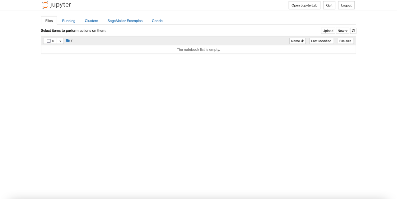
3. Open a browser and navigate to the PreSignedURL from the previous step.

The webpage should look like the following screenshot.

Conclusion

In this post, we demonstrated how to deploy the infrastructure components for a SageMaker notebook instance environment using AWS CloudFormation. We then illustrated how to use EventBridge to return the notebook instance state from the AWS Service Catalog API. Lastly, we showed how to use a Lambda function to return the presigned notebook instance URL for accessing the delivered resource. For more information, see the Amazon SageMaker Developer Guide. Thank you for reading!

About the Authors

Joe Keating is a Senior Customer Delivery Architect in Professional Services at Amazon Web Services. He works with AWS customers to design and implement a variety of solutions in the AWS Cloud. Joe enjoys cooking with a glass or two of wine and achieving mediocrity on the golf course.

Matt Hedges is a Cloud Application Architect at Amazon Web Services. He works closely with customers to align technology needs with business drivers to deliver their applications on AWS. With a focus on migrations and modernization, Matt works with enterprise customers around the world to pioneer changes that unlock the full potential of the cloud. Matt enjoys spending time with family, playing musical instruments, cooking, playing video games, fixing old cars, and learning new things.

Virginia Chu is a Senior DevSecOps Architect in Professional Services at Amazon Web Services. She works with enterprise-scale customers around the globe to design and implement a variety of solutions in the AWS Cloud.

Read More

In December 2020, AWS announced the general availability of Amazon SageMaker JumpStart, a capability of Amazon SageMaker that helps you quickly and easily get started with machine learning (ML). JumpStart provides one-click fine-tuning and deployment of a wide variety of pre-trained models across popular ML tasks, as well as a selection of end-to-end solutions that solve common business problems. These features remove the heavy lifting from each step of the ML process, making it easier to develop high-quality models and reducing time to deployment.

All JumpStart content was previously available only through Amazon SageMaker Studio, which provides a user-friendly graphical interface to interact with the feature. Recently, we also announced the launch of easy-to-use JumpStart APIs as an extension of the SageMaker Python SDK, allowing you to programmatically deploy and fine-tune a vast selection of JumpStart-supported pre-trained models on your own datasets. This launch unlocks the usage of JumpStart capabilities in your code workflows, MLOps pipelines, and anywhere else you are interacting with SageMaker via SDK.

This post is the second in a series on using JumpStart for specific tasks. In the first post, we showed how you can run image classification use cases on JumpStart. In this post, we provide a step-by-step walkthrough on how to fine-tune and deploy a text classification model, using trained models from TensorFlow Hub. We explore two ways of obtaining the same result: via JumpStart’s graphical interface on Studio, and programmatically through JumpStart APIs. While not used in this blog post, Amazon Comprehend is a natural language processing (NLP) service that uses machine learning (ML) to find insights and relationships like people, places, sentiments, and topics in text. In a fully-managed experience, customers can use Comprehend’s custom classification API to train a custom classification model to recognize the classes that are of interest and then use that model to classify documents into your own categories.

If you want to jump straight into the JumpStart API code we explain in this post, you can refer to the following sample Jupyter notebooks:

• Introduction to JumpStart – Text Classification
• Introduction to JumpStart – Sentence Pair Classification

JumpStart overview

JumpStart is a multi-faceted product that includes different capabilities to help get you quickly started with ML on SageMaker. At the time of writing, JumpStart enables you to do the following:

• Deploy pre-trained models for common ML tasks – JumpStart enables you to address common ML tasks with no development effort by providing easy deployment of models pre-trained on large, publicly available datasets. The ML research community has put a large amount of effort into making a majority of recently developed models publicly available for use. JumpStart hosts a collection of over 300 models, spanning the 15 most popular ML tasks such as object detection, text classification, and text generation, making it easy for beginners to use them. These models are drawn from popular model hubs such as TensorFlow, PyTorch, Hugging Face, and MXNet Hub.
• Fine-tune pre-trained models – JumpStart allows you to fine-tune pre-trained models with no need to write your own training algorithm. In ML, the ability to transfer the knowledge learned in one domain to another domain is called transfer learning. You can use transfer learning to produce accurate models on your smaller datasets, with much lower training costs than the ones involved in training the original model. JumpStart also includes popular training algorithms based on LightGBM, CatBoost, XGBoost, and Scikit-learn, which you can train from scratch for tabular regression and classification.
• Use pre-built solutions – JumpStart provides a set of 17 solutions for common ML use cases, such as demand forecasting and industrial and financial applications, which you can deploy with just a few clicks. Solutions are end-to-end ML applications that string together various AWS services to solve a particular business use case. They use AWS CloudFormation templates and reference architectures for quick deployment, which means they’re fully customizable.
• Refer to notebook examples for SageMaker algorithms – SageMaker provides a suite of built-in algorithms to help data scientists and ML practitioners get started with training and deploying ML models quickly. JumpStart provides sample notebooks that you can use to quickly use these algorithms.
• Review training videos and blogs – JumpStart also provides numerous blog posts and videos that teach you how to use different functionalities within SageMaker.

JumpStart accepts custom VPC settings and AWS Key Management Service (AWS KMS) encryption keys, so you can use the available models and solutions securely within your enterprise environment. You can pass your security settings to JumpStart within Studio or through the SageMaker Python SDK.

Transformer models and the importance of fine-tuning

The attention-based Transformer architecture has become the de-facto standard for the state-of-the-art natural language processing (NLP) models. In 2018, the famous BERT model was born from an adapted Transformer encoder, pre-trained on GBs of unlabeled English text from Wikipedia and other public resources. BERT was incredibly useful for creating contextualized text representations, which you could then use in many downstream tasks by fine-tuning the model. Since then, many variants of the BERT model have been developed by way of architecture, pre-training schema, or pre-training dataset changes.

Fine-tuning means to use a model that has been pre-trained on a given task and train it again, this time for a specific task that is different but related (and on your specific data). This practice is also typically referred to as transfer learning—literally meaning to transfer knowledge gained on one task to another. Typically, Transformer-based models are pre-trained on massive amounts of unlabeled data, and comparatively much smaller labeled datasets are then used for fine-tuning. Being able to leverage the large computational investments made to pre-train such models for downstream tasks (commonly made open-source) has been one of the most important factors in the growth of NLP as a field in previous years. However, as new models get larger and more complex, so does the development effort required to fine-tune and deploy them efficiently. In this post, we show you how to use JumpStart to fine-tune a BERT model with little to no development effort involved.

Text classification

Sentiment analysis is one of the many tasks under the umbrella of text classification. It consists of predicting what sentiment should be assigned to a specific passage of text, with varying degrees of granularity. Typical applications include social media monitoring, customer support management, and analyzing customer feedback.

The input is a directory containing a data.csv file. The first column is the label (an integer between 0 and the number of classes in the dataset), and the second column is the corresponding passage of text. This means that you could even use a dataset with more degrees of sentiment than the original—for example, very negative (0), negative (1), neutral (2), positive (3), very positive (4). The following is an example of a data.csv file corresponding to the SST2 (Stanford Sentiment Treebank) dataset, and shows values in its first two columns. Note that the file shouldn’t have any header.

The SST2^1,2 dataset is downloaded from TensorFlow. Apache 2.0 License. Dataset Homepage.

Sentence pair classification

Sentence pair classification consists of predicting a class for a pair of sentences, which forces the model to learn semantic dependencies between sentence pairs. Among these are typically textual entailment (does the first sentence come before the second originally?), paraphrasing (are both sentences just differently worded versions of one another?), and others.

The input is a directory containing a data.csv file. The first column in the file should have integer class labels between 0 and the number of classes. The second and third columns should contain the first and second sentence corresponding to that row. The following is an example of a data.csv file for the QNLI dataset, and shows values in its first three columns. Note that the file shouldn’t have any header.

The QNLI^3.4 dataset is downloaded from TensorFlow. Apache 2.0 License. Dataset Homepage. CC BY-SA 4.0 License.

Solution overview

The following sections provide a step-by-step demo to perform sentiment analysis with JumpStart, both via the Studio UI and via JumpStart APIs. The workflow for sentence pair classification is almost identical, and we describe the changes required for that task.

We walk through the following steps:

1. Access JumpStart through the Studio UI:
   1. Fine-tune the pre-trained model.
   2. Deploy the fine-tuned model.
2. Use JumpStart programmatically with the SageMaker Python SDK:
   1. Fine-tune the pre-trained model.
   2. Deploy the fine-tuned model.

Access JumpStart through the Studio UI

In this section, we demonstrate how to train and deploy JumpStart models through the Studio UI.

Fine-tune the pre-trained model

The following video shows you how to find a pre-trained text classification model on JumpStart and fine-tune it on the task of sentiment analysis. The model page contains valuable information about the model, how to use it, expected data format, and some fine-tuning details.

For demonstration purposes, we fine-tune the model using the dataset provided by default, which is the Stanford Sentiment Treebank v2 (SST2) dataset. Fine-tuning on your own dataset involves taking the correct formatting of data (as explained on the model page), uploading it to Amazon Simple Storage Service (Amazon S3), and specifying its location in the data source configuration.

We use the sane hyperparameter values set by default (number of epochs, learning rate, and batch size). We also use a GPU-backed ml.p3.2xlarge as our SageMaker training instance.

You can monitor your training job running directly on the Studio console, and are notified upon its completion.

For sentence pair classification, instead of searching for text classification models in the JumpStart search bar, search for sentence pair classification. For example, choose Bert Base Uncased from the resulting model selection. Apart from the dataset format, the rest of the workflow is identical between text classification and sentence pair classification.

Deploy the fine-tuned model

After training is complete, you can deploy the fine-tuned model from the same page that holds the training job details. To deploy our model, we pick a different instance type, ml.g4dn.xlarge. It still provides the GPU acceleration needed for low inference latency, but at a lower price point. After you configure the SageMaker hosting instance, choose Deploy. It may take 5–10 minutes until your persistent endpoint is up and running.

After a few minutes, your endpoint is operational and ready to respond to inference requests!

To accelerate your time to inference, JumpStart provides a sample notebook that shows you how to run inference on your freshly deployed endpoint. Choose Open Notebook under Use Endpoint from Studio.

Use JumpStart programmatically with the SageMaker SDK

In the preceding sections, we showed how you can use the JumpStart UI to fine-tune and deploy a model interactively, in a matter of a few clicks. However, you can also use JumpStart’s models and easy fine-tuning programmatically by using APIs that are integrated into the SageMaker SDK. We now go over a quick example of how you can replicate the preceding process. All the steps in this demo are available in the accompanying notebooks Introduction to JumpStart – Text Classification and Introduction to JumpStart – Sentence Pair Classification.

Fine-tune the pre-trained model

To fine-tune a selected model, we need to get that model’s URI, as well as that of the training script and the container image used for training. Thankfully, these three inputs depend solely on the model name, version (for a list of the available models, see JumpStart Available Model Table), and the type of instance you want to train on. This is demonstrated in the following code snippet:

from sagemaker import image_uris, model_uris, script_uris

model_id, model_version = "tensorflow-tc-bert-en-uncased-L-12-H-768-A-12-2", "1.0.0"
training_instance_type = "ml.p3.2xlarge"

# Retrieve the docker image
train_image_uri = image_uris.retrieve(
    region=None,
    framework=None,
    model_id=model_id,
    model_version=model_version,
    image_scope="training",
    instance_type=training_instance_type,
)
# Retrieve the training script

train_source_uri = script_uris.retrieve(model_id=model_id, model_version=model_version, script_scope="training")

# Retrieve the pre-trained model tarball to further fine-tune

train_model_uri = model_uris.retrieve(model_id=model_id, model_version=model_version, model_scope="training")

We retrieve the model_id corresponding to the same model we used previously (dimensions are characteristic to the base version of BERT). The tc in the identifier corresponds to text classification.

For sentence pair classification, we can set model_id to huggingface-spc-bert-base-uncased. The spc in the identifier corresponds to sentence pair classification.

You can now fine-tune this JumpStart model on your own custom dataset using the SageMaker SDK. We use a dataset that is publicly hosted on Amazon S3, conveniently focused on sentiment analysis. The dataset should be structured for fine-tuning as explained in the previous section. See the following example code:

# URI of your training dataset
training_dataset_s3_path = "s3://jumpstart-cache-prod-us-west-2/training-datasets/tc/data.csv"
training_job_name = name_from_base(f"jumpstart-example-{model_id}-transfer-learning")

# Create SageMaker Estimator instance
tc_estimator = Estimator(
    role=aws_role,
    image_uri=train_image_uri,
    source_dir=train_source_uri,
    model_uri=train_model_uri,
    entry_point="transfer_learning.py",
    instance_count=1,
    instance_type=training_instance_type,
    max_run=360000,
    hyperparameters=hyperparameters,
    output_path=s3_output_location,
)

# Launch a SageMaker Training job by passing s3 path of the training data
tc_estimator.fit({"training": training_dataset_s3_path}, logs=True)

We obtain the same default hyperparameters for our selected model as the ones we saw in the previous section, using sagemaker.hyperparameters.retrieve_default(). We then instantiate a SageMaker estimator, and call the .fit method to start fine-tuning our model, passing it the Amazon S3 URI for our training data. As you can see, the entry_point script provided is named transfer_learning.py (the same for other tasks and models), and the input data channel passed to .fit must be named training.

Deploy the fine-tuned model

When training is complete, you can deploy your fine-tuned model. To do so, all we need to obtain is the inference script URI (the code that determines how the model is used for inference once deployed) and the inference container image URI, which includes an appropriate model server to host the model we chose. See the following code:

# Retrieve the inference docker container uri
deploy_image_uri = image_uris.retrieve(
    region=None,
    framework=None,
    image_scope="inference",
    model_id=model_id,
    model_version=model_version,
    instance_type=inference_instance_type,
)
# Retrieve the inference script uri
deploy_source_uri = script_uris.retrieve(
    model_id=model_id, model_version=model_version, script_scope="inference"
)

endpoint_name = name_from_base(f"jumpstart-example-FT-{model_id}-")

# Use the estimator from the previous step to deploy to a SageMaker endpoint
finetuned_predictor = tc_estimator.deploy(
    initial_instance_count=1,
    instance_type=inference_instance_type,
    entry_point="inference.py",
    image_uri=deploy_image_uri,
    source_dir=deploy_source_uri,
    endpoint_name=endpoint_name,
)

After a few minutes, our model is deployed and we can get predictions from it in real time!

Next, we invoke the endpoint to predict the sentiment of the example text. We use the query_endpoint and parse_response helper functions, which are defined in the accompanying notebook:

text = "simply stupid , irrelevant and deeply , truly , bottomlessly cynical "
query_response = query_endpoint(text.encode("utf-8"))
probabilities, labels, predicted_label = parse_response(query_response)

Conclusion

JumpStart is a capability in SageMaker that allows you to quickly get started with ML. JumpStart uses open-source pre-trained models to solve common ML problems like image classification, object detection, text classification, sentence pair classification, and question answering.

In this post, we showed you how to fine-tune and deploy a pre-trained text classification model for sentiment analysis. We also mentioned the changes required to adapt the demo for sentence pair classification. With JumpStart, you can easily do this process with no need to code. Try out the solution on your own and let us know how it goes in the comments. To learn more about JumpStart, check out the AWS re:Invent 2020 video Get started with ML in minutes with Amazon SageMaker JumpStart.

References

1. Socher et al., 2013
2. Wang et al., 2018a
3. Rajpurkar et al., 2016
4. Wang et al., 2018a

About the Authors

João Moura is an AI/ML Specialist Solutions Architect at Amazon Web Services. He is mostly focused on NLP use cases and helping customers optimize Deep Learning model training and deployment. He is also an active proponent of low-code ML solutions and ML-specialized hardware.

Dr. Vivek Madan is an Applied Scientist with Amazon SageMaker JumpStart team. He got his PhD from University of Illinois at Urbana-Champaign and was a Post Doctoral Researcher at Georgia Tech. He is an active researcher in machine learning and algorithm design and has published papers in EMNLP, ICLR, COLT, FOCS and SODA conferences.

Dr. Ashish Khetan is a Senior Applied Scientist with Amazon SageMaker JumpStart and Amazon SageMaker built-in algorithms and helps develop machine learning algorithms. He is an active researcher in machine learning and statistical inference and has published many papers in NeurIPS, ICML, ICLR, JMLR, ACL, and EMNLP conferences.

Read More

Amazon Lookout for Metrics is an AWS service that uses machine learning (ML) to automatically monitor the metrics that are most important to businesses with greater speed and accuracy. The service also makes it easier to diagnose the root cause of anomalies, such as unexpected dips in revenue, high rates of abandoned shopping carts, spikes in payment transaction failures, increases in new user sign-ups, and many more. Lookout for Metrics goes beyond simple anomaly detection. It allows developers to set up autonomous monitoring for important metrics to detect anomalies and identify their root cause in a matter of a few clicks to detect anomalies in its metrics—all with no ML experience required.

Amazon Athena is an interactive query service that makes it easy to analyze data in Amazon Simple Storage Service (Amazon S3) using standard SQL. Simply point to your data in Amazon S3, define the schema, and start querying using standard SQL. Most results are delivered within seconds. With Athena, there’s no need for complex ETL jobs to prepare your data for analysis. This makes it easy for anyone with SQL skills to quickly analyze large-scale datasets.

With today’s launch, Lookout for Metrics can now seamlessly connect to your data in Athena to set up highly accurate anomaly detectors. This lets you quickly deploy state-of-the-art anomaly detection via ML with Lookout for Metrics against any datasets that are available in Athena.

Athena connectivity extends the capabilities of Lookout for Metrics by bringing the following benefits:

• It extends the capabilities of Lookout for Metrics in terms of filetype support. Prior to this, Lookout for Metrics supported CSV and JSONLines formatted files, but with Athena this has been expanded to Parquet, Avro, Plaintext, and more. If you can parse it via Athena, then it’s now possible to import and leverage with Lookout for Metrics.
• It also introduces support for data with federated queries. Prior to this launch, if your data was stored in multiple databases or sources, you would need to define a complete complex ETL process as well as manage its performance characteristics before you could export all of the data into a CSV or JSONLines file and input it into Lookout for Metrics for Anomaly Detection. With federated queries from Athena, you define the disparate sources as well as how the join should be performed and when the data has been processed and can be queried by Athena, it’s immediately ready for Lookout for Metrics. This enables you to hand over the burden for data transformation, aggregation, and delivery location to Athena and just focus on the identified anomalies from Lookout for Metrics.

Solution overview

In this post, we demonstrate how to integrate an Athena table and detect anomalies in the revenue metrics. We also track how order rate and inventory metrics are impacted. The source data lies in Amazon S3 and we’ve configured Athena tables to be able to query the data in it. An AWS Lambda is responsible for updating the partitions within Athena, which are used by Lookout for Metrics to detect anomalies. This solution enables you to use an Athena data source for Lookout for Metrics.

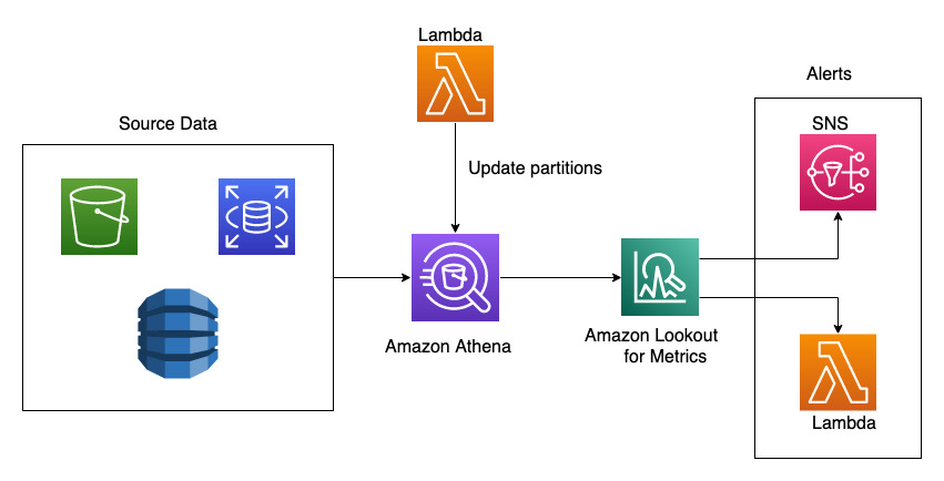
You could use the provided AWS CloudFormation stack to set up resources for the walkthrough. It contains resources to continuously generate live data and makes them query-able in Athena.

• Launch the stack from the following link and select next on the Create Stack page.
  
• On the Specify stack details page, add the values from above, give it a Stack name (for example, L4MAthenaDetector), and select Next.
• On the Configure stack options page, leave everything as-is and select Next.

Set up a new detector with Athena as the data source

Step 1

Log in to the AWS Console to get started with creating an Anomaly Detector with Lookout for Metrics. The first step is to select the “Create detector” button.

Step 2

Fill out the mandatory detector fields like name. Select the detection interval for the detector, which is determined by the frequency at which you want Lookout for Metrics to query your data and monitor them for anomalies. Encryption information is not mandatory. Encryption information allows Lookout for Metrics to encrypt your data using your AWS Key Management Service (KMS) key. In this example, we’ll skip adding an encryption key, Lookout for Metrics would use default encryption to encrypt your data if no encryption information is provided, and proceed by selecting the “Create” button.

Step 3

Upon creation of the anomaly detector, you’ll see confirmation in a banner at the top. You can proceed by selecting “Add a dataset” through either the banner or the button under “Add a dataset”.

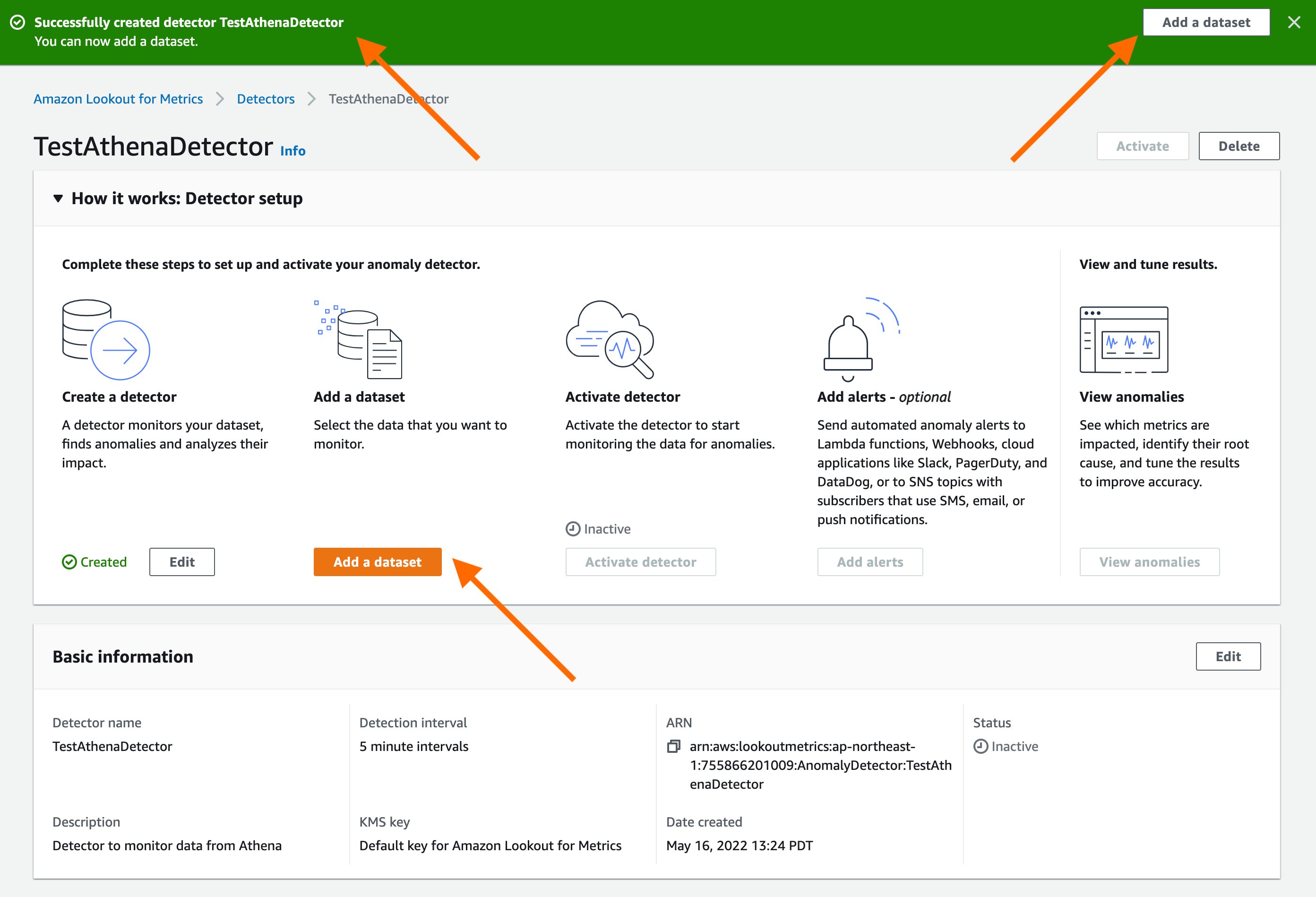
Fill out the basic information for the data source. Timezone is an optional field. Select the dropdown to select a data source.

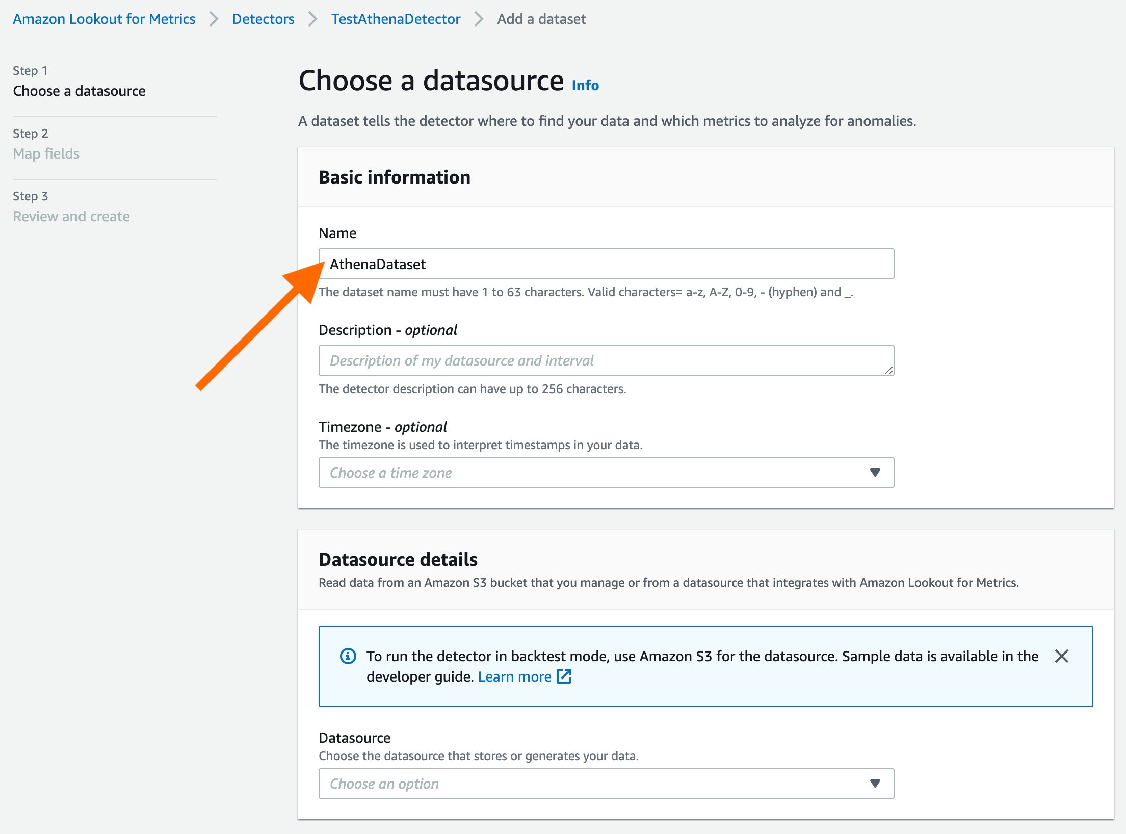
Lookout for Metrics supports multiple data sources as a convenience for customers. For this example, we’ll select Athena.

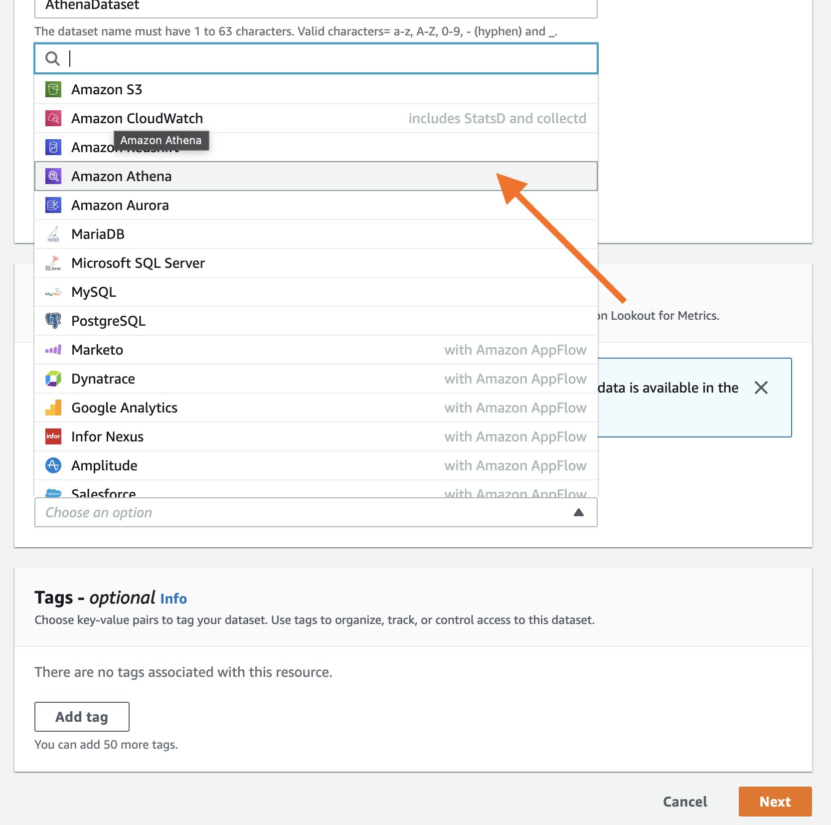
Once Athena is selected as the data source, you’ll have the option of selecting Backtest or Continuous mode for the detector. For this example, we’ll proceed by using the Continuous mode. Proceed by adding details for the Athena table that you want to monitor for anomalies.

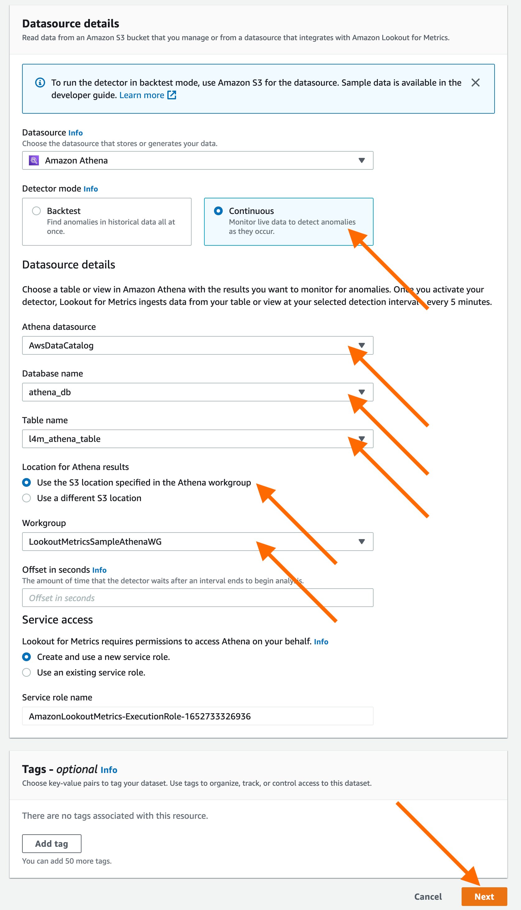
You can allow the service to create a Service role or you could use an existing AWS Identity and Access Management (IAM) role in your account for federated queries. Note that Lookout for Metrics doesn’t support automated creation of IAM roles for federated queries. Therefore, you would have to create a new IAM role to allow Athena to perform the following actions on your data,

• CreatePreparedStatement
• GetPreparedStatement
• GetQueryResultsStream
• DeletePreparedStatement
• GetDatabase
• GetQueryResults
• GetWorkGroup
• GetTableMetadata
• StartQueryExecution
• GetQueryExecution

The IAM role created by the service looks like the following:

{
  "Version": "2012-10-17",
  "Statement": [
    {
      "Action": [
        "glue:GetTable",
        "glue:GetDatabase",
        "glue:GetPartitions"
      ],
      "Resource": [
        "arn:aws:glue:us-east-1:111122223333:catalog",
        "arn:aws:glue:us-east-1:111122223333:database/sample_db",
        "arn:aws:glue:us-east-1:111122223333:table/sample_db/*"
      ],
      "Effect": "Allow"
    },
    {
      "Action": [
        "athena:CreatePreparedStatement",
        "athena:GetPreparedStatement",
        "athena:GetQueryResultsStream",
        "athena:DeletePreparedStatement",
        "athena:GetDatabase",
        "athena:GetQueryResults",
        "athena:GetWorkGroup",
        "athena:GetTableMetadata",
        "athena:StartQueryExecution",
        "athena:GetQueryExecution"
      ],
      "Resource": [
          "arn:aws:athena:us-east-1:111122223333:datacatalog/AWSDataCatalog",
          "arn:aws:athena:us-east-1:111122223333:workgroup/sampleWorkgroup"
      ],
      "Effect": "Allow"
    },
    {
      "Action": [
        "s3:GetObject",
        "s3:ListBucket",
        "s3:PutObject",
        "s3:GetBucketLocation",
        "s3:ListBucketMultipartUploads",
        "s3:ListMultipartUploadParts",
        "s3:AbortMultipartUpload"
      ],
      "Resource": [
        "arn:aws:s3:::sample-data-bucket",
        "arn:aws:s3:::sample-results-bucket",
        "arn:aws:s3:::sample-data-bucket/*",
        "arn:aws:s3:::sample-results-bucket/*"
      ],
      "Effect": "Allow"
    },
    {
      "Effect": "Allow",
      "Action": [
        "kms:GenerateDataKey",
        "kms:Decrypt"
      ],
      "Resource": [
        "*"
      ],
      "Condition": {
        "ForAllValues:StringEquals": {
          "kms:ViaService": "s3.us-east-1.amazonaws.com",
          "kms:CallerAccount": [
            "111122223333"
          ]
        }
      }
    }
  ]
}

Step 4

Now we’ll define relevant metrics for the detector. Lookout for Metrics will populate the drop-downs with the columns present in the supplied Athena table. You can select up to five metrics and five dimensions. Lookout for Metrics requires the data in your table to be partitioned as timestamps for the timestamp column. You will also have an option to estimate the cost for this detector by adding the number of values across your dimensions.

Once you have selected all of the metrics, proceed by selecting the “Next” button. Review the details and select the “Save dataset” button to save the dataset.

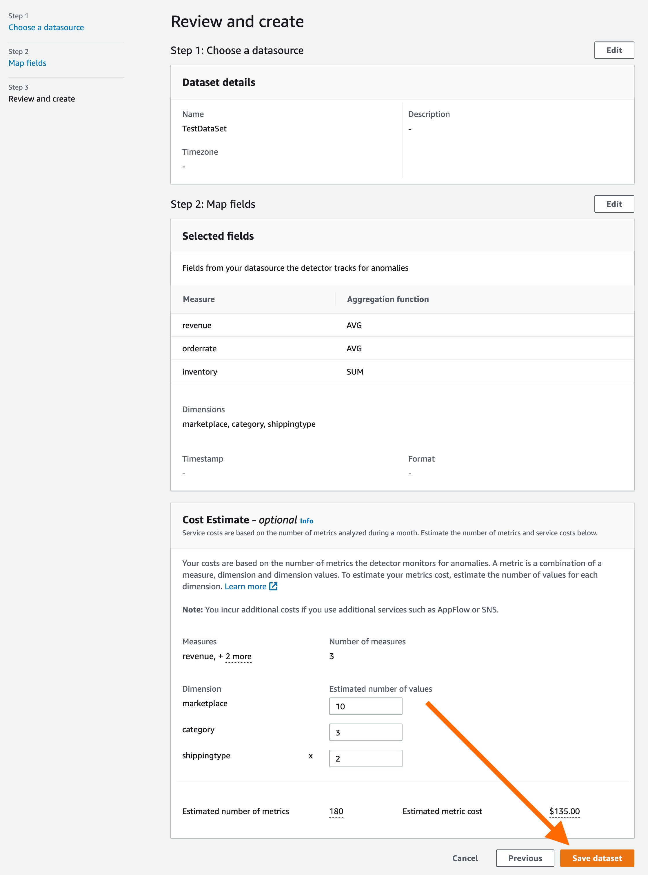
Step 5

Once the dataset is created, we’ll activate the detector by either selecting the “Activate” button at the top or the “Activate Detector” button under the “How it works” section.

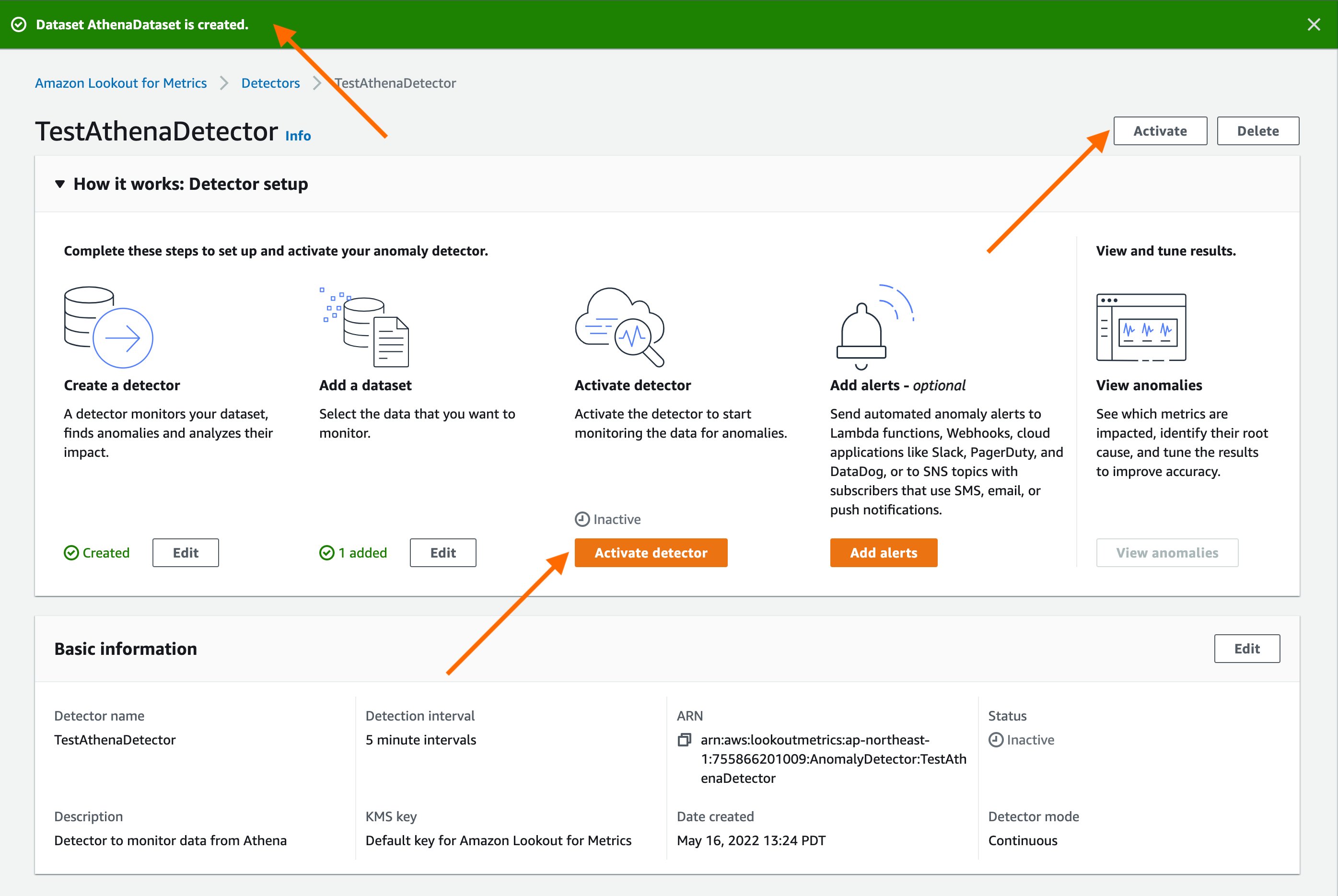
You’ll be prompted to confirm if you want to activate the detector for continuous detection. Select “Activate” to confirm.

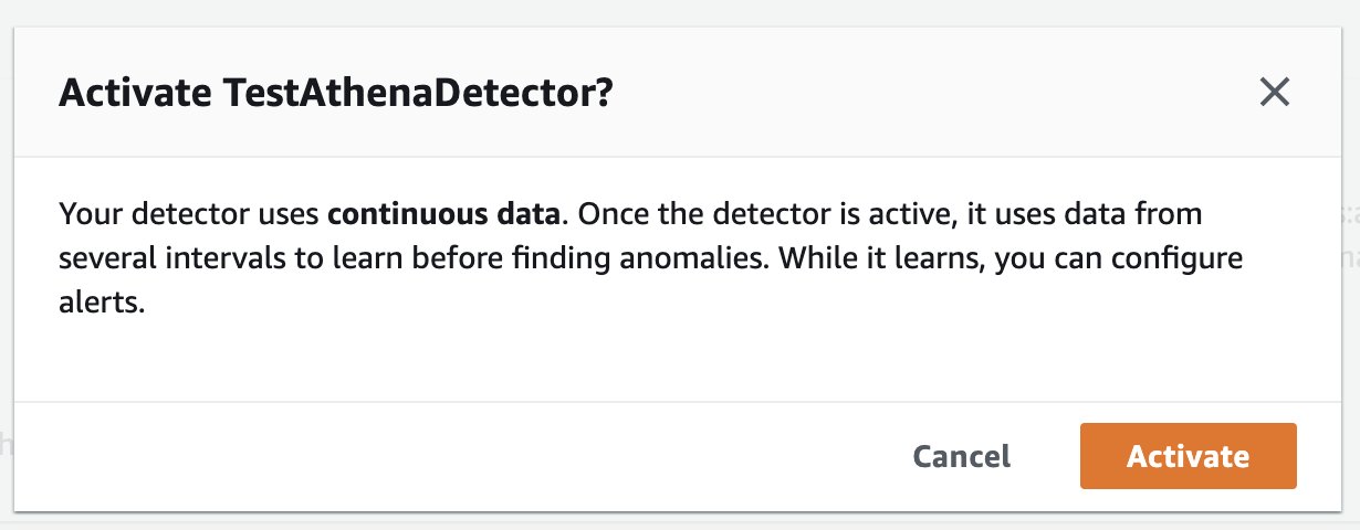
You’ll see a confirmation informing that the detector is activating.

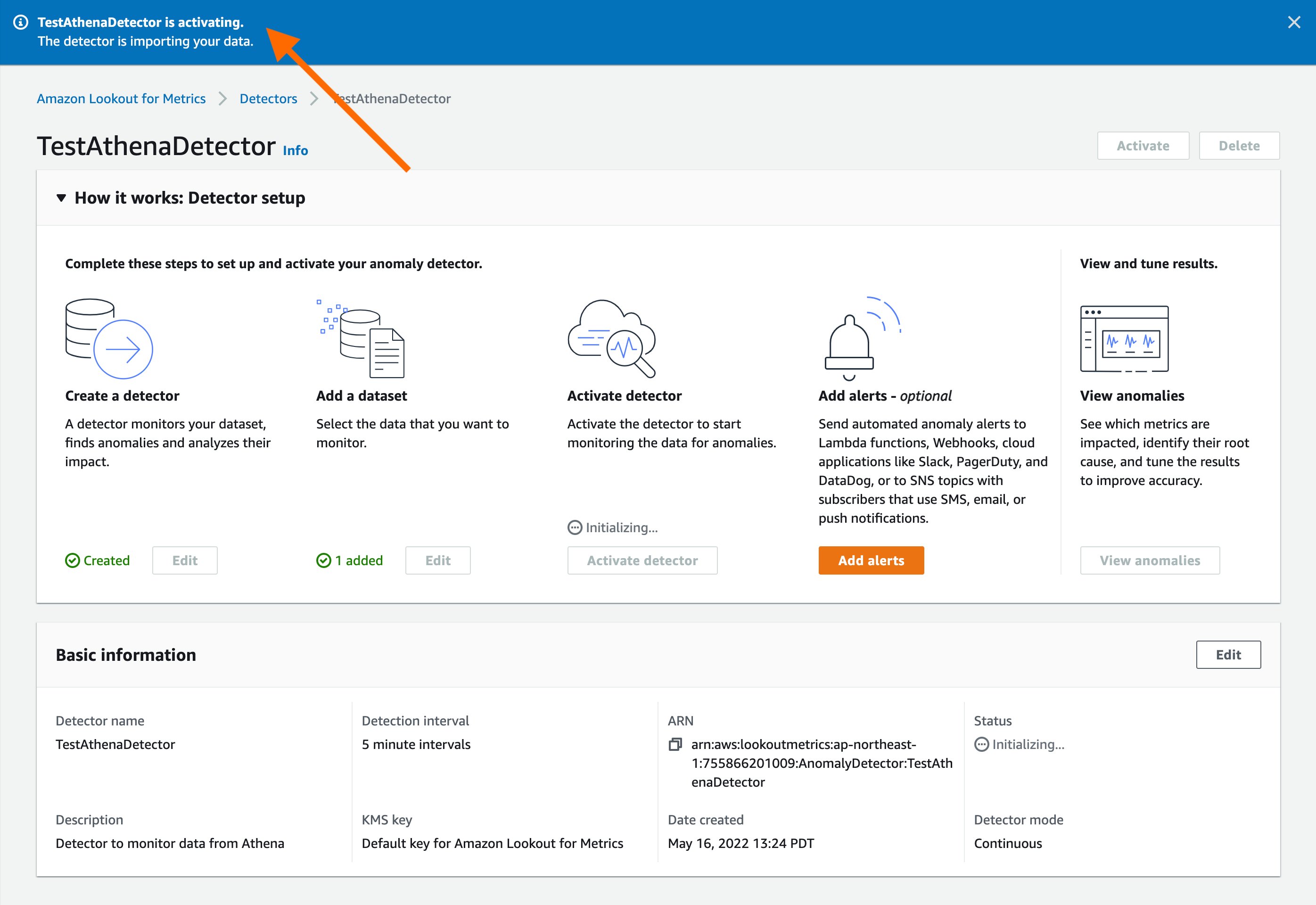
Step 6

Once the Anomaly Detector is Active, you can use the “Detector log” tab on the Detector details page to review detection executions that have been performed by the service.

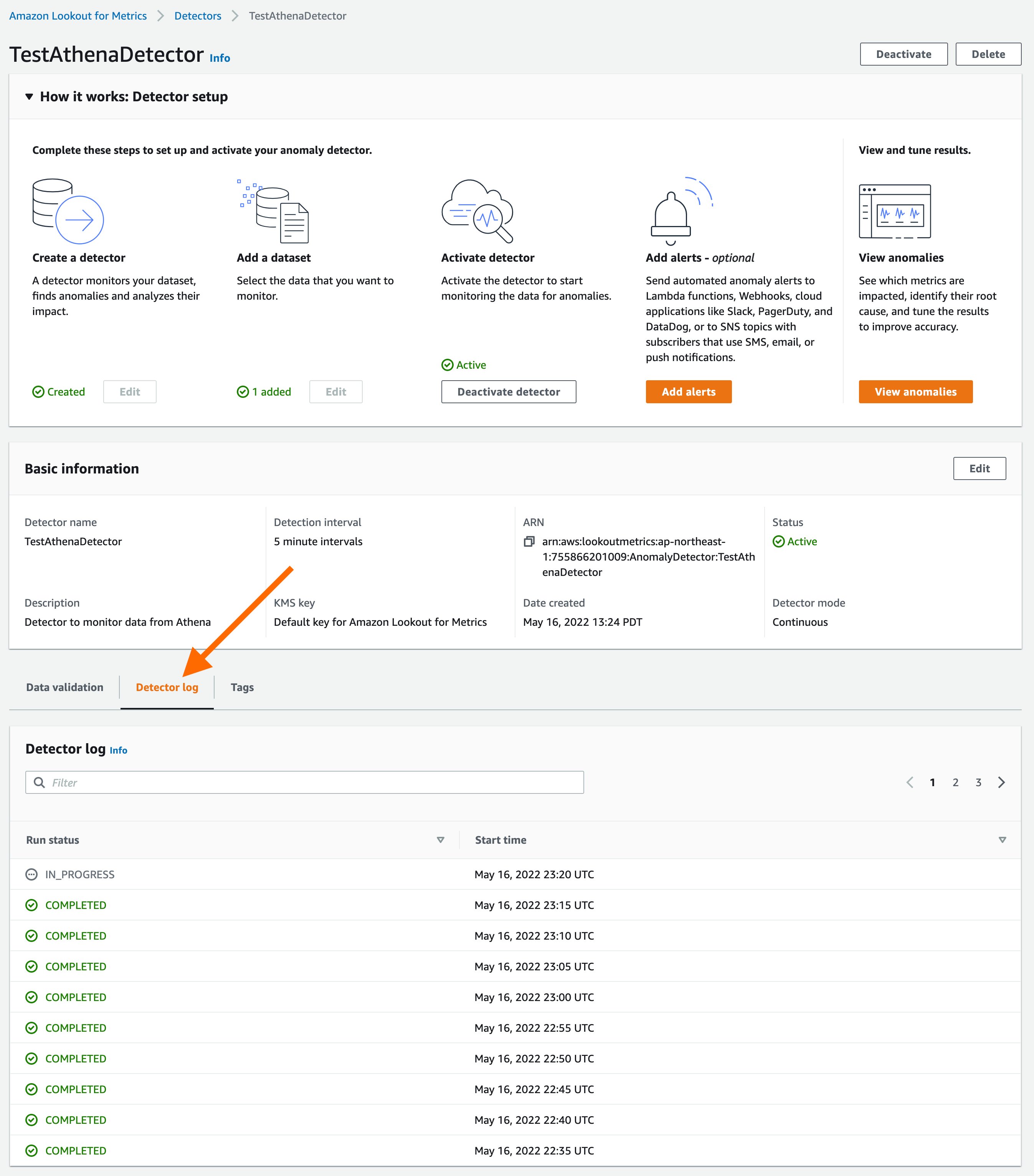
Step 7

You can select the “View anomalies” button from the detector details page to manually inspect anomalies that may have been detected by the service.

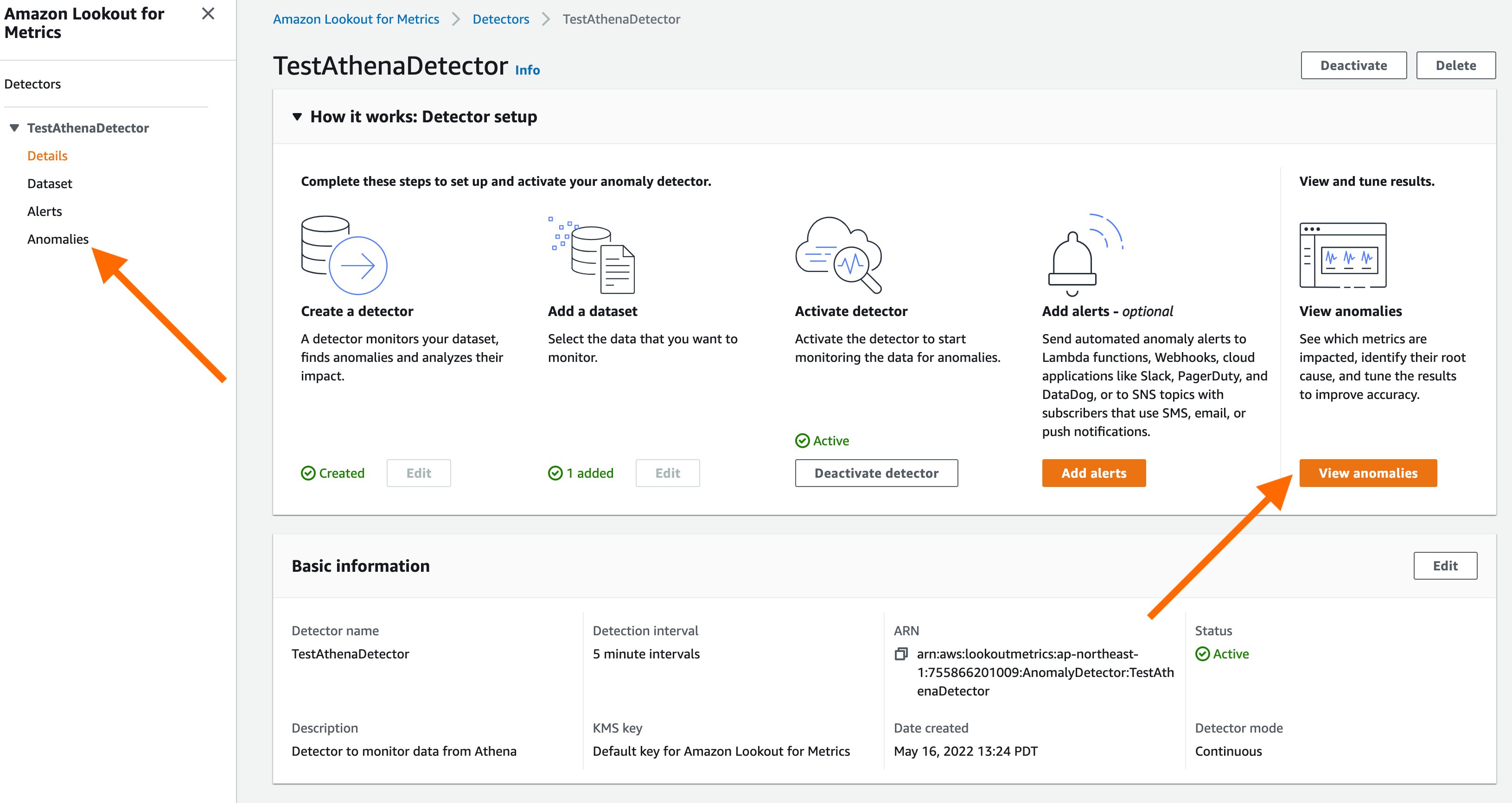
Step 8

On the Anomalies review page, you can adjust the severity score threshold on the threshold dial to filter anomalies above a selected score.

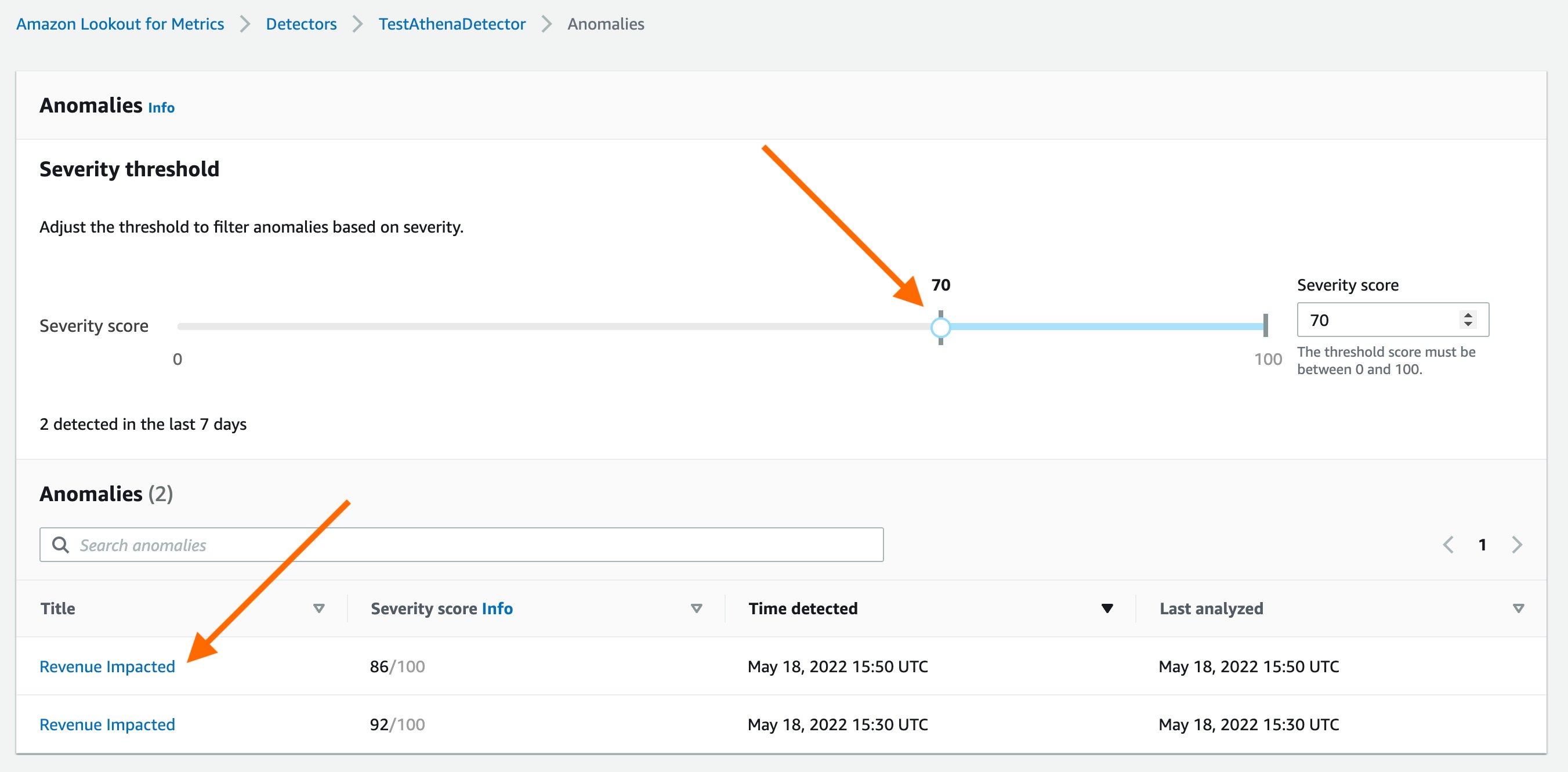
Review and analyze the results

When detecting an anomaly, Lookout for Metrics helps you focus on what matters most by assigning a severity score to aid prioritization. To help you find the root cause, it intelligently groups anomalies that may be related to the same incident, and then summarizes the different sources of impact.

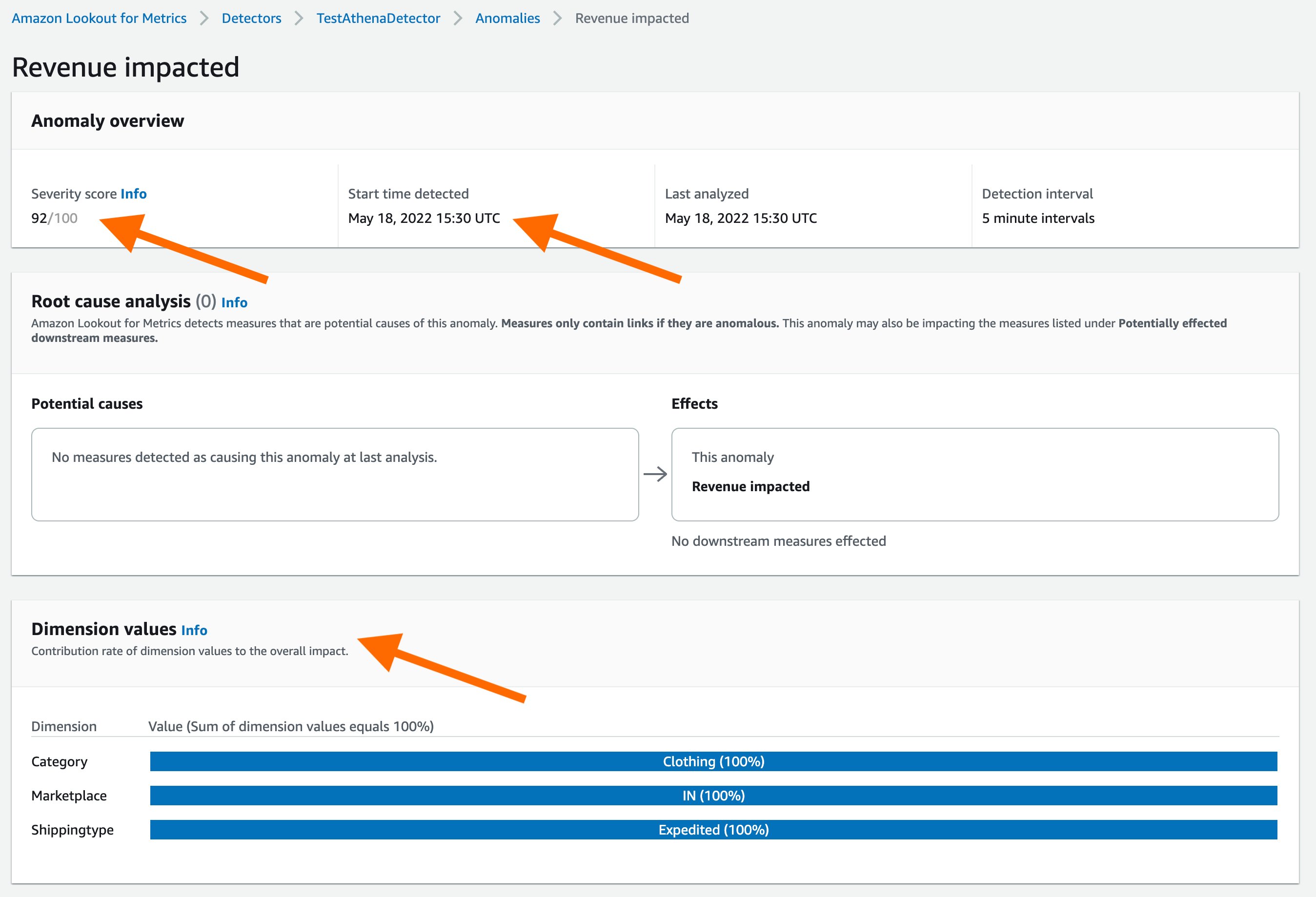
Lookout for Metrics also lets you provide real-time feedback on the relevance of detected anomalies, thereby enabling a powerful human-in-the-loop mechanism. This information is fed back to the anomaly detection model to improve its accuracy in near-real time.

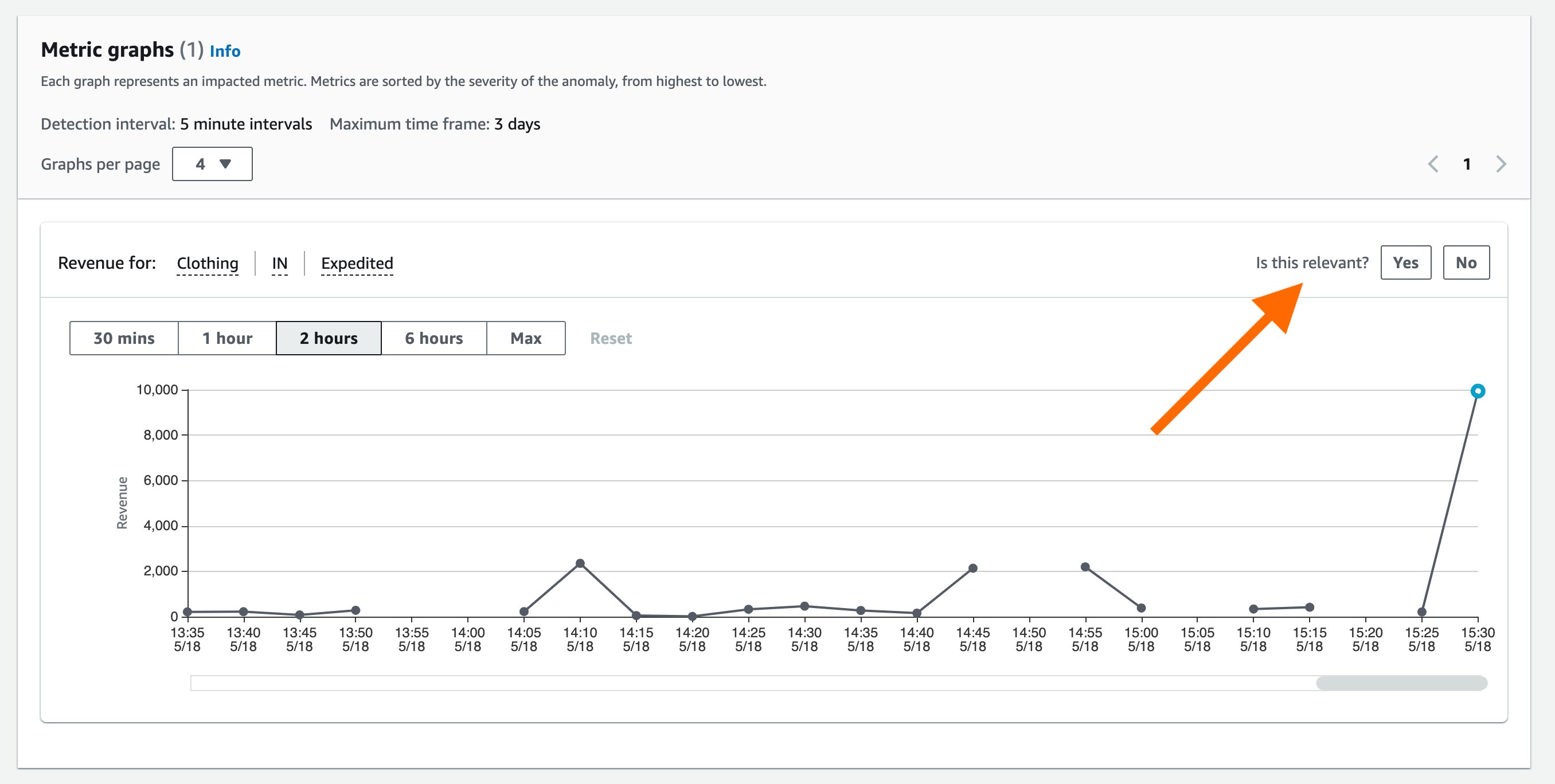
Clean up

To avoid incurring additional charges for the resource set up for the demo, you can delete the created detector under Lookout for Metrics and the stack created via CloudFormation.

Conclusion

You can seamlessly connect to your data in Athena to Lookout for Metrics to set up highly accurate anomaly detector across metrics and dimensions within your Athena tables. To get started with this capability, see Using Amazon Athena with Lookout for Metrics. You can use this capability in all Regions where Lookout for Metrics is publicly available. For more information about Region availability, see AWS Regional Services.

About the Authors

Devesh Ratho is a Software Development Engineer in the Lookout for Metrics team. His interests lie in building scalable distributed systems. In his spare time, he enjoys sim racing.

Chris King is a Senior Solutions Architect in Applied AI with AWS. He has a special interest in launching AI services and helped grow and build Amazon Personalize and Amazon Forecast before focusing on Amazon Lookout for Metrics. In his spare time he enjoys cooking, reading, boxing, and building models to predict the outcome of combat sports.

Read More