Conversational interfaces like chatbots have become an important channel for brands to communicate with their customers, partners, and employees. They offer faster service, 24/7 availability, and lower service costs. By analyzing your bot’s customer conversations, you can discover challenges in user experience, trending topics, and missed utterances. These additional insights can help you identify how to improve your bot and user engagement continuously. Whether you’re a product owner looking for user engagement insights or a conversation designer wanting to review missed utterances, a conversational analytics dashboard plays a vital role in serving these needs.
In this post, we build a real-time conversational analytics solution using the conversational logs from Amazon Lex. Amazon Lex is a service for building conversational interfaces into any application using voice and text. We use Amazon QuickSight to create a dashboard to visualize business KPIs, identify trends, and provide training data for bots to learn from their past failures. Some of the metrics we cover in this post include:
- Daily summary statistics
- User adoption
- Intent and utterance metrics
- Conversation review
- Sentiment analysis
Solution architecture
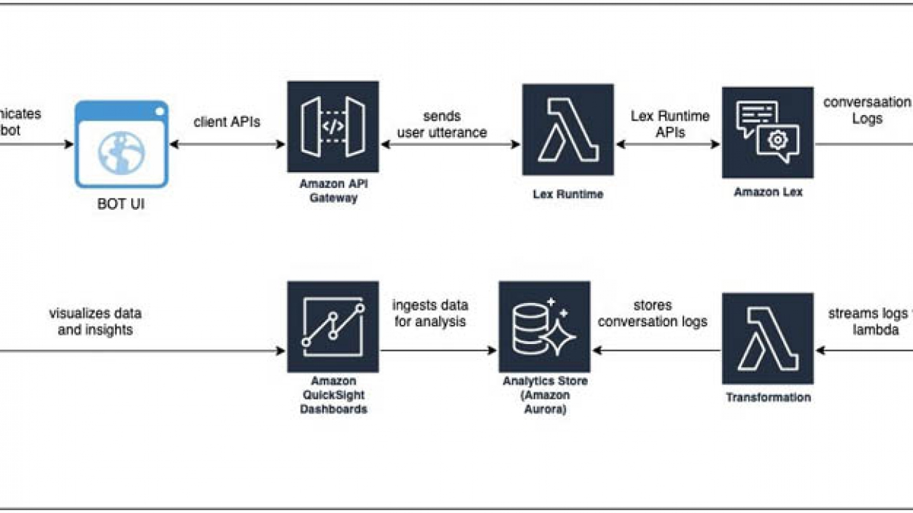
The following diagram illustrates the architecture of our solution.

The architecture comprises streaming the conversation logs from Amazon CloudWatch to Amazon Kinesis Data Streams and having a stream consumer (an AWS Lambda function) transforming the data to be written into an Amazon Aurora database that serves as the analytics store.
Depending on your project’s scale and your organizational needs and preferences, you may want to look into a data warehousing solution like Amazon Redshift or use Amazon Athena and Amazon Simple Storage Service (Amazon S3). For more information, see Building a business intelligence dashboard for your Amazon Lex bots.
We use the Aurora connector in QuickSight to pull in the data, create datasets and analysis, and publish a conversation analytics dashboard. QuickSight lets you easily create and publish interactive dashboards. You can choose from an extensive library of visualizations, charts, and tables, and add interactive features such as drill-downs and filters.
Solution overview
For this post, we created an Amazon Lex bot using the sample OrderFlowers blueprint. The default sample only comes with one intent: OrderFlowers. To make the analytics more interesting, we added custom intents like BusinessHoursIntent, OffersIntent, and MyFallbackIntent. For the export of this bot, download OrderFlowers.zip. You can import this file into your Amazon Lex console or use your own Amazon Lex bot.
To implement the solution, we need to complete the following tasks:
- Enable the conversation logs feature for your Amazon Lex bot.
- Create a Kinesis data stream and make it a subscriber to the CloudWatch log group created on the AWS CloudFormation
- Create an Aurora database to store the conversation log data.
- Create a Lambda function and subscribe it to listen to the data stream. The Lambda function extracts the data from the stream and writes it to the Aurora database.
- Set up QuickSight to consume data from the Aurora database.
- Create datasets and analysis, and publish the dashboard in QuickSight.
Deploying the CloudFormation template
The CloudFormation template deploys the following resources:
- An AWS Identity and Access Management (IAM) role to allow Amazon Lex to stream to CloudWatch Logs
- A CloudWatch log group
- A CloudWatch subscription filter
- A Kinesis data stream and its associated IAM role
- A Kinesis data stream consumer
- A Lambda function for object construction and its associated IAM role
- A serverless Aurora RDS cluster and its associated security group
- A security group for QuickSight access to Amazon Relational Database Service (Amazon RDS)
- An AWS Secrets Manager secret with Amazon RDS information
- A fresh VPC for the Aurora cluster
- Two subnets in the generated VPC
- A DB Subnet Group comprised of the two subnets
Complete the following steps:
- Deploy the template by choosing Launch Stack:
![]()
- Give your stack a unique name.
- Customize AWS CloudFormation deployment as needed.
- Deploy the template. This deployment should take approximately 5 minutes to complete
- Navigate to the Outputs tab of the CloudFormation stack and take note of the following values to use later:
SecretARNQuickSightSecurityGroupIDRDSEndpointRDSPort
Enabling the conversation logs option in your Amazon Lex bot
Conversation logs are generated when communicating with a Lex bot on an associated alias. Make sure that the AWS CloudFormation deployment is complete before attempting this step.
- On the Amazon Lex console, open your bot page and make sure the bot has been built and published.
- On the Settings tab, choose Conversation Logs.
- Publish an alias if you haven’t done so already by choosing the one you want and choosing the Settings
You’re prompted to select the log type, the CloudWatch log group, and IAM role on the next page.
- For Log Type, select Text logs.
- For Log Group, choose [STACK-NAME]
-LexAnalyticsLogGroup-[RANDOM-STRING]. - For IAM Role, choose [STACK-NAME]
-LexAnalyticsToCWLRole-[RANDOM-STRING].
You now create the FlowersLogs table in Amazon RDS.
- On the Amazon RDS console, navigate to the cluster created by the CloudFormation stack ([STACK-NAME]
-orderflowersrds-[RANDOM-STRING]). - Choose Query Editor.
- Select your RDS cluster.
- Choose Connect with a Secrets Manager ARN.
- Enter the
SecretARNfrom the Outputs tab of the CloudFormation stack. - Connect to the database and run the following query to create the table:
CREATE TABLE LexAnalyticsDB.FlowersLogs ( `id` mediumint(9) NOT NULL AUTO_INCREMENT, `botName` varchar(50) DEFAULT NULL, `botAlias` varchar(50) DEFAULT NULL, `botVersion` int(11) DEFAULT NULL, `inputTranscript` varchar(255) DEFAULT NULL, `botResponse` varchar(255) DEFAULT NULL, `intent` varchar(100) DEFAULT NULL, `slots` varchar(255) DEFAULT NULL, `missedUtterance` BOOLEAN DEFAULT NULL, `inputDialog` varchar(50) DEFAULT NULL, `requestId` varchar(255) DEFAULT NULL, `userId` varchar(100) DEFAULT NULL, `sessionId` varchar(255) DEFAULT NULL, `tmstmp` timestamp(2) NULL DEFAULT NULL, `sentiment` varchar(50) DEFAULT NULL, `topic` varchar(50) DEFAULT NULL, PRIMARY KEY (`id`) ) ENGINE=InnoDB AUTO_INCREMENT=2865933 DEFAULT CHARSET=latin1If you don’t have a client generating data on the Amazon Lex alias, you can generate test data using the aws-lex-web-ui deployment.
- Navigate to the aws-lex-web-ui GitHub repo.
- In the Getting Started section, choose Launch Stack for the Region you want to build in.
- For BotName, enter the name of your bot.
- For BotAlias, enter the alias of your bot.
- Keep the other settings at their default; they should be sufficient in generating sample data.
- Choose Create stack.
- When the stack is built, on the Outputs page, choose the link for WebAppUrl.
You can now use this page to generate traffic for your bot.
Configuring QuickSight access
For this post, we assume that you’re starting from scratch and haven’t signed up for QuickSight.
Create a VPC Connection in Amazon QuickSight
- On the QuickSight console, choose Sign up for QuickSight.

- Keep the default settings, and make sure that you deploy in the same region where you deployed your CloudFormation stack.
- On the Settings page, on the Manage VPC connections tab, choose Add VPC connection.

- Enter a connection name.
- Choose the same VPC you deployed your RDS instance into.
- Choose any subnet in the VPC.
- For Security Group ID, enter the
QuickSightSecurityGroupIDvalue from the Outputs tab of the CloudFormation stack. - Choose Create.
Create a Dataset in QuickSight
- Go to the Resources tab of your CloudFormation stack.
- Navigate to the LexAnalyticsSecret resource and choose the blue link to the resource.
- Choose Retrieve secret value.
- Copy the username and password.
- On the QuickSight console, choose Manage Data.
- Choose New Data Set.
- For Data source, choose Aurora.
- Enter a name for your data source.
- For Connection type, select the connection you created in the previous section.
- For Database connector, choose MySQL.
- For the server and port, use the
RDSEndpointandRDSPortfields from the CloudFormation stack Outputs. - For Database name, enter
LexAnalyticsDB. - Enter the username and password for the RDS instance earlier.
- Choose Create data source.
- Select the FlowersLogs
- Import to SPICE.
Configuring QuickSight visuals
You have an assortment of pivots to base the analytical dashboard on, depending on the use case you’re targeting: summary view, trend analysis, user level, intent level, utterance level, conversation review, and sentiment analysis.
A summary view can help you compare and contrast the number of users, sessions, and utterances between the current day and the previous day, or the current hour and the previous hour.

A trend analysis of sessions, users, and utterances can help you spot anomalies and cyclical patterns.

User-level metrics measure which users are adopting the chatbots more regularly versus users who are not. You can use this data in conjunction with persona data to segment users to create personalized experiences.

Intent-level metrics help identify the top N intents, which improves staffing decisions at the contact centers serving phone and chat channels. When deciding to prune a bot’s intent structure, you can use these metrics to remove the bottom N intents that don’t serve significant traffic.

Utterance-level metrics help you identify missed utterances and group them by phrases. You can either add the utterances with high counts to the existing intents or create new intents if those utterances don’t already fit into the existing intents.

Conversation review helps you look at the entire conversation between the user and the bot.

Sentiment analysis helps you learn your users’ overall sentiment concerning their experience with the bot. Reviewing conversations that received negative sentiment helps you identify the root cause.


Conclusion
Whether you’re a product owner, conversation designer, developer, or data scientist, conversational analytics are pivotal to understanding user adoption and teaching your bot to learn from its past mistakes. This post covered how to use conversation logs and QuickSight to capture useful insights from user conversations and visualize them. Get started with Amazon Lex and start building your a customized analytics dashboard for your conversation logs.
About the Authors
 Shanthan Kesharaju is a Senior Architect who helps our customers with AI/ML strategy and architecture. Shanthan has an MBA in Marketing from Duke University and an MS in Management Information Systems from Oklahoma State University.
 Blake DeLee is a Rochester, NY-based conversational AI consultant with AWS Professional Services. He has spent five years in the field of conversational AI and voice, and has experience bringing innovative solutions to dozens of Fortune 500 businesses. Blake draws on a wide-ranging career in different fields to build exceptional chatbot and voice solutions.


 Ben Snively is an AWS Public Sector Specialist Solutions Architect. He works with government, non-profit, and education customers on big data/analytical and AI/ML projects, helping them build solutions using AWS.
 Sam Palani is an AI/ML Specialist Solutions Architect at AWS. He works with public sector customers to help them architect and implement machine learning solutions at scale. When not helping customers, he enjoys long hikes, unwinding with a good book, listening to his classical vinyl collection and hacking projects with Raspberry Pi.

 BK Chaurasiya is a Principal Product Manager at Amazon Web Services R&D and Innovation team. He provides technical guidance, design advice, and thought leadership to some of the largest and successful AWS customers and partners. A technologist by heart, BK specializes in driving DevOps, continuous delivery, and large-scale cloud transformation initiatives to success.


 Chiranjeev Ghai is a Machine Learning Engineer. In his current role, he has been aiding automation at zomato by leveraging a wide variety of ML optimisations ranging from Image Classification, Product Recommendation, and Text Detection. When not building models, he likes to spend his time playing video games at home.
 Ryan Cheng is a Deep Learning Architect in the Amazon ML Solutions Lab. He has worked on a wide range of ML use cases from sports analytics to optical character recognition. In his spare time, Ryan enjoys cooking.
 Andrew Ang is a Deep Learning Architect at the Amazon ML Solutions Lab, where he helps AWS customers identify and build AI/ML solutions to address their business problems.
 Vinayak Arannil is a Data Scientist at the Amazon Machine Learning Solutions Lab. He has worked on various domains of data science like computer vision, natural language processing, recommendation systems, etc.
 Zach Kimberg is a Software Engineer with AWS Deep Learning working mainly on Apache MXNet for Java and Scala. Outside of work he enjoys reading, especially Fantasy.
 Frank Liu is a Software Engineer for AWS Deep Learning. He focuses on building innovative deep learning tools for software engineers and scientists. In his spare time, he enjoys hiking with friends and family.


 Mehdi Noori is a Data Scientist at the Amazon ML Solutions Lab, where he works with customers across various verticals, and helps them to accelerate their cloud migration journey, and to solve their ML problems using state-of-the-art solutions and technologies.
 Tesfagabir Meharizghi is a Data Scientist at the Amazon ML Solutions Lab where he works with customers across different verticals accelerate their use of artificial intelligence and AWS cloud services to solve their business challenges. Outside of work, he enjoys spending time with his family and reading books.
 Patrick Lucey is the Chief Scientist at Stats Perform. Patrick started the Artificial Intelligence group at Stats Perform in 2015, with thegroup focusing on both computer vision and predictive modelling capabilities in sport. Previously, he was at Disney Research for 5 years, where he conducted research into automatic sports broadcasting using large amounts of spatiotemporal tracking data. He received his BEng(EE) from USQ and PhD from QUT, Australia in 2003 and 2008 respectively. He was also co-author of the best paper at the 2016 MIT Sloan Sports Analytics Conference and in 2017 & 2018 was co-author of best-paper runner-up at the same conference.
 Xavier Ragot is Data Scientist with the Amazon ML Solution Lab team where he helps design creative ML solution to address customers’ business problems in various industries.