Leveraging a large vision-language foundation model enables state-of-the-art performance in remote-object grounding.Read More
Build an image-to-text generative AI application using multimodality models on Amazon SageMaker
As we delve deeper into the digital era, the development of multimodality models has been critical in enhancing machine understanding. These models process and generate content across various data forms, like text and images. A key feature of these models is their image-to-text capabilities, which have shown remarkable proficiency in tasks such as image captioning and visual question answering.
By translating images into text, we unlock and harness the wealth of information contained in visual data. For instance, in ecommerce, image-to-text can automate product categorization based on images, enhancing search efficiency and accuracy. Similarly, it can assist in generating automatic photo descriptions, providing information that might not be included in product titles or descriptions, thereby improving user experience.
In this post, we provide an overview of popular multimodality models. We also demonstrate how to deploy these pre-trained models on Amazon SageMaker. Furthermore, we discuss the diverse applications of these models, focusing particularly on several real-world scenarios, such as zero-shot tag and attribution generation for ecommerce and automatic prompt generation from images.
Background of multimodality models
Machine learning (ML) models have achieved significant advancements in fields like natural language processing (NLP) and computer vision, where models can exhibit human-like performance in analyzing and generating content from a single source of data. More recently, there has been increasing attention in the development of multimodality models, which are capable of processing and generating content across different modalities. These models, such as the fusion of vision and language networks, have gained prominence due to their ability to integrate information from diverse sources and modalities, thereby enhancing their comprehension and expression capabilities.
In this section, we provide an overview of two popular multimodality models: CLIP (Contrastive Language-Image Pre-training) and BLIP (Bootstrapping Language-Image Pre-training).
CLIP model
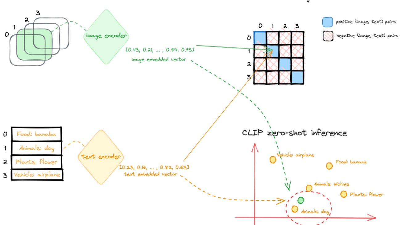
CLIP is a multi-modal vision and language model, which can be used for image-text similarity and for zero-shot image classification. CLIP is trained on a dataset of 400 million image-text pairs collected from a variety of publicly available sources on the internet. The model architecture consists of an image encoder and a text encoder, as shown in the following diagram.

During training, an image and corresponding text snippet are fed through the encoders to get an image feature vector and text feature vector. The goal is to make the image and text features for a matched pair have a high cosine similarity, while features for mismatched pairs have low similarity. This is done through a contrastive loss. This contrastive pre-training results in encoders that map images and text to a common embedding space where semantics are aligned.
The encoders can then be used for zero-shot transfer learning for downstream tasks. At inference time, the image and text pre-trained encoder processes its respective input and transforms it into a high-dimensional vector representation, or an embedding. The embeddings of the image and text are then compared to determine their similarity, such as cosine similarity. The text prompt (image classes, categories, or tags) whose embedding is most similar (for example, has the smallest distance) to the image embedding is considered the most relevant, and the image is classified accordingly.
BLIP model
Another popular multimodality model is BLIP. It introduces a novel model architecture capable of adapting to diverse vision-language tasks and employs a unique dataset bootstrapping technique to learn from noisy web data. BLIP architecture includes an image encoder and text encoder: the image-grounded text encoder injects visual information into the transformer block of the text encoder, and the image-grounded text decoder incorporates visual information into the transformer decoder block. With this architecture, BLIP demonstrates outstanding performance across a spectrum of vision-language tasks that involve the fusion of visual and linguistic information, from image-based search and content generation to interactive visual dialog systems. In a previous post, we proposed a content moderation solution based on the BLIP model that addressed multiple challenges using computer vision unimodal ML approaches.
Use case 1: Zero-shot tag or attribute generation for an ecommerce platform
Ecommerce platforms serve as dynamic marketplaces teeming with ideas, products, and services. With millions of products listed, effective sorting and categorization poses a significant challenge. This is where the power of auto-tagging and attribute generation comes into its own. By harnessing advanced technologies like ML and NLP, these automated processes can revolutionize the operations of ecommerce platforms.
One of the key benefits of auto-tagging or attribute generation lies in its ability to enhance searchability. Products tagged accurately can be found by customers swiftly and efficiently. For instance, if a customer is searching for a “cotton crew neck t-shirt with a logo in front,” auto-tagging and attribute generation enable the search engine to pinpoint products that match not merely the broader “t-shirt” category, but also the specific attributes of “cotton” and “crew neck.” This precise matching can facilitate a more personalized shopping experience and boost customer satisfaction. Moreover, auto-generated tags or attributes can substantially improve product recommendation algorithms. With a deep understanding of product attributes, the system can suggest more relevant products to customers, thereby increasing the likelihood of purchases and enhancing customer satisfaction.
CLIP offers a promising solution for automating the process of tag or attribute generation. It takes a product image and a list of descriptions or tags as input, generating a vector representation, or embedding, for each tag. These embeddings exist in a high-dimensional space, with their relative distances and directions reflecting the semantic relationships between the inputs. CLIP is pre-trained on a large scale of image-text pairs to encapsulate these meaningful embeddings. If a tag or attribute accurately describes an image, their embeddings should be relatively close in this space. To generate corresponding tags or attributes, a list of potential tags can be inputted into the text part of the CLIP model, and the resulting embeddings stored. Ideally, this list should be exhaustive, covering all potential categories and attributes relevant to the products on the ecommerce platform. The following figure shows some examples.

To deploy the CLIP model on SageMaker, you can follow the notebook in the following GitHub repo. We use the SageMaker pre-built large model inference (LMI) containers to deploy the model. The LMI containers use DJL Serving to serve your model for inference. To learn more about hosting large models on SageMaker, refer to Deploy large models on Amazon SageMaker using DJLServing and DeepSpeed model parallel inference and Deploy large models at high performance using FasterTransformer on Amazon SageMaker.
In this example, we provide the files serving.properties, model.py, and requirements.txt to prepare the model artifacts and store them in a tarball file.
serving.propertiesis the configuration file that can be used to indicate to DJL Serving which model parallelization and inference optimization libraries you would like to use. Depending on your need, you can set the appropriate configuration. For more details on the configuration options and an exhaustive list, refer to Configurations and settings.model.pyis the script that handles any requests for serving.requirements.txtis the text file containing any additional pip wheels to install.
If you want to download the model from Hugging Face directly, you can set the option.model_id parameter in the serving.properties file as the model id of a pre-trained model hosted inside a model repository on huggingface.co. The container uses this model id to download the corresponding model during deployment time. If you set the model_id to an Amazon Simple Storage Service (Amazon S3) URL, the DJL will download the model artifacts from Amazon S3 and swap the model_id to the actual location of the model artifacts. In your script, you can point to this value to load the pre-trained model. In our example, we use the latter option, because the LMI container uses s5cmd to download data from Amazon S3, which significantly reduces the speed when loading models during deployment. See the following code:
In the model.py script, we load the model path using the model ID provided in the property file:
After the model artifacts are prepared and uploaded to Amazon S3, you can deploy the CLIP model to SageMaker hosting with a few lines of code:
When the endpoint is in service, you can invoke the endpoint with an input image and a list of labels as the input prompt to generate the label probabilities:
Use case 2: Automatic prompt generation from images
One innovative application using the multimodality models is to generate informative prompts from an image. In generative AI, a prompt refers to the input provided to a language model or other generative model to instruct it on what type of content or response is desired. The prompt is essentially a starting point or a set of instructions that guides the model’s generation process. It can take the form of a sentence, question, partial text, or any input that conveys the context or desired output to the model. The choice of a well-crafted prompt is pivotal in generating high-quality images with precision and relevance. Prompt engineering is the process of optimizing or crafting a textual input to achieve desired responses from a language model, often involving wording, format, or context adjustments.
Prompt engineering for image generation poses several challenges, including the following:
- Defining visual concepts accurately – Describing visual concepts in words can sometimes be imprecise or ambiguous, making it difficult to convey the exact image desired. Capturing intricate details or complex scenes through textual prompts might not be straightforward.
- Specifying desired styles effectively – Communicating specific stylistic preferences, such as mood, color palette, or artistic style, can be challenging through text alone. Translating abstract aesthetic concepts into concrete instructions for the model can be tricky.
- Balancing complexity to prevent overloading the model – Elaborate prompts could confuse the model or lead to overloading it with information, affecting the generated output. Striking the right balance between providing sufficient guidance and avoiding overwhelming complexity is essential.
Therefore, crafting effective prompts for image generation is time consuming, which requires iterative experimentation and refining to strike the right balance between precision and creativity, making it a resource-intensive task that heavily relies on human expertise.
The CLIP Interrogator is an automatic prompt engineering tool for images that combines CLIP and BLIP to optimize text prompts to match a given image. You can use the resulting prompts with text-to-image models like Stable Diffusion to create cool art. The prompts created by CLIP Interrogator offer a comprehensive description of the image, covering not only its fundamental elements but also the artistic style, the potential inspiration behind the image, the medium where the image could have been or might be used, and beyond. You can easily deploy the CLIP Interrogator solution on SageMaker to streamline the deployment process, and take advantage of the scalability, cost-efficiency, and robust security provided by the fully managed service. The following diagram shows the flow logic of this solution.

You can use the following notebook to deploy the CLIP Interrogator solution on SageMaker. Similarly, for CLIP model hosting, we use the SageMaker LMI container to host the solution on SageMaker using DJL Serving. In this example, we provided an additional input file with the model artifacts that specifies the models deployed to the SageMaker endpoint. You can choose different CLIP or BLIP models by passing the caption model name and the clip model name through the model_name.json file created with the following code:
The inference script model.py contains a handle function that DJL Serving will run your request by invoking this function. To prepare this entry point script, we adopted the code from the original clip_interrogator.py file and modified it to work with DJL Serving on SageMaker hosting. One update is the loading of the BLIP model. The BLIP and CLIP models are loaded via the load_caption_model() and load_clip_model() function during the initialization of the Interrogator object. To load the BLIP model, we first downloaded the model artifacts from Hugging Face and uploaded them to Amazon S3 as the target value of the model_id in the properties file. This is because the BLIP model can be a large file, such as the blip2-opt-2.7b model, which is more than 15 GB in size. Downloading the model from Hugging Face during model deployment will require more time for endpoint creation. Therefore, we point the model_id to the Amazon S3 location of the BLIP2 model and load the model from the model path specified in the properties file. Note that, during deployment, the model path will be swapped to the local container path where the model artifacts were downloaded to by DJL Serving from the Amazon S3 location. See the following code:
Because the CLIP model isn’t very big in size, we use open_clip to load the model directly from Hugging Face, which is the same as the original clip_interrogator implementation:
We use similar code to deploy the CLIP Interrogator solution to a SageMaker endpoint and invoke the endpoint with an input image to get the prompts that can be used to generate similar images.
Let’s take the following image as an example. Using the deployed CLIP Interrogator endpoint on SageMaker, it generates the following text description: croissant on a plate, pexels contest winner, aspect ratio 16:9, cgsocietywlop, 8 h, golden cracks, the artist has used bright, picture of a loft in morning, object features, stylized border, pastry, french emperor.

We can further combine the CLIP Interrogator solution with Stable Diffusion and prompt engineering techniques—a whole new dimension of creative possibilities emerges. This integration allows us to not only describe images with text, but also manipulate and generate diverse variations of the original images. Stable Diffusion ensures controlled image synthesis by iteratively refining the generated output, and strategic prompt engineering guides the generation process towards desired outcomes.
In the second part of the notebook, we detail the steps to use prompt engineering to restyle images with the Stable Diffusion model (Stable Diffusion XL 1.0). We use the Stability AI SDK to deploy this model from SageMaker JumpStart after subscribing to this model on the AWS marketplace. Because this is a newer and better version for image generation provided by Stability AI, we can get high-quality images based on the original input image. Additionally, if we prefix the preceding description and add an additional prompt mentioning a known artist and one of his works, we get amazing results with restyling. The following image uses the prompt: This scene is a Van Gogh painting with The Starry Night style, croissant on a plate, pexels contest winner, aspect ratio 16:9, cgsocietywlop, 8 h, golden cracks, the artist has used bright, picture of a loft in morning, object features, stylized border, pastry, french emperor.

The following image uses the prompt: This scene is a Hokusai painting with The Great Wave off Kanagawa style, croissant on a plate, pexels contest winner, aspect ratio 16:9, cgsocietywlop, 8 h, golden cracks, the artist has used bright, picture of a loft in morning, object features, stylized border, pastry, french emperor.

Conclusion
The emergence of multimodality models, like CLIP and BLIP, and their applications are rapidly transforming the landscape of image-to-text conversion. Bridging the gap between visual and semantic information, they are providing us with the tools to unlock the vast potential of visual data and harness it in ways that were previously unimaginable.
In this post, we illustrated different applications of the multimodality models. These range from enhancing the efficiency and accuracy of search in ecommerce platforms through automatic tagging and categorization to the generation of prompts for text-to-image models like Stable Diffusion. These applications open new horizons for creating unique and engaging content. We encourage you to learn more by exploring the various multimodality models on SageMaker and build a solution that is innovative to your business.
About the Authors
 Yanwei Cui, PhD, is a Senior Machine Learning Specialist Solutions Architect at AWS. He started machine learning research at IRISA (Research Institute of Computer Science and Random Systems), and has several years of experience building AI-powered industrial applications in computer vision, natural language processing, and online user behavior prediction. At AWS, he shares his domain expertise and helps customers unlock business potentials and drive actionable outcomes with machine learning at scale. Outside of work, he enjoys reading and traveling.
 Raghu Ramesha is a Senior ML Solutions Architect with the Amazon SageMaker Service team. He focuses on helping customers build, deploy, and migrate ML production workloads to SageMaker at scale. He specializes in machine learning, AI, and computer vision domains, and holds a master’s degree in Computer Science from UT Dallas. In his free time, he enjoys traveling and photography.
 Sam Edwards, is a Cloud Engineer (AI/ML) at AWS Sydney specialized in machine learning and Amazon SageMaker. He is passionate about helping customers solve issues related to machine learning workflows and creating new solutions for them. Outside of work, he enjoys playing racquet sports and traveling.
 Melanie Li, PhD, is a Senior AI/ML Specialist TAM at AWS based in Sydney, Australia. She helps enterprise customers build solutions using state-of-the-art AI/ML tools on AWS and provides guidance on architecting and implementing ML solutions with best practices. In her spare time, she loves to explore nature and spend time with family and friends.
 Gordon Wang is a Senior AI/ML Specialist TAM at AWS. He supports strategic customers with AI/ML best practices cross many industries. He is passionate about computer vision, NLP, generative AI, and MLOps. In his spare time, he loves running and hiking.
 Dhawal Patel is a Principal Machine Learning Architect at AWS. He has worked with organizations ranging from large enterprises to mid-sized startups on problems related to distributed computing, and Artificial Intelligence. He focuses on Deep learning including NLP and Computer Vision domains. He helps customers achieve high performance model inference on SageMaker.
How economic data informs a more equitable employee experience at Amazon
Wharton professor Jessie Handbury lends her expertise to Amazon’s PXTCS Team as an Amazon Visiting Academic.Read More
Improve prediction quality in custom classification models with Amazon Comprehend
Artificial intelligence (AI) and machine learning (ML) have seen widespread adoption across enterprise and government organizations. Processing unstructured data has become easier with the advancements in natural language processing (NLP) and user-friendly AI/ML services like Amazon Textract, Amazon Transcribe, and Amazon Comprehend. Organizations have started to use AI/ML services like Amazon Comprehend to build classification models with their unstructured data to get deep insights that they didn’t have before. Although you can use pre-trained models with minimal effort, without proper data curation and model tuning, you can’t realize the full benefits AI/ML models.
In this post, we explain how to build and optimize a custom classification model using Amazon Comprehend. We demonstrate this using an Amazon Comprehend custom classification to build a multi-label custom classification model, and provide guidelines on how to prepare the training dataset and tune the model to meet performance metrics such as accuracy, precision, recall, and F1 score. We use the Amazon Comprehend model training output artifacts like a confusion matrix to tune model performance and guide you on improving your training data.
Solution overview
This solution presents an approach to building an optimized custom classification model using Amazon Comprehend. We go through several steps, including data preparation, model creation, model performance metric analysis, and optimizing inference based on our analysis. We use an Amazon SageMaker notebook and the AWS Management Console to complete some of these steps.
We also go through best practices and optimization techniques during data preparation, model building, and model tuning.
Prerequisites
If you don’t have a SageMaker notebook instance, you can create one. For instructions, refer to Create an Amazon SageMaker Notebook Instance.
Prepare the data
For this analysis, we use the Toxic Comment Classification dataset from Kaggle. This dataset contains 6 labels with 158,571 data points. However, each label only has less than 10% of the total data as positive examples, with two of the labels having less than 1%.
We convert the existing Kaggle dataset to the Amazon Comprehend two-column CSV format with the labels split using a pipe (|) delimiter. Amazon Comprehend expects at least one label for each data point. In this dataset, we encounter several data points that don’t fall under any of the provided labels. We create a new label called clean and assign any of the data points that aren’t toxic to be positive with this label. Finally, we split the curated datasets into training and test datasets using an 80/20 ratio split per label.
We will be using the Data-Preparation notebook. The following steps use the Kaggle dataset and prepare the data for our model.
- On the SageMaker console, choose Notebook instances in the navigation pane.
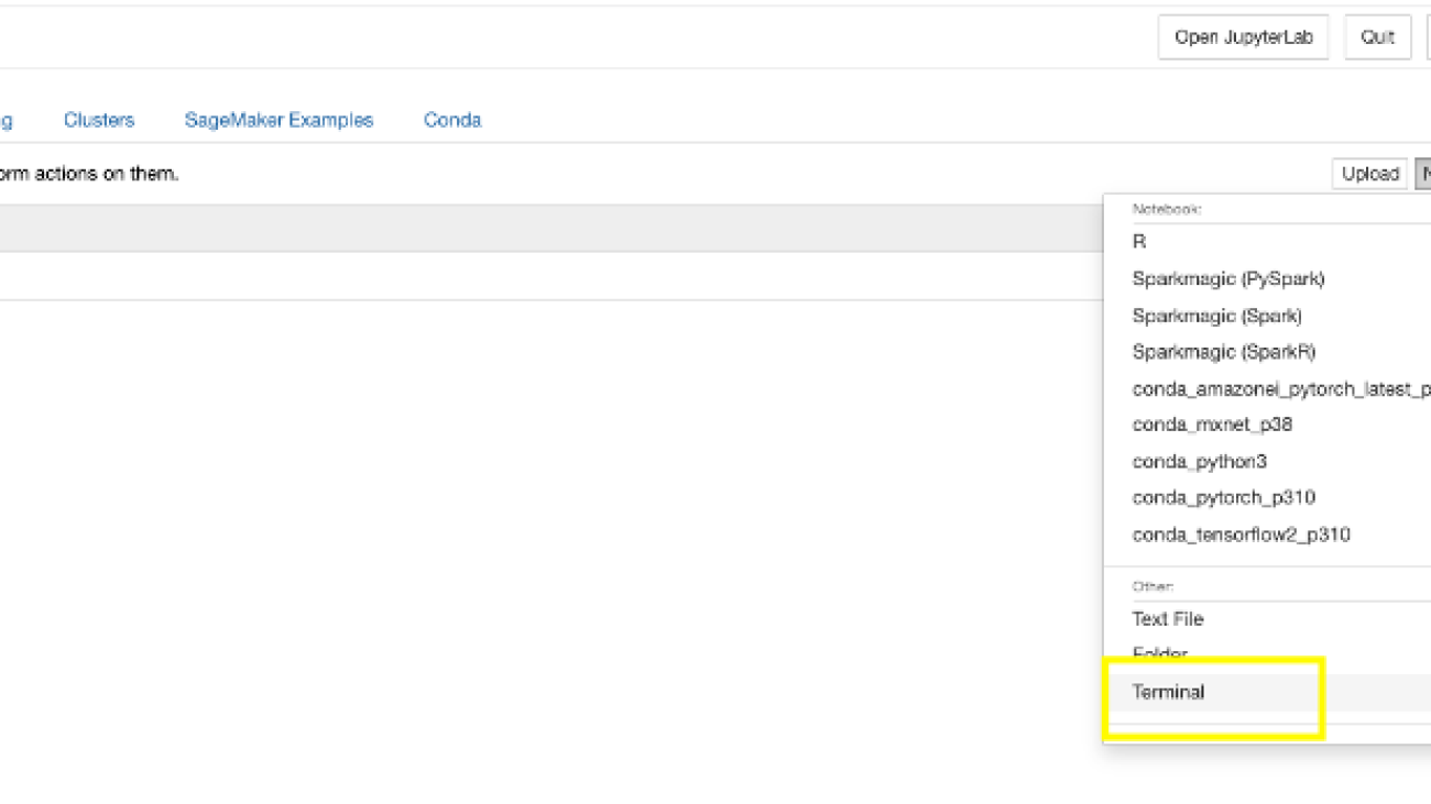
- Select the notebook instance you have configured and choose Open Jupyter.
- On the New menu, choose Terminal.

- Run the following commands in the terminal to download the required artifacts for this post:
- Close the terminal window.
You should see three notebooks and train.csv files.
- Choose the notebook Data-Preparation.ipynb.
- Run all the steps in the notebook.
These steps prepare the raw Kaggle dataset to serve as curated training and test datasets. Curated datasets will be stored in the notebook and Amazon Simple Storage Service (Amazon S3).
Consider the following data preparation guidelines when dealing with large-scale multi-label datasets:
- Datasets must have a minimum of 10 samples per label.
- Amazon Comprehend accepts a maximum of 100 labels. This is a soft limit that can be increased.
- Ensure the dataset file is correctly formatted with the proper delimiter. Incorrect delimiters can introduce blank labels.
- All the data points must have labels.
- Training and test datasets should have balanced data distribution per label. Don’t use random distribution because it might introduce bias in the training and test datasets.
Build a custom classification model
We use the curated training and test datasets we created during the data preparation step to build our model. The following steps create an Amazon Comprehend multi-label custom classification model:
- On the Amazon Comprehend console, choose Custom classification in the navigation pane.
- Choose Create new model.
- For Model name, enter toxic-classification-model.
- For Version name, enter 1.
- For Annotation and data format, choose Using Multi-label mode.
- For Training dataset, enter the location of the curated training dataset on Amazon S3.
- Choose Customer provided test dataset and enter the location of the curated test data on Amazon S3.
- For Output data, enter the Amazon S3 location.
- For IAM role, select Create an IAM role, specify the name suffix as “comprehend-blog”.
- Choose Create to start the custom classification model training and model creation.
The following screenshot shows the custom classification model details on the Amazon Comprehend console.

Tune for model performance
The following screenshot shows the model performance metrics. It includes key metrics like precision, recall, F1 score, accuracy, and more.

After the model is trained and created, it will generate the output.tar.gz file, which contains the labels from the dataset as well as the confusion matrix for each of the labels. To further tune the model’s prediction performance, you have to understand your model with the prediction probabilities for each class. To do this, you need to create an analysis job to identify the scores Amazon Comprehend assigned to each of the data points.
Complete the following steps to create an analysis job:
- On the Amazon Comprehend console, choose Analysis jobs in the navigation pane.
- Choose Create job.
- For Name, enter
toxic_train_data_analysis_job. - For Analysis type, choose Custom classification.
- For Classification models and flywheels, specify
toxic-classification-model. - For Version, specify 1.
- For Input data S3 location, enter the location of the curated training data file.
- For Input format, choose One document per line.
- For Output data S3 location, enter the location.
- For Access Permissions, select Use an existing IAM Role and pick the role created previously.
- Choose Create job to start the analysis job.
- Select the Analysis jobs to view the job details. Please take a note of the job id under Job details. We will be using the job id in our next step.

Repeat the steps to the start analysis job for the curated test data. We use the prediction outputs from our analysis jobs to learn about our model’s prediction probabilities. Please make note of job ids of training and test analysis jobs.
We use the Model-Threshold-Analysis.ipynb notebook to test the outputs on all possible thresholds and score the output based on the prediction probability using the scikit-learn’s precision_recall_curve function. Additionally, we can compute the F1 score at each threshold.
We will need the Amazon Comprehend analysis job id’s as input for Model-Threshold-Analysis notebook. You can get the job ids from Amazon Comprehend console. Execute all the steps in Model-Threshold-Analysis notebook to observe the thresholds for all the classes.

Notice how precision goes up as the threshold goes up, while the inverse occurs with recall. To find the balance between the two, we use the F1 score where it has visible peaks in their curve. The peaks in the F1 score correspond to a particular threshold that can improve the model’s performance. Notice how most of the labels fall around the 0.5 mark for the threshold except for threat label, which has a threshold around 0.04.

We can then use this threshold for specific labels that are underperforming with just the default 0.5 threshold. By using the optimized thresholds, the results of the model on the test data improve for the label threat from 0.00 to 0.24. We are using the max F1 score at the threshold as a benchmark to determine positive vs. negative for that label instead of a common benchmark (a standard value like > 0.7) for all the labels.

Handling underrepresented classes
Another approach that’s effective for an imbalanced dataset is oversampling. By oversampling the underrepresented class, the model sees the underrepresented class more often and emphasizes the importance of those samples. We use the Oversampling-underrepresented.ipynb notebook to optimize the datasets.
For this dataset, we tested how the model’s performance on the evaluation dataset changes as we provide more samples. We use the oversampling technique to increase the occurrence of underrepresented classes to improve the performance.

In this particular case, we tested on 10, 25, 50, 100, 200, and 500 positive examples. Notice that although we are repeating data points, we are inherently improving the performance of the model by emphasizing the importance of the underrepresented class.
Cost
With Amazon Comprehend, you pay as you go based on the number of text characters processed. Refer to Amazon Comprehend Pricing for actual costs.
Clean up
When you’re finished experimenting with this solution, clean up your resources to delete all the resources deployed in this example. This helps you avoid continuing costs in your account.
Conclusion
In this post, we have provided best practices and guidance on data preparation, model tuning using prediction probabilities and techniques to handle underrepresented data classes. You can use these best practices and techniques to improve the performance metrics of your Amazon Comprehend custom classification model.
For more information about Amazon Comprehend, visit Amazon Comprehend developer resources to find video resources and blog posts, and refer to AWS Comprehend FAQs.
About the Authors
 Sathya Balakrishnan is a Sr. Customer Delivery Architect in the Professional Services team at AWS, specializing in data and ML solutions. He works with US federal financial clients. He is passionate about building pragmatic solutions to solve customers’ business problems. In his spare time, he enjoys watching movies and hiking with his family.
 Prince Mallari is an NLP Data Scientist in the Professional Services team at AWS, specializing in applications of NLP for public sector customers. He is passionate about using ML as a tool to allow customers to be more productive. In his spare time, he enjoys playing video games and developing one with his friends.
Fast and cost-effective LLaMA 2 fine-tuning with AWS Trainium
Large language models (LLMs) have captured the imagination and attention of developers, scientists, technologists, entrepreneurs, and executives across several industries. These models can be used for question answering, summarization, translation, and more in applications such as conversational agents for customer support, content creation for marketing, and coding assistants.
Recently, Meta released Llama 2 for both researchers and commercial entities, adding to the list of other LLMs, including MosaicML MPT and Falcon. In this post, we walk through how to fine-tune Llama 2 on AWS Trainium, a purpose-built accelerator for LLM training, to reduce training times and costs. We review the fine-tuning scripts provided by the AWS Neuron SDK (using NeMo Megatron-LM), the various configurations we used, and the throughput results we saw.
About the Llama 2 model
Similar to the previous Llama 1 model and other models like GPT, Llama 2 uses the Transformer’s decoder-only architecture. It comes in three sizes: 7 billion, 13 billion, and 70 billion parameters. Compared to Llama 1, Llama 2 doubles context length from 2,000 to 4,000, and uses grouped-query attention (only for 70B). Llama 2 pre-trained models are trained on 2 trillion tokens, and its fine-tuned models have been trained on over 1 million human annotations.
Distributed training of Llama 2
To accommodate Llama 2 with 2,000 and 4,000 sequence length, we implemented the script using NeMo Megatron for Trainium that supports data parallelism (DP), tensor parallelism (TP), and pipeline parallelism (PP). To be specific, with the new implementation of some features like untie word embedding, rotary embedding, RMSNorm, and Swiglu activation, we use the generic script of GPT Neuron Megatron-LM to support the Llama 2 training script.
Our high-level training procedure is as follows: for our training environment, we use a multi-instance cluster managed by the SLURM system for distributed training and scheduling under the NeMo framework.
First, download the Llama 2 model and training datasets and preprocess them using the Llama 2 tokenizer. For example, to use the RedPajama dataset, use the following command:
For detailed guidance of downloading models and the argument of the preprocessing script, refer to Download LlamaV2 dataset and tokenizer.
Next, compile the model:
After the model is compiled, launch the training job with the following script that is already optimized with the best configuration and hyperparameters for Llama 2 (included in the example code):
Lastly, we monitor TensorBoard to keep track of training progress:
For the complete example code and scripts we mentioned, refer to the Llama 7B tutorial and NeMo code in the Neuron SDK to walk through more detailed steps.
Fine-tuning experiments
We fine-tuned the 7B model on the OSCAR (Open Super-large Crawled ALMAnaCH coRpus) and QNLI (Question-answering NLI) datasets in a Neuron 2.12 environment (PyTorch). For each 2,000 and 4,000 sequence length, we optimized some configurations, such as batchsize and gradient_accumulation, for training efficiency. As a fine-tuning strategy, we adopted full fine-tuning of all parameters (about 500 steps), which can be extended to pre-training with longer steps and larger datasets (for example, 1T RedPajama). Sequence parallelism can also be enabled to allow NeMo Megatron to successfully fine-tune models with a larger sequence length of 4,000. The following table shows the configuration and throughput results of the Llama 7B fine-tuning experiment. The throughput scales almost linearly as the number of instances increase up to 4.
| Distributed Library | Datasets | Sequence Length | Number of Instances | Tensor Parallel | Data Parallel | Pipeline Parellel | Global Batch size | Throughput (seq/s) |
| Neuron NeMo Megatron | OSCAR | 4096 | 1 | 8 | 4 | 1 | 256 | 3.7 |
| . | . | 4096 | 2 | 8 | 4 | 1 | 256 | 7.4 |
| . | . | 4096 | 4 | 8 | 4 | 1 | 256 | 14.6 |
| . | QNLI | 4096 | 4 | 8 | 4 | 1 | 256 | 14.1 |
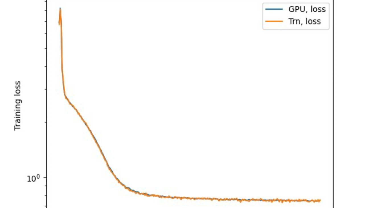
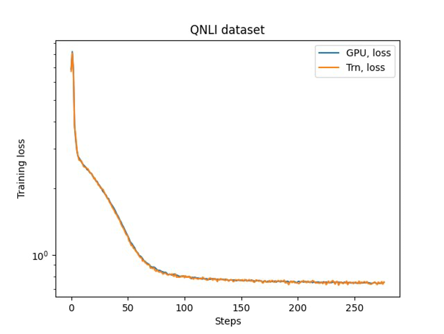
The last step is to verify the accuracy with the base model. We implemented a reference script for GPU experiments and confirmed the training curves for GPU and Trainium matched as shown in the following figure. The figure illustrates loss curves over the number of training steps on the QNLI dataset. Mixed-precision was adopted for GPU (blue), and bf16 with default stochastic rounding for Trainium (orange).
Conclusion
In this post, we showed that Trainium delivers high performance and cost-effective fine-tuning of Llama 2. For more resources on using Trainium for distributed pre-training and fine-tuning your generative AI models using NeMo Megatron, refer to AWS Neuron Reference for NeMo Megatron.
About the Authors
 Hao Zhou is a Research Scientist with Amazon SageMaker. Before that, he worked on developing machine learning methods for fraud detection for Amazon Fraud Detector. He is passionate about applying machine learning, optimization, and generative AI techniques to various real-world problems. He holds a PhD in Electrical Engineering from Northwestern University.
 Karthick Gopalswamy is an Applied Scientist with AWS. Before AWS, he worked as a scientist in Uber and Walmart Labs with a major focus on mixed integer optimization. At Uber, he focused on optimizing the public transit network with on-demand SaaS products and shared rides. At Walmart Labs, he worked on pricing and packing optimizations. Karthick has a PhD in Industrial and Systems Engineering with a minor in Operations Research from North Carolina State University. His research focuses on models and methodologies that combine operations research and machine learning.
 Xin Huang is a Senior Applied Scientist for Amazon SageMaker JumpStart and Amazon SageMaker built-in algorithms. He focuses on developing scalable machine learning algorithms. His research interests are in the area of natural language processing, explainable deep learning on tabular data, and robust analysis of non-parametric space-time clustering. He has published many papers in ACL, ICDM, KDD conferences, and Royal Statistical Society: Series A.
 Youngsuk Park is a Sr. Applied Scientist at AWS Annapurna Labs, working on developing and training foundation models on AI accelerators. Prior to that, Dr. Park worked on R&D for Amazon Forecast in AWS AI Labs as a lead scientist. His research lies in the interplay between machine learning, foundational models, optimization, and reinforcement learning. He has published over 20 peer-reviewed papers in top venues, including ICLR, ICML, AISTATS, and KDD, with the service of organizing workshop and presenting tutorials in the area of time series and LLM training. Before joining AWS, he obtained a PhD in Electrical Engineering from Stanford University.
 Yida Wang is a principal scientist in the AWS AI team of Amazon. His research interest is in systems, high-performance computing, and big data analytics. He currently works on deep learning systems, with a focus on compiling and optimizing deep learning models for efficient training and inference, especially large-scale foundation models. The mission is to bridge the high-level models from various frameworks and low-level hardware platforms including CPUs, GPUs, and AI accelerators, so that different models can run in high performance on different devices.
 Jun (Luke) Huan is a Principal Scientist at AWS AI Labs. Dr. Huan works on AI and Data Science. He has published more than 160 peer-reviewed papers in leading conferences and journals and has graduated 11 PhD students. He was a recipient of the NSF Faculty Early Career Development Award in 2009. Before joining AWS, he worked at Baidu Research as a distinguished scientist and the head of Baidu Big Data Laboratory. He founded StylingAI Inc., an AI start-up, and worked as the CEO and Chief Scientist in 2019–2021. Before joining the industry, he was the Charles E. and Mary Jane Spahr Professor in the EECS Department at the University of Kansas. From 2015–2018, he worked as a program director at the US NSF in charge of its big data program.
 Shruti Koparkar is a Senior Product Marketing Manager at AWS. She helps customers explore, evaluate, and adopt Amazon EC2 accelerated computing infrastructure for their machine learning needs.
How Amazon DataZone helps customers find value in oceans of data
The service, which is now generally available, uses machine learning to make it faster and easier to catalogue, discover, share, and govern data.Read More
Simplify medical image classification using Amazon SageMaker Canvas
Analyzing medical images plays a crucial role in diagnosing and treating diseases. The ability to automate this process using machine learning (ML) techniques allows healthcare professionals to more quickly diagnose certain cancers, coronary diseases, and ophthalmologic conditions. However, one of the key challenges faced by clinicians and researchers in this field is the time-consuming and complex nature of building ML models for image classification. Traditional methods require coding expertise and extensive knowledge of ML algorithms, which can be a barrier for many healthcare professionals.
To address this gap, we used Amazon SageMaker Canvas, a visual tool that allows medical clinicians to build and deploy ML models without coding or specialized knowledge. This user-friendly approach eliminates the steep learning curve associated with ML, which frees up clinicians to focus on their patients.
Amazon SageMaker Canvas provides a drag-and-drop interface for creating ML models. Clinicians can select the data they want to use, specify the desired output, and then watch as it automatically builds and trains the model. Once the model is trained, it generates accurate predictions.
This approach is ideal for medical clinicians who want to use ML to improve their diagnosis and treatment decisions. With Amazon SageMaker Canvas, they can use the power of ML to help their patients, without needing to be an ML expert.
Medical image classification directly impacts patient outcomes and healthcare efficiency. Timely and accurate classification of medical images allows for early detection of diseases that aides in effective treatment planning and monitoring. Moreover, the democratization of ML through accessible interfaces like Amazon SageMaker Canvas, enables a broader range of healthcare professionals, including those without extensive technical backgrounds, to contribute to the field of medical image analysis. This inclusive approach fosters collaboration and knowledge sharing and ultimately leads to advancements in healthcare research and improved patient care.
In this post, we’ll explore the capabilities of Amazon SageMaker Canvas in classifying medical images, discuss its benefits, and highlight real-world use cases that demonstrate its impact on medical diagnostics.
Use case
Skin cancer is a serious and potentially deadly disease, and the earlier it is detected, the better chance there is for successful treatment. Statistically, skin cancer (e.g. Basal and squamous cell carcinomas) is one of the most common cancer types and leads to hundreds of thousands of deaths worldwide each year. It manifests itself through the abnormal growth of skin cells.
However, early diagnosis drastically increases the chances of recovery. Moreover, it may render surgical, radiographic, or chemotherapeutic therapies unnecessary or lessen their overall usage, helping to reduce healthcare costs.
The process of diagnosing skin cancer starts with a procedure called a dermoscopy[1], which inspects the general shape, size, and color characteristics of skin lesions. Suspected lesions then undergo further sampling and histological tests for confirmation of the cancer cell type. Doctors use multiple methods to detect skin cancer, starting with visual detection. The American Center for the Study of Dermatology developed a guide for the possible shape of melanoma, which is called ABCD (asymmetry, border, color, diameter) and is used by doctors for initial screening of the disease. If a suspected skin lesion is found, then the doctor takes a biopsy of the visible lesion on the skin and examines it microscopically for a benign or malignant diagnosis and the type of skin cancer. Computer vision models can play a valuable role in helping to identify suspicious moles or lesions, which enables earlier and more accurate diagnosis.
Creating a cancer detection model is a multi-step process, as outlined below:
- Gather a large dataset of images from healthy skin and skin with various types of cancerous or precancerous lesions. This dataset needs to be carefully curated to ensure accuracy and consistency.
- Use computer vision techniques to preprocess the images and extract relevant to differentiate between healthy and cancerous skin.
- Train an ML model on the preprocessed images, using a supervised learning approach to teach the model to distinguish between different skin types.
- Evaluate the performance of the model using a variety of metrics, such as precision and recall, to ensure that it accurately identifies cancerous skin and minimizes false positives.
- Integrate the model into a user-friendly tool that could be used by dermatologists and other healthcare professionals to aid in the detection and diagnosis of skin cancer.
Overall, the process of developing a skin cancer detection model from scratch typically requires significant resources and expertise. This is where Amazon SageMaker Canvas can help simplify the time and effort for steps 2 – 5.
Solution overview
To demonstrate the creation of a skin cancer computer vision model without writing any code, we use a dermatoscopy skin cancer image dataset published by Harvard Dataverse. We use the dataset, which can be found at HAM10000 and consists of 10,015 dermatoscopic images, to build a skin cancer classification model that predicts skin cancer classes. A few key points about the dataset:
- The dataset serves as a training set for academic ML purposes.
- It includes a representative collection of all important diagnostic categories in the realm of pigmented lesions.
- A few categories in the dataset are: Actinic keratoses and intraepithelial carcinoma / Bowen’s disease (akiec), basal cell carcinoma (bcc), benign keratosis-like lesions (solar lentigines / seborrheic keratoses and lichen-planus like keratoses, bkl), dermatofibroma (df), melanoma (mel), melanocytic nevi (nv) and vascular lesions (angiomas, angiokeratomas, pyogenic granulomas and hemorrhage, vasc)
- More than 50% of the lesions in the dataset are confirmed through histopathology (histo).
- The ground truth for the rest of the cases is determined through follow-up examination (
follow_up), expert consensus (consensus), or confirmation by in vivo confocal microscopy (confocal). - The dataset includes lesions with multiple images, which can be tracked using the
lesion_idcolumn within theHAM10000_metadatafile.
We showcase how to simplify image classification for multiple skin cancer categories without writing any code using Amazon SageMaker Canvas. Given an image of a skin lesion, SageMaker Canvas image classification automatically classifies an image into benign or possible cancer.
Prerequisites
- Access to an AWS account with permissions to create the resources described in the steps section.
- An AWS Identity and Access Management (AWS IAM) user with full permissions to use Amazon SageMaker.
Walkthrough
- Set-up SageMaker domain
- Set-up datasets
- Create an Amazon Simple Storage Service (Amazon S3) bucket with a unique name, which is
image-classification-<ACCOUNT_ID>where ACCOUNT_ID is your unique AWS AccountNumber.
Figure 1 Creating bucket
- In this bucket create two folders:
training-dataandtest-data.
Figure 2 Create folders
- Under training-data, create seven folders for each of the skin cancer categories identified in the dataset:
akiec,bcc,bkl,df,mel,nv, andvasc.
Figure 3 Folder View
- The dataset includes lesions with multiple images, which can be tracked by the
lesion_id-columnwithin theHAM10000_metadatafile. Using thelesion_id-column, copy the corresponding images in the right folder (i.e., you may start with 100 images for each classification).
Figure 4 Listing Objects to import (Sample Images)
- Create an Amazon Simple Storage Service (Amazon S3) bucket with a unique name, which is
- Use Amazon SageMaker Canvas
- Go to the Amazon SageMaker service in the console and select Canvas from the list. Once you are on the Canvas page, please select Open Canvas button.

Figure 5 Navigate to Canvas
- Once you are on the Canvas page, select My models and then choose New Model on the right of your screen.

Figure 6 Creation of Model
- A new pop-up window opens up, where we name image_classify as the model’s name and select Image analysis under the Problem type.
- Go to the Amazon SageMaker service in the console and select Canvas from the list. Once you are on the Canvas page, please select Open Canvas button.
- Import the dataset
- On the next page, please select Create dataset and in the pop-up box name the dataset as image_classify and select the Create button.

Figure 7 Creating dataset
- On the next page, change the Data Source to Amazon S3. You can also directly upload the images (i.e., Local upload).

Figure 8 Import Dataset from S3 buckets
- When you select Amazon S3, you’ll get the list of buckets present in your account. Select the parent bucket that holds the dataset into subfolder (e.g., image-classify-2023 and select Import data button. This allows Amazon SageMaker Canvas to quickly label the images based on the folder names.
- Once, the dataset is successfully imported, you’ll see the value in the Status column change to Ready from Processing.
- Now select your dataset by choosing Select dataset at the bottom of your page.
- On the next page, please select Create dataset and in the pop-up box name the dataset as image_classify and select the Create button.
- Build your model
- On the Build page, you should see your data imported and labelled as per the folder name in Amazon S3.

Figure 9 Labelling of Amazon S3 data
- Select the Quick build button (i.e., the red-highlighted content in the following image) and you’ll see two options to build the model. First one is the Quick build and second one is Standard build. As name suggest quick build option provides speed over accuracy and it takes around 15 to 30 minutes to build the model. The standard build prioritizes accuracy over speed, with model building taking from 45 minutes to 4 hours to complete. Standard build runs experiments using different combinations of hyperparameters and generates many models in the backend (using SageMaker Autopilot functionality) and then picks the best model.
- Select Standard build to start building the model. It takes around 2–5 hours to complete.

Figure 10 Doing Standard build
- Once model build is complete, you can see an estimated accuracy as shown in Figure 11.

Figure 11 Model prediction
- If you select the Scoring tab, it should provide you insights into the model accuracy. Also, we can select the Advanced metrics button on the Scoring tab to view the precision, recall, and F1 score (A balanced measure of accuracy that takes class balance into account).
- The advanced metrics that Amazon SageMaker Canvas shows you depend on whether your model performs numeric, categorical, image, text, or time series forecasting predictions on your data. In this case, we believe recall is more important than precision because missing a cancer detection is far more dangerous than detecting correct. Categorical prediction, such as 2-category prediction or 3-category prediction, refers to the mathematical concept of classification. The advanced metric recall is the fraction of true positives (TP) out of all the actual positives (TP + false negatives). It measures the proportion of positive instances that were correctly predicted as positive by the model. Please refer this A deep dive into Amazon SageMaker Canvas advanced metrics for a deep dive on the advance metrics.

Figure 12 Advanced metrics
This completes the model creation step in Amazon SageMaker Canvas.
- On the Build page, you should see your data imported and labelled as per the folder name in Amazon S3.
- Test your model
- You can now choose the Predict button, which takes you to the Predict page, where you can upload your own images through Single prediction or Batch prediction. Please set the option of your choice and select Import to upload your image and test the model.

Figure 13 Test your own images
- Let’s start by doing a single image prediction. Make sure you are on the Single Prediction and choose Import image. This takes you to a dialog box where you can choose to upload your image from Amazon S3, or do a Local upload. In our case, we select Amazon S3 and browse to our directory where we have the test images and select any image. Then select Import data.

Figure 14 Single Image Prediction
- Once selected, you should see the screen says Generating prediction results. You should have your results in a few minutes as shown below.
- Now let’s try the Batch prediction. Select Batch prediction under Run predictions and select the Import new dataset button and name it BatchPrediction and hit the Create button.

Figure 15 Single image prediction results
- On the next window, make sure you have selected Amazon S3 upload and browse to the directory where we have our test set and select the Import data button.

Figure 16 Batch Image Prediction
- Once the images are in Ready status, select the radio button for the created dataset and choose Generate predictions. Now, you should see the status of batch prediction batch to Generating predictions. Let’s wait for few minutes for the results.
- Once the status is in Ready state, choose the dataset name that takes you to a page showing the detailed prediction on all our images.

Figure 17 Batch image prediction results
- Another important feature of Batch Prediction is to be able to verify the results and also be able to download the prediction in a zip or csv file for further usage or sharing.

Figure 18 Download prediction
- You can now choose the Predict button, which takes you to the Predict page, where you can upload your own images through Single prediction or Batch prediction. Please set the option of your choice and select Import to upload your image and test the model.
With this you have successfully been able to create a model, train it, and test its prediction with Amazon SageMaker Canvas.
Cleaning up
Choose Log out in the left navigation pane to log out of the Amazon SageMaker Canvas application to stop the consumption of SageMaker Canvas workspace instance hours and release all resources.
Citation
[1]Fraiwan M, Faouri E. On the Automatic Detection and Classification of Skin Cancer Using Deep Transfer Learning. Sensors (Basel). 2022 Jun 30;22(13):4963. doi: 10.3390/s22134963. PMID: 35808463; PMCID: PMC9269808.Conclusion
In this post, we showed you how medical image analysis using ML techniques can expedite the diagnosis skin cancer, and its applicability to diagnosing other diseases. However, building ML models for image classification is often complex and time-consuming, requiring coding expertise and ML knowledge. Amazon SageMaker Canvas addressed this challenge by providing a visual interface that eliminates the need for coding or specialized ML skills. This empowers healthcare professionals to use ML without a steep learning curve, allowing them to focus on patient care.
The traditional process of developing a cancer detection model is cumbersome and time-consuming. It involves gathering a curated dataset, preprocessing images, training a ML model, evaluate its performance, and integrate it into a user-friendly tool for healthcare professionals. Amazon SageMaker Canvas simplified the steps from preprocessing to integration, which reduced the time and effort required for building a skin cancer detection model.
In this post, we delved into the powerful capabilities of Amazon SageMaker Canvas in classifying medical images, shedding light on its benefits and presenting real-world use cases that showcase its profound impact on medical diagnostics. One such compelling use case we explored was skin cancer detection and how early diagnosis often significantly enhances treatment outcomes and reduces healthcare costs.
It is important to acknowledge that the accuracy of the model can vary depending on factors, such as the size of the training dataset and the specific type of model employed. These variables play a role in determining the performance and reliability of the classification results.
Amazon SageMaker Canvas can serve as an invaluable tool that assists healthcare professionals in diagnosing diseases with greater accuracy and efficiency. However, it is vital to note that it isn’t intended to replace the expertise and judgment of healthcare professionals. Rather, it empowers them by augmenting their capabilities and enabling more precise and expedient diagnoses. The human element remains essential in the decision-making process, and the collaboration between healthcare professionals and artificial intelligence (AI) tools, including Amazon SageMaker Canvas, is pivotal in providing optimal patient care.
About the authors
 Ramakant Joshi is an AWS Solutions Architect, specializing in the analytics and serverless domain. He has a background in software development and hybrid architectures, and is passionate about helping customers modernize their cloud architecture.
 Jake Wen is a Solutions Architect at AWS, driven by a passion for Machine Learning, Natural Language Processing, and Deep Learning. He assists Enterprise customers in achieving modernization and scalable deployment in the Cloud. Beyond the tech world, Jake finds delight in skateboarding, hiking, and piloting air drones.
 Sonu Kumar Singh is an AWS Solutions Architect, with a specialization in analytics domain. He has been instrumental in catalyzing transformative shifts in organizations by enabling data-driven decision-making thereby fueling innovation and growth. He enjoys it when something he designed or created brings a positive impact. At AWS his intention is to help customers extract value out of AWS’s 200+ cloud services and empower them in their cloud journey.
 Dariush Azimi is a Solution Architect at AWS, with specialization in Machine Learning, Natural Language Processing (NLP), and microservices architecture with Kubernetes. His mission is to empower organizations to harness the full potential of their data through comprehensive end-to-end solutions encompassing data storage, accessibility, analysis, and predictive capabilities.
Create an HCLS document summarization application with Falcon using Amazon SageMaker JumpStart
Healthcare and life sciences (HCLS) customers are adopting generative AI as a tool to get more from their data. Use cases include document summarization to help readers focus on key points of a document and transforming unstructured text into standardized formats to highlight important attributes. With unique data formats and strict regulatory requirements, customers are looking for choices to select the most performant and cost-effective model, as well as the ability to perform necessary customization (fine-tuning) to fit their business use case. In this post, we walk you through deploying a Falcon large language model (LLM) using Amazon SageMaker JumpStart and using the model to summarize long documents with LangChain and Python.
Solution overview
Amazon SageMaker is built on Amazon’s two decades of experience developing real-world ML applications, including product recommendations, personalization, intelligent shopping, robotics, and voice-assisted devices. SageMaker is a HIPAA-eligible managed service that provides tools that enable data scientists, ML engineers, and business analysts to innovate with ML. Within SageMaker is Amazon SageMaker Studio, an integrated development environment (IDE) purpose-built for collaborative ML workflows, which, in turn, contain a wide variety of quickstart solutions and pre-trained ML models in an integrated hub called SageMaker JumpStart. With SageMaker JumpStart, you can use pre-trained models, such as the Falcon LLM, with pre-built sample notebooks and SDK support to experiment with and deploy these powerful transformer models. You can use SageMaker Studio and SageMaker JumpStart to deploy and query your own generative model in your AWS account.
You can also ensure that the inference payload data doesn’t leave your VPC. You can provision models as single-tenant endpoints and deploy them with network isolation. Furthermore, you can curate and manage the selected set of models that satisfy your own security requirements by using the private model hub capability within SageMaker JumpStart and storing the approved models in there. SageMaker is in scope for HIPAA BAA, SOC123, and HITRUST CSF.
The Falcon LLM is a large language model, trained by researchers at Technology Innovation Institute (TII) on over 1 trillion tokens using AWS. Falcon has many different variations, with its two main constituents Falcon 40B and Falcon 7B, comprised of 40 billion and 7 billion parameters, respectively, with fine-tuned versions trained for specific tasks, such as following instructions. Falcon performs well on a variety of tasks, including text summarization, sentiment analysis, question answering, and conversing. This post provides a walkthrough that you can follow to deploy the Falcon LLM into your AWS account, using a managed notebook instance through SageMaker JumpStart to experiment with text summarization.
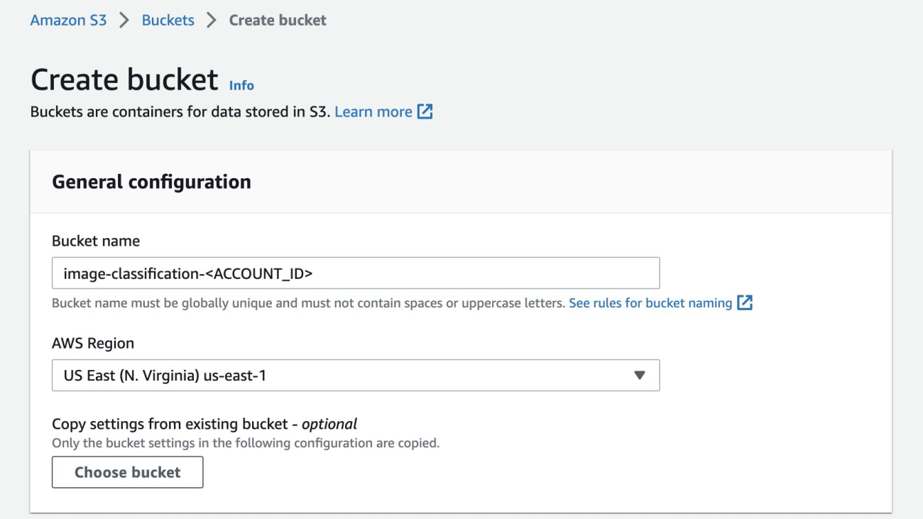
The SageMaker JumpStart model hub includes complete notebooks to deploy and query each model. As of this writing, there are six versions of Falcon available in the SageMaker JumpStart model hub: Falcon 40B Instruct BF16, Falcon 40B BF16, Falcon 180B BF16, Falcon 180B Chat BF16, Falcon 7B Instruct BF16, and Falcon 7B BF16. This post uses the Falcon 7B Instruct model.
In the following sections, we show how to get started with document summarization by deploying Falcon 7B on SageMaker Jumpstart.
Prerequisites
For this tutorial, you’ll need an AWS account with a SageMaker domain. If you don’t already have a SageMaker domain, refer to Onboard to Amazon SageMaker Domain to create one.
Deploy Falcon 7B using SageMaker JumpStart
To deploy your model, complete the following steps:
- Navigate to your SageMaker Studio environment from the SageMaker console.
- Within the IDE, under SageMaker JumpStart in the navigation pane, choose Models, notebooks, solutions.
- Deploy the Falcon 7B Instruct model to an endpoint for inference.

This will open the model card for the Falcon 7B Instruct BF16 model. On this page, you can find the Deploy or Train options as well as links to open the sample notebooks in SageMaker Studio. This post will use the sample notebook from SageMaker JumpStart to deploy the model.
- Choose Open notebook.

- Run the first four cells of the notebook to deploy the Falcon 7B Instruct endpoint.
You can see your deployed JumpStart models on the Launched JumpStart assets page.
- In the navigation pane, under SageMaker Jumpstart, choose Launched JumpStart assets.
- Choose the Model endpoints tab to view the status of your endpoint.

With the Falcon LLM endpoint deployed, you are ready to query the model.
Run your first query
To run a query, complete the following steps:
- On the File menu, choose New and Notebook to open a new notebook.
You can also download the completed notebook here.

- Select the image, kernel, and instance type when prompted. For this post, we choose the Data Science 3.0 image, Python 3 kernel, and ml.t3.medium instance.

- Import the Boto3 and JSON modules by entering the following two lines into the first cell:
- Press Shift + Enter to run the cell.
- Next, you can define a function that will call your endpoint. This function takes a dictionary payload and uses it to invoke the SageMaker runtime client. Then it deserializes the response and prints the input and generated text.
The payload includes the prompt as inputs, together with the inference parameters that will be passed to the model.
- You can use these parameters with the prompt to tune the output of the model for your use case:
Query with a summarization prompt
This post uses a sample research paper to demonstrate summarization. The example text file is concerning automatic text summarization in biomedical literature. Complete the following steps:
- Download the PDF and copy the text into a file named
document.txt. - In SageMaker Studio, choose the upload icon and upload the file to your SageMaker Studio instance.

Out of the box, the Falcon LLM provides support for text summarization.
- Let’s create a function that uses prompt engineering techniques to summarize
document.txt:
You’ll notice that for longer documents, an error appears—Falcon, alongside all other LLMs, has a limit on the number of tokens passed as input. We can get around this limit using LangChain’s enhanced summarization capabilities, which allows for a much larger input to be passed to the LLM.
Import and run a summarization chain
LangChain is an open-source software library that allows developers and data scientists to quickly build, tune, and deploy custom generative applications without managing complex ML interactions, commonly used to abstract many of the common use cases for generative AI language models in just a few lines of code. LangChain’s support for AWS services includes support for SageMaker endpoints.
LangChain provides an accessible interface to LLMs. Its features include tools for prompt templating and prompt chaining. These chains can be used to summarize text documents that are longer than what the language model supports in a single call. You can use a map-reduce strategy to summarize long documents by breaking it down into manageable chunks, summarizing them, and combining them (and summarized again, if needed).
- Let’s install LangChain to begin:
- Import the relevant modules and break down the long document into chunks:
- To make LangChain work effectively with Falcon, you need to define the default content handler classes for valid input and output:
- You can define custom prompts as
PromptTemplateobjects, the main vehicle for prompting with LangChain, for the map-reduce summarization approach. This is an optional step because mapping and combine prompts are provided by default if the parameters within the call to load the summarization chain (load_summarize_chain) are undefined.
- LangChain supports LLMs hosted on SageMaker inference endpoints, so instead of using the AWS Python SDK, you can initialize the connection through LangChain for greater accessibility:
- Finally, you can load in a summarization chain and run a summary on the input documents using the following code:
Because the verbose parameter is set to True, you’ll see all of the intermediate outputs of the map-reduce approach. This is useful for following the sequence of events to arrive at a final summary. With this map-reduce approach, you can effectively summarize documents much longer than is normally allowed by the model’s maximum input token limit.
Clean up
After you’ve finished using the inference endpoint, it’s important to delete it to avoid incurring unnecessary costs through the following lines of code:
Using other foundation models in SageMaker JumpStart
Utilizing other foundation models available in SageMaker JumpStart for document summarization requires minimal overhead to set up and deploy. LLMs occasionally vary with the structure of input and output formats, and as new models and pre-made solutions are added to SageMaker JumpStart, depending on the task implementation, you may have to make the following code changes:
- If you are performing summarization via the
summarize()method (the method without using LangChain), you may have to change the JSON structure of thepayloadparameter, as well as the handling of the response variable in thequery_endpoint()function - If you are performing summarization via LangChain’s
load_summarize_chain()method, you may have to modify theContentHandlerTextSummarizationclass, specifically thetransform_input()andtransform_output()functions, to correctly handle the payload that the LLM expects and the output the LLM returns
Foundation models vary not only in factors such as inference speed and quality, but also input and output formats. Refer to the LLM’s relevant information page on expected input and output.
Conclusion
The Falcon 7B Instruct model is available on the SageMaker JumpStart model hub and performs on a number of use cases. This post demonstrated how you can deploy your own Falcon LLM endpoint into your environment using SageMaker JumpStart and do your first experiments from SageMaker Studio, allowing you to rapidly prototype your models and seamlessly transition to a production environment. With Falcon and LangChain, you can effectively summarize long-form healthcare and life sciences documents at scale.
For more information on working with generative AI on AWS, refer to Announcing New Tools for Building with Generative AI on AWS. You can start experimenting and building document summarization proofs of concept for your healthcare and life science-oriented GenAI applications using the method outlined in this post. When Amazon Bedrock is generally available, we will publish a follow-up post showing how you can implement document summarization using Amazon Bedrock and LangChain.
About the Authors
 John Kitaoka is a Solutions Architect at Amazon Web Services. John helps customers design and optimize AI/ML workloads on AWS to help them achieve their business goals.
 Josh Famestad is a Solutions Architect at Amazon Web Services. Josh works with public sector customers to build and execute cloud based approaches to deliver on business priorities.
Automate prior authorization using CRD with CDS Hooks and AWS HealthLake
Prior authorization is a crucial process in healthcare that involves the approval of medical treatments or procedures before they are carried out. This process is necessary to ensure that patients receive the right care and that healthcare providers are following the correct procedures. However, prior authorization can be a time-consuming and complex process that requires a lot of paperwork and communication between healthcare providers, insurance companies, and patients.
The prior authorization process for electronic health record (EHRs) consists of five steps:
- Determine whether prior authorization is required.
- Gather information necessary to support the prior authorization request.
- Submit the request for prior authorization.
- Monitor the prior authorization request for resolution.
- If needed, supplement the prior authorization request with additional required information (and resume at Step 4).
The Da Vinci Burden Reduction project has rearranged these steps for prior authorization into three interrelated implementation guides that are focused on reducing the clinician and payer burden:
- Coverage Requirements Discovery (CRD) – This provides decision support to providers at the time they’re ordering diagnostics, specifying treatments, making referrals, scheduling appointments, and so on.
- Documentation Templates and Rules (DTR) – This allows providers to download smart questionnaires and rules, such as Clinical Quality Language (CQL), and provides a SMART on FHIR app or EHR app that runs the questionnaires and rules to gather information relevant to a performed or planned service. Running the questionnaires and rules may also be performed by an application that is part of the provider’s EHR.
- Prior Authorization Support (PAS) – This allows provider systems to send (and payer systems to receive) prior authorization requests using FHIR, while still meeting regulatory mandates to have X12 278 used, where required, to transport the prior authorization, potentially simplifying processing for either exchange partner (or both).
In this post, we focus on the CRD implementation guide to determine prior authorization requirements and explain how CDS (Clinical Decision Support) Hooks uses AWS HealthLake to determine if prior authorization is required or not.
Solution overview
CRD is a protocol within the electronic prior authorization workflow that facilitates calls between EHRs and the payers using CDS services. When utilized, it provides information on coverage requirements to providers while patient care decisions are in progress. This enables provider staff to make more informed decisions and meet the requirements of their patient’s insurance coverage. Interaction between providers and payers is done seamlessly using CDS Hooks.
CDS Hooks is a Health Level Seven International (HL7) specification. CDS Hooks provides a way to embed additional, near-real-time functionality within a clinician’s workflow of an EHR. With CDS Hooks, eligibility practices like prior authorization can be properly optimized, along with other pre-certification requirements like the physician’s network participation. This function assists providers in making informed decisions by providing them with information on their patient’s condition, treatment options, and the forms that must be completed to facilitate their care. The strategic use of CDS Hooks allows clinicians to quickly develop more patient-centered care plans and assist the prior authorization process by disclosing critical administrative and clinical requirements. For more information on CDS Hooks and its specification, refer to the CDS Hooks website.
The following diagram illustrates how the CRD workflow is automated using HealthLake.

The workflow steps are as follows:
- A provider staff member logs into the EHR system to open the patient chart.
- The EHR system validates user credentials and invokes the patient-view hook to retrieve patient condition information.
- Amazon API Gateway invokes the Patient View Hooks AWS Lambda function.
- The Lambda function validates and retrieves the patient ID from the request and gets the patient condition information from HealthLake.
- After reviewing the patient condition, the user invokes the order-select hook to retrieve coverage requirements information for the respective drug.
- API Gateway invokes the Coverage Requirements Hooks Lambda function.
- The Lambda function retrieves claims information for the patient, runs CQL rules based on the medication submitted and claims information retrieved from HealthLake, and determines whether prior authorization is required.
The solution is available in the Determine Coverage Requirements Discovery using CDS Hooks with AWS HealthLake GitHub repo.
Prerequisites
This post assumes familiarity with the following services:
- API Gateway
- HealthLake
- Lambda
- AWS Serverless Application Model (AWS SAM)
Deploy the application using the AWS SAM CLI
You can deploy the template using the AWS Management Console or the AWS SAM CLI. To use the CLI, complete the following steps:
- Install the AWS SAM CLI.
- Download the sample code from the AWS samples repository to your local system:
git clone https://github.com/aws-samples/aws-crd-hooks-with-awshealthlake-api
cd aws-crd-hooks-with-awshealthlake-api/- Build the application using AWS SAM:
sam build- Deploy the application using the guided process:
sam deploy --guided
# Replace MY_VALUE with proper resource names
Configuring SAM deploy

======================

Looking for config file [samconfig.toml] : Not found

Setting default arguments for 'sam deploy'

     =========================================

     Stack Name [sam-app]: aws-cds-hooks-with-healthlake

     AWS Region [us-east-1]: us-east-2

     #Shows you resources changes to be deployed and require a 'Y' to initiate deploy

     Confirm changes before deploy [y/N]:

     #SAM needs permission to be able to create roles to connect to the resources in your template

     Allow SAM CLI IAM role creation [Y/n]:

     #Preserves the state of previously provisioned resources when an operation fails

     Disable rollback [y/N]:

     cdsDemoServicesFunction has no authentication. Is this okay? [y/N]: y

     cqlQueryFunction has no authentication. Is this okay? [y/N]: y

     cqlQueryOrderFunction has no authentication. Is this okay? [y/N]: y

     Save arguments to configuration file [Y/n]: y

     SAM configuration file [samconfig.toml]:

     SAM configuration environment [default]:
The deployment may take 30 minutes or more while AWS creates a HealthLake data store and related resources in your AWS account. AWS SAM may time out and return you to your command line. This timeout stops AWS SAM from showing you the progress in the cloud, but doesn’t stop the deployment happening in the cloud. If you see a timeout, go to the AWS CloudFormation console and verify the CloudFormation stack deployment status. Integrate CDS Hooks with your clinical workflow when the CloudFormation stack deployment is complete.
Determine coverage requirements for prior authorization
The solution has two hooks, patient-view and order-select, to determine if prior authorization is required or not based on prior authorization rules from payer. CQL is used to evaluate prior authorization rules.
CDS Hooks can be integrated with EHR that supports CDS Hooks. Alternatively, if you don’t have EHR available for testing, you can use the publicly available sandbox as described in the GitHub repo. Note that the CDS Hooks sandbox is being used solely for the purpose of testing.
After your hooks are integrated with EHR, when a user navigates to the clinical workflow, the patient-view hook is run for the configured patient. Note that the patient ID from the clinical workflow should exist in HealthLake. The cards returned from the API indicate that the patient has a sinus infection health condition and the doctor may need to order a prescription.

You can navigate to the RX View tab to order a prescription. Acting as the doctor, choose the appropriate medication and enter other details as shown in the following screenshot.
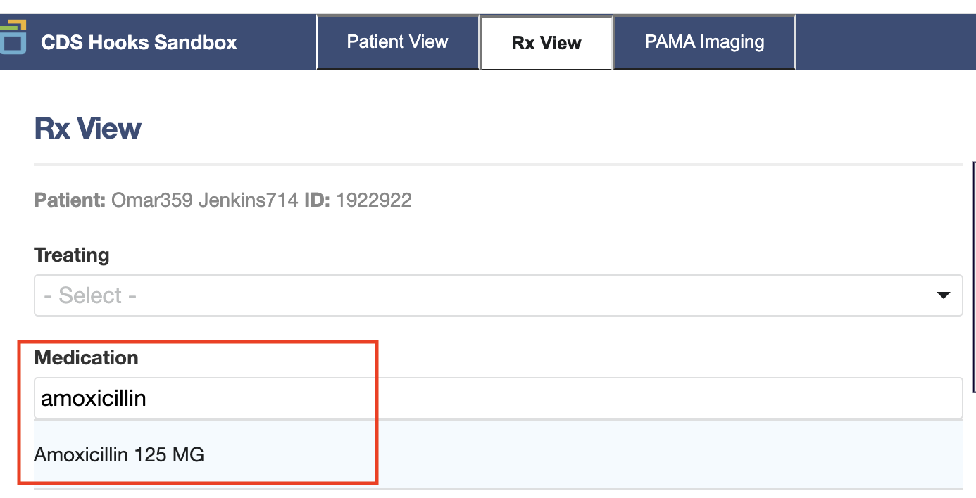
The order-select hook is returned with the prior authorization eligibility card.
The next step is to submit a prior authorization using the SMART app or other mechanisms available to the provider.
Clean up
If you no longer need the AWS resources that you created by running this example, you can remove them by deleting the CloudFormation stack that you deployed:
sam delete --stack-name <<your-stack-name>>Conclusion
In this post, we showed how HealthLake with CDS Hooks can help reduce the burden on providers and improve the member experience by determining coverage requirements for prior authorization as part of the prescription order clinical workflow. CDS Hooks along with HealthLake can help providers at the time they’re ordering diagnostics, specifying treatments, making referrals, and scheduling appointments.
If you are interested in implementing a coverage requirement discovery on AWS using this solution or want to learn more about the implementing prior authorization on AWS , you can contact an AWS Representative.
About the Authors
![]() Manish Patel, a Global Partner Solutions Architect supporting Healthcare and Life Sciences at AWS. He has more than 20 years of experience building solutions for Medicare, Medicaid, Payers, Providers and Life Sciences customers. He drives go-to-market strategies along with partners to accelerate solution developments in areas such as Electronics Health Records, Medical Imaging, multi-model data solutions and Generative AI. He is passionate about using technology to transform the healthcare industry to drive better patient care outcomes.
Manish Patel, a Global Partner Solutions Architect supporting Healthcare and Life Sciences at AWS. He has more than 20 years of experience building solutions for Medicare, Medicaid, Payers, Providers and Life Sciences customers. He drives go-to-market strategies along with partners to accelerate solution developments in areas such as Electronics Health Records, Medical Imaging, multi-model data solutions and Generative AI. He is passionate about using technology to transform the healthcare industry to drive better patient care outcomes.
 Shravan Vurputoor is a Senior Solutions Architect at AWS. As a trusted customer advocate, he helps organizations understand best practices around advanced cloud-based architectures, and provides advice on strategies to help drive successful business outcomes across a broad set of enterprise customers through his passion for educating, training, designing, and building cloud solutions.
New contrastive-learning methods for better data representation
New loss functions enable better approximation of the optimal loss and more-useful representations of multimodal data.Read More