Generative AI is revolutionizing the way developers approach programming by providing intelligent assistance and automation throughout the coding process. With the power of advanced language models and machine learning (ML) algorithms, generative AI can understand the context and intent behind a programmer’s code, offering valuable suggestions, completing code snippets, and even generating entire functions or modules based on high-level descriptions. This technology empowers developers to focus on higher-level problem-solving and architecture, while the AI handles the tedious and repetitive aspects of coding. One of the key advantages of large language models (LLMs) in programming is their ability to learn from the vast amounts of existing code and programming patterns they were trained on. This knowledge allows them to generate context-aware code, detect potential bugs or vulnerabilities, and offer optimizations to improve code quality and performance.
In this post, we highlight how the AWS Generative AI Innovation Center collaborated with SailPoint Technologies to build a generative AI-based coding assistant that uses Anthropic’s Claude Sonnet on Amazon Bedrock to help accelerate the development of software as a service (SaaS) connectors.
Amazon Bedrock is a fully managed service that offers a choice of high-performing foundation models (FMs) from leading AI companies like AI21 Labs, Anthropic, Cohere, Meta, Mistral AI, Stability AI, and Amazon through a single API, along with a broad set of capabilities to build generative AI applications with security, privacy, and responsible AI.
SailPoint specializes in enterprise identity security solutions. Over 3,000 enterprises worldwide use SailPoint to help defend against today’s dynamic, identity-centric cyber threats while enhancing productivity and efficiency. Their products are designed to manage and secure access to applications and data through the lens of identity, at speed and scale, for users inside an organization and for external parties such as non-employees. SailPoint’s unified, intelligent, and extensible environment provides comprehensive identity governance capabilities, including access certifications, policy management, access request and provisioning, password management, and data access governance. This helps organizations make sure the right individuals have the right access to the right resources at the right times, thereby enforcing security policies and compliance requirements. Founded in 2005, SailPoint has grown to be a key player in identity security, serving customers globally across various industries.
SailPoint connectors and SaaS connectivity
SailPoint’s identity security solutions interface with various software as a service (SaaS) applications to retrieve the necessary information, such as account and access information, from an identity security standpoint. Each SaaS application implements these functionalities in slightly different ways and might expose their implementation through REST-based web APIs that are typically supported by OpenAPI specifications. SailPoint connectors are TypeScript modules that interface with a SaaS application and map the relevant identity security information (such as accounts and entitlements) to a standardized format understood by SailPoint. Based on the APIs exposed by the application, SailPoint connectors can create, update, and delete access on those accounts. SailPoint connectors help manage user identities and their access rights across different environments within an organization, supporting the organization’s compliance and security efforts.
Although a typical connector exposes several functions, for this post, we focus on developing the list user function of a connector that connects to an API endpoint for listing users, retrieving all the users, and transforming them into the format required by SailPoint.
In the following sections, we detail how we used Anthropic’s Claude Sonnet on Amazon Bedrock to automatically create the list user connector, a critical component of the broader SaaS connectivity.
Understanding the list user connector
Connectors are modules that can connect to an external service and retrieve and update relevant information from a SaaS application. To better understand how connectors are built, we give an example of the connector function that connects to DocuSign’s REST API’s getUsers endpoint. The following TypeScript code defines an asynchronous function listUsers that retrieves a list of user accounts from an external API and constructs a structured output for each user:
// imports
import { Context, Response, StdAccountListHandler, StdAccountListOutput } from '@sailpoint/connector-sdk';

const listUsers: StdAccountListHandler = async (context: Context, input: undefined, res: Response<StdAccountListOutput>) => {
    // retrieve api key and host url from context
    let apiKey = context.apiKey;
    let hostUrl = context.hostUrl;
    let hasMore = true;

    // url construction
    let url = `https://${hostUrl}/Management/v2/organizations/${context.organizationId}/users`;

    // loop through pages
    while (hasMore) {
        // fetch response from the endpoint
        let response = await fetch(url, {
          headers: {
            'Authorization': `Bearer ${apiKey}`
          }
        });
        let results = await response.json();

        // processing users from response
        let users = results.users;
        for (const user of users) {
            const output: StdAccountListOutput = {
                identity: user.id,
                attributes: {
                    user_name: user.user_name,
                    first_name: user.first_name,
                    last_name: user.last_name,
                    user_status: user.user_status,
                    membership_status: user.membership_status,
                    email: user.email,
                    created_on: user.created_on,
                    membership_created_on: user.membership_created_on,
                    ds_group_id: user.company_groups.map(group => group.ds_group_id),
                    ds_group_account_id: user.company_groups.map(group => group.ds_group_account_id)
                }
            };
        }
        // pagination
        if (results.paging.next) {
          url = results.paging.next;
        } else {
          hasMore = false;
        }
    }
}
The following is a breakdown of what each part of the code does:
- Imports – The code imports several types and interfaces from
@sailpoint/connector-sdk. These include Context, Response, StdAccountListHandler, and StdAccountListOutput, which are used to handle the input and output of the function in a standardized way within a SailPoint environment.
- Function definition –
listUsers is defined as an asynchronous function compatible with the StdAccountListHandler It uses the Context to access configuration details like API keys and the base URL, and a Response to structure the output.
- Retrieve API key and host URL – These are extracted from the
context parameter. They are used to authenticate and construct the request URL.
- URL construction – The function constructs the initial URL using the hostUrl and
organizationId from the context. This URL points to an endpoint that returns users associated with a specific organization.
- Loop through pages – The
while loop continues as long as there are more pages of data (hasMore is true). It serves the following functions:
- Fetch data – Inside the
while loop, a fetch request is made to the API endpoint. The request includes an Authorization header that uses the apiKey. The API’s response is converted to JSON format.
- Process users – Inside the
while loop, it extracts user data from the API response. The process loops through each user, constructing an StdAccountListOutput object for each one. This object includes user identifiers and attributes like user names, names, status, email, and group IDs.
- Pagination – Inside the while loop, it checks if there is a next page URL in the pagination information (
results.paging.next). If it exists, it updates the url for the next iteration of the loop. If not, it sets hasMore to false to stop the loop.
Understanding this example helps us understand the step-by-step process of building this function in a connector. We aim to reproduce this process using an LLM with a prompt chaining strategy.
Generate a TypeScript connector using an LLM prompt chain
There are several approaches to using pre-trained LLMs for code generation, with varying levels of complexity:
- Single prompt – You can use models like Anthropic’s Claude to generate code by direct prompting. These models can generate code in a variety of languages, including TypeScript, but they don’t inherently possess domain-specific knowledge relevant to the task of building a connector. All the required information, including API specifications and formatting instructions, must be provided in the prompt, similar to the instructions that would be given to a developer. However, LLMs tend to struggle when given a long list of complex instructions. It’s also difficult for the prompt engineer to understand which steps are challenging for the LLM.
- Agentic frameworks with LLMs – Agents are a sophisticated framework that can use tools to perform a sequence of complex tasks. In this case, the agent starts by breaking down the user requests into steps, searches for necessary information using tools (a knowledge base or web browser), and autonomously generates code from start to finish. Although they’re powerful, these frameworks are complex to implement, often unstable in their behavior, and less controllable compared to other methods. Agents also require many LLM calls to perform a task, which makes them rather slow in practice. In the case where the logic to perform a task is a fixed sequence of steps, agents are not an efficient option.
- Prompt chain – A solution that finds a good trade-off between the two previous approaches involves using a prompt chaining technique. This method breaks the complex problem into a series of more manageable steps and integrates them to craft the final code. Each step has clear instructions that are easier for the LLM to follow, and a human in the loop can control the output of each step and correct the LLM if needed. This approach strikes a balance between flexibility and control, avoiding the extremes of the other two methods.
We initially tested the LLM’s ability to generate connector code based on a single prompt and realized that it struggles to generate code that addresses all aspects of the problem, such as pagination or nested data structures. To make sure the LLM would cover all the necessary components of the connector functions, and because creating a connector follows a fixed sequence of steps, prompt chaining was the most natural approach to improve the generated code.
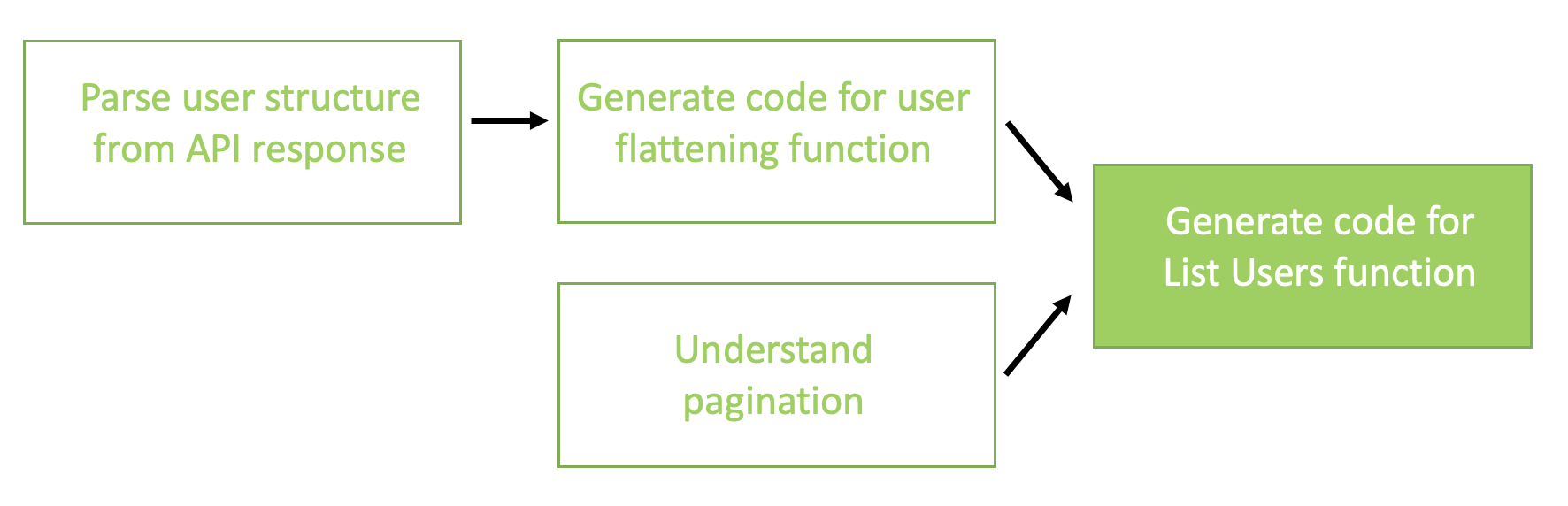
The chain we used for connector generation consists of the following high-level steps:
- Parse the data model of the API response into prescribed TypeScript classes.
- Generate the function for user flattening in the format expected by the connector interface.
- Understand the pagination of the API specs and formulate a high-level solution.
- Generate the code for the
ListUsers function by combining all the intermediate steps.
Step 1 is used as an input to Step 2, but Step 3 is separate. Both Step 2 and Step 3 results are fed to Step 4 for the final result. The following diagram illustrates this workflow.
In the following sections, we will dive into the prompting techniques we used for each of these steps.
System prompt
The system prompt is an essential component of LLM prompting that typically provides the initial context to guide the model’s response. For all the prompts in the chain, we used the following system prompt:
"""
You are an expert web developer who has an excellent understanding of REST APIs and backend
API development using TypeScript. Your goal is to understand API specification provided in
OpenAPI specification or Swagger specification as YAML files and to write TypeScript code,
XML, API descriptions etc. as requested in the task description. Do not deviate from the
provided specification and documentation and if something is unclear in the specification then
mention your uncertainty in the comments do not make up information that is not available in
the specs or description.

When writing TypeScript code, provide minimal but meaningful comments.
"""
More specifically, the system prompt is used to establish the role of the LLM (expert web developer), give it a general goal (understand API specs and write TypeScript code), give high-level instructions (add comments in the code) and set boundaries (do not make up information).
Data model parsing
In this step, we prompt the LLM to understand the structure of the API response and create TypeScript classes corresponding to the objects in the response. Although this step isn’t strictly necessary for generating the response, it can help the LLM immensely in generating a correct connector. Similar to chain-of-thought reasoning for arithmetic problems, it is forcing the LLM to “think” before responding.
This step offers two primary benefits:
- Verbose API response simplification – API responses specified in the documentation can be quite verbose. By converting the response structure into TypeScript classes, we compress the information into fewer lines of code, making it more concise and less complicated for the LLM to comprehend. This step helps ensure that the essential information is prominently displayed at the start.
- Handling fragmented user responses – In some APIs, the user response is composed of several fragments because of the reuse of data structures. The OpenAPI specification uses the
$ref tag to reference these reusable components. By converting the user response into TypeScript classes, we can consolidate all the relevant information into a single location. This consolidation simplifies the downstream steps by providing a centralized source of information.
We use the following task prompt to convert the API response into prescribed TypeScript classes:
"""
You are given an API spec of OpenAPI or Swagger for a REST API endpoint
that serves a list of users for Software as a Service (SaaS) application. You will
be asked to extract the structure of the User in the JSON response from the API endpoint.

Here is the API spec provided between the XML tags <api-spec> </api-spec>.
Understand and remember the API spec well.

<api-spec>
{api_spec}
</api-spec>

Use the following instructions to create TypeScript interfaces based on the structure
of the User.
<instructions>
- Provide the code in between <data-model> </data-model> XML tags.
- If there are any nested objects, expand them into their own interfaces.
- Be comprehensive and include all attributes.
- Retrieve all attributes, including those marked as not mandatory, not required, or nullable.
- The attributes are listed under `properties` section.
- Output only one User interface that includes all the attributes from any interfaces it extends.
</instructions>

The expected format of the output is as follows:
<data-model>
// User
interface User {{
  id: number;
  first_name: string;
  last_name: string;
  email: string;
  is_active: boolean;
  company_groups_ids: number[];
  other_attribute: string;
  nested_type: NestedType[];
}}

// Some complex type
interface NestedType {{
    type_id: string;
    some_string_attribute: string;
    some_number_attribute: number;
}}

</data-model>
"""
In the preceding prompt template, the variable {api_spec} is replaced with the API specification of the endpoint. A specific example for a DocuSign ListUsers endpoint is provided in the appendix.
The following code is an example of the LLM-generated classes when applied to the DocuSign API specs. This has been parsed out of the <data-model> tags.
// User
interface User {
    id: string; // format: uuid
    user_name: string;
    first_name: string;
    last_name: string;
    user_status: string; // One of: 'active' | 'created' | 'closed'
    membership_status: string; // One of: 'activation_required' | 'activation_sent' | 'active' | 'closed' | 'disabled'
    email: string;
    created_on: string; // format: date-time
    membership_created_on: string; // format: date-time
    ds_groups: DsGroup[];
}

// DsGroup
interface DsGroup {
    ds_group_id: string; // format: uuid
    account_id: string; // format: uuid
    source_product_name: string;
    group_id: string;
    group_name: string;
    description: string;
    is_admin: boolean;
    last_modified_on: string; // format: date-time
    user_count: number; // format: int32
    external_account_id: number; // format: int64
    account_name: string;
    membership_id: string; // format: uuid
}
User flattening function generation
The expected structure for each user is an object consisting of two properties: an identifier and a dictionary of attributes. The attributes dictionary is a map that associates string keys with either primitive attributes (number, Boolean, or string) or an array of primitive attributes. because of the potential for arbitrarily nested JSON object structures in the response, we use the capabilities of an LLM to generate a user flattening and conversion function. Both the user ID and the attributes are extracted from the response. By employing this approach, we effectively separate the intricate task of converting the user structure from the REST API response into the required format for the SailPoint connector SDK (hereafter referred to as the connector SDK).
The benefits of this approach are twofold. First, it allows for a cleaner and more modular code design, because the complex conversion process is abstracted away from the main code base. Second, it enables greater flexibility and adaptability, because the conversion function can be modified or regenerated to accommodate changes in the API response structure or the connector SDK requirements, without necessitating extensive modifications to the surrounding code base.
We use the following prompt to generate the conversion function, which takes as input the data model generated in the previous step:
"""
Understand and remember the following data model provided
as a set of TypeScript class definitions.
You will be required to generate a TypeScript function based on the
data model provided between <data-model> </data-model> XML tags.

<data-model>
{data_model}
</data-model>

DO NOT use the TypeScript interfaces defined above in the code you write,
as they will be unavailable. Substitute them with the type `any` where required
to write code that works with strict TypeScript.

Given the TypeScript class definitions and data model above, your goals is to
write a TypeScript function that transforms the user into an object containing two
keys - an `identity` and `attributes`. The attributes is a list of attributes
other than the identifier attribute.

Here are the rules for mapping attributes from the user object to attributes field:

<instructions-for-mapping>
- The function takes in a user and return StdAccountListOutput.
- Extract all attributes specified in the user schema above in the <data-model>
- attributes can only contain either primitives values or array of primitive values.
- Determine the type of the attribute from the <data-model> above. Do not guess it from the
names of the attributes. E.g. if the name is plural don't assume it is an array.
- All primitive attributes such as string and numbers are copied without transformation.
- All arrays of primitive attributes are copied without transformation.
- All objects are flattened out and their attributes are copied as simple attributes.
- All arrays of objects are converted into multiple attributes where each attribute is an array of primitive type.
See further instruction below between the XML tags <object-array-instructions>.
- Use `any` type in functions and arrow function definitions so that it works with TypeScript.
</instructions-for-mapping>


<object-array-instructions>

Consider the following structure of the response where `obj_array` is an attribute that is array of objects of type `MyObj`.
Then in the flattening process, for the response, you will need to convert the `obj_array` attribute
into multiple attributes like `obj_array_attribute1`, `obj_array_attribute2` each of which is an array of strings in this case.

interface User {{
  id: string; // format: uuid
  user_name: string;
  first_name: string;
  obj_array: MyObject[];
}}

interface MyObj {{
  attribute1: string; // format: uuid
  attribute2: string; // format: uuid
  attribute3: string;
}}
 </object-array-instructions>


Output the code according to the template program below enclosed between the <user-mapping-function> XML tags.

This function is part of a larger program so keep the StdAccountListOutput in the function as it is.
Do not overcomplicate and write simple, well readable code.

<user-mapping-function>

function flattenUser(user: any): StdAccountListOutput {{
  return {{
    identity: user.id,
    attributes: {{
      first_name: user.first_name,
      last_name: user.last_name,
      user_type: user.type,
      login: user.login,
      email: user.email,
      location: user.location,
      employee_id: user.employee_id,
      reviewer_id: user.reviewer_id,
      is_active: user.is_active,
      struct_array_attribute: user.struct_array.map( (val: any) => val.struct_attribute)
    }}
  }}
}};

</user-mapping-function>
"""
In the preceding prompt template, we replace the {data_model} variable with the data model of TypeScript classes extracted in the previous generation step of parsing the data model.
The following code is an example of the LLM-generated user flattening function when applied to the DocuSign API:
function flattenUser(user: any): StdAccountListOutput {
    const identity = user.id;
    const attributes: { [key: string]: any } = {};

    // Copy primitive attributes
    attributes.user_name = user.user_name;
    attributes.first_name = user.first_name;
    attributes.last_name = user.last_name;
    attributes.user_status = user.user_status;
    attributes.membership_status = user.membership_status;
    attributes.email = user.email;
    attributes.created_on = user.created_on;
    attributes.membership_created_on = user.membership_created_on;

    // Convert array of objects to multiple attributes
    const dsGroupAttributes: { [key: string]: any[] } = {};
    user.ds_groups.forEach((dsGroup: any) => {
      dsGroupAttributes.ds_group_id = dsGroupAttributes.ds_group_id || [];
      dsGroupAttributes.ds_group_id.push(dsGroup.ds_group_id);

      dsGroupAttributes.account_id = dsGroupAttributes.account_id || [];
      dsGroupAttributes.account_id.push(dsGroup.account_id);

      dsGroupAttributes.source_product_name = dsGroupAttributes.source_product_name || [];
      dsGroupAttributes.source_product_name.push(dsGroup.source_product_name);

      dsGroupAttributes.group_id = dsGroupAttributes.group_id || [];
      dsGroupAttributes.group_id.push(dsGroup.group_id);

      dsGroupAttributes.group_name = dsGroupAttributes.group_name || [];
      dsGroupAttributes.group_name.push(dsGroup.group_name);

      dsGroupAttributes.description = dsGroupAttributes.description || [];
      dsGroupAttributes.description.push(dsGroup.description);

      dsGroupAttributes.is_admin = dsGroupAttributes.is_admin || [];
      dsGroupAttributes.is_admin.push(dsGroup.is_admin);

      dsGroupAttributes.last_modified_on = dsGroupAttributes.last_modified_on || [];
      dsGroupAttributes.last_modified_on.push(dsGroup.last_modified_on);

      dsGroupAttributes.user_count = dsGroupAttributes.user_count || [];
      dsGroupAttributes.user_count.push(dsGroup.user_count);

      dsGroupAttributes.external_account_id = dsGroupAttributes.external_account_id || [];
      dsGroupAttributes.external_account_id.push(dsGroup.external_account_id);

      dsGroupAttributes.account_name = dsGroupAttributes.account_name || [];
      dsGroupAttributes.account_name.push(dsGroup.account_name);

      dsGroupAttributes.membership_id = dsGroupAttributes.membership_id || [];
      dsGroupAttributes.membership_id.push(dsGroup.membership_id);
    });

    Object.assign(attributes, dsGroupAttributes);

    return {
      identity,
      attributes
    };
}
Pagination understanding
As mentioned earlier, the REST API can implement one or more pagination schemes. Often, the pagination details aren’t explicitly mentioned. During the development of the chain, we found that when there are multiple pagination schemes, the LLM would mix up elements of different pagination schemes and output code that isn’t coherent and sometimes also contains errors. Because looping over the paged results is a crucial step, we separate out this step in the code generation to let the LLM understand the pagination scheme implemented by the API and formulate its response at a high level before outputting the code. This allows the LLM to think step by step in formulating the response. This step generates the intermediate reasoning, which is fed into the next and final step: generating the list users function code.
We use the following prompt to get the pagination logic. Because we’re using Anthropic’s Claude Sonnet on Amazon Bedrock, we ask the LLM to output the logic in XML format, which is known to be an efficient way to structure information for that model.
"""
Understand and remember the following OpenAPI specification provided between the
<api-spec> </api-spec> XML tags. You will answer questions based on this specification,
which describes an endpoint for listing users from a SaaS application.

<api-spec>
{api_spec}
</api-spec>

In addition to the specification, use the following information about the API to
understand the details that are not available in the spec. The details
are included in between XML tags <api-info> </api-info>.

<api-info>
{api_info}
</api_info>

The list users API is used to obtain a list of users from the API. This API
may implement one or more pagination schemes to retrieve the list of users.
Pagination is used to retrieve pages of results one at a time instead of
all at once.

Your goal is to understand the multiple pagination schemes implemented
in the API end point and use the simplest scheme to loop over the pages
to retrieve all the users.

First describe in details how the pagination is implemented by the API
in a step by step manner. Include the details of how to get the first
page and then how to get the subsequent pages. Provide the output in between
the XML tags <pagination-logic> </pagination-logic>. If the API does not
implement pagination then output "No pagination implemented".

If the API implements multiple pagination schemes:
- Select the easiest scheme and implement using only that one scheme.
- If the API response contains a next URL either in the response body or the
headers, prefer that pagination scheme over more complex offset-based schemes.

If there is insufficient or missing information in the specs then do not
make up or guess it. Specify it in the output.

Output the results in the following format

<pagination-logic>
    <pagination-schemes> list all the pagination schemes <pagination-schemes>
    <selected-scheme> select one scheme to implement looping </selected-scheme>
    <steps-first-page> steps to get first page </steps-first-page>
    <steps-next> steps to get next page </steps-next>
    <termination-logic> condition for exiting loop </termination-logic>
    <information-complete> yes/no </information-complete>
</pagination-logic>
"""
In the preceding prompt template, the variable {api_spec} is replaced with the API specification. An example of the DocuSign API is provided in the appendix at the end of this post. The variable {api_info} can be replaced with additional API documentation in natural language, which is left as an empty string in the DocuSign example.
The following is the LLM’s response for the pagination logic extraction in the case of the DocuSign API, parsed out of the <pagination-logic> tags:
"""
<pagination-schemes>
1. Offset-based pagination using the start and take query parameters.
2. Index-based pagination using the start and end query parameters.
3. Link-based pagination using the next and previous links in the response.
</pagination-schemes>

<selected-scheme>
Link-based pagination using the next and previous links in the response.
</selected-scheme>

<steps-first-page>
1. Make a GET request to the /v2/organizations/{organizationId}/users endpoint without any pagination parameters.
2. The response will contain the first page of results and a next link for the next page (if there are more results).
</steps-first-page>

<steps-next>
1. Check if the response contains a next link.
2. If the next link is present, make a GET request to the URL provided in the next link.
3. The response will contain the next page of results and a next link for the subsequent page (if there are more results).
</steps-next>

<termination-logic>
Continue making requests to the next link until the response no longer contains a next link, indicating that there are no more pages.
</termination-logic>

<information-complete>
yes
</information-complete>
"""
ListUsers function generation
This final step in the chain combines the information extracted in the previous steps in addition to the user flattening function generated in the previous steps to formulate the final response, which is the TypeScript function that retrieves a list of users from the provided API.
We use the following prompt to generate the complete TypeScript function:
"""
Your task is to write a TypeScript program to retrieve a list of users from REST API. Detailed
instructions for the task are provided below. The API typically returns a set of users at a
time, you will have to paginate through the results to retrieve all users while there are more
results remaining.

Understand and remember the following OpenAPI YAML specification provided between the
<api-spec> </api-spec> XML tags you will be asked to write a TypeScript program based on it.

<api-spec>
{api_spec}
</api-spec>

In addition to the specs the following documentation and implementation details about the
API are provided in between the XML tags <api-info> </api-info>.

<api-info>
{api_info}
</api_info>

The following pagination logic specified in between <pagination-logic> </pagination-logic> XML
tags provides high level details on  how to implement looping over paginated results to retrieve
all the users. Select the pagination according to the preference mentions in the pagination logic below.

<pagination-logic>
{pagination_logic}
</pagination-logic>


Now, implement a TypeScript function that retrieves all the users following the instructions below
<instructions>
- Do not modify the `flattenUser` function and reproduce it as it is.
- Change only the BODY of `listUsers` function but do not modify the function signature as it is
part of the large program that expects this function signature.
- Do not create or invent any new types.
- For pagination adhere to the instructions provided in <pagination-logic> and <api-spec>
- If pagination requires number of results, then fetch 50 users at a time.
- Assume that `context.hostUrl` from the input context will provide the API hostname and port in the
format "hostname:port_number" or "host_ip_address:port_number".
- If the API uses a Link based pagination then you typically do not need to reconstruct the url using
`hostUrl` as the complete link will be provided in the next url or in the link headers.
- replace the `endpoint_url` with the endpoint url provided in the specs.
- You can assume that any required values such as `apiKey` will be provided in the `context` variable.
- Change the authorization headers to match the information in the headers.
- Assume that any parameters that are required to construct the path are supplied through `context` variable. The names of such variable
will match exactly with the variable specified in the templated path in the API specs.
</instructions>

Here is the example output

<example-template>
import {{ Context, Response, StdAccountListHandler, StdAccountListOutput }} from '@sailpoint/connector-sdk';

{flatten_user_function}

const listUsers: StdAccountListHandler = async (context: Context, input: undefined, res: Response<StdAccountListOutput>) => {{
    let apiKey = context.apiKey;
    let hostUrl = context.hostUrl;
    let hasMore = true;

    let url = 'http://${{hostUrl}}/{{endpoint_path}}';
    while (hasMore) {{

        // fetch response from the endpoint
        let response = await fetch(url, {{
          headers: {{
            'Authorization': `${{apiKey}}`
          }}
        }});
        let results = await response.json();

        // get the users from the returned results
        let users = results.users;
        for (let user of users) {{
            flattened_user = flattenUser(user)
            res.send(flattened_user);
        }}

        // Set the url to the "next" URL from the response if it is available
        if (results.next) {{
          url = results.next;
        }} else {{
          hasMore = false;
        }}
    }}
}}
</example-template>

Output the generated code between the XML tags <list-users-code> </list-users-code> and
only output the code without any additional formatting like triple quotes.
"""
In this prompt, we replace {flatten_user_function} with the flattenUser that was generated earlier and {pagination_logic} with the one that was generated earlier. We provide a template for the listUsers function to make sure the final output meets the requirements for the connector function. The resulting output is the following listUsers function, which uses the flattenUser function from earlier:
const listAccounts: StdAccountListHandler = async (context: Context, input: undefined, res: Response<StdAccountListOutput>) => {
    let apiKey = context.apiKey;
    let hostUrl = context.hostUrl;
    let organizationId = context.organizationId;
    let hasMore = true;

    let url = `https://${hostUrl}/Management/v2/organizations/${organizationId}/users`;
    while (hasMore) {

        // fetch response from the endpoint
        let response = await fetch(url, {
          headers: {
            'Authorization': `Bearer ${apiKey}`
          }
        });
        let results = await response.json();

        // get the users from the returned results
        let users = results.users;
        for (let user of users) {
            let flattened_user = flattenUser(user)
            res.send(flattened_user);
        }

        // Set the url to the "next" URL from the response if it is available
        if (results.paging.next) {
          url = results.paging.next;
        } else {
          hasMore = false;
        }
    }
}
Lessons learned
In this post, we demonstrated how LLMs can address complex code generation problems by employing various core prompting principles and the prompt chaining technique. Although LLMs excel at following clearly defined instructions and generating small code snippets, this use case involved a substantial amount of contextual information in the form of API specifications and user instructions. Our findings from this exercise are the following:
- Decomposing complex problems – Breaking down a complex code generation problem into several intermediate steps of lower complexity enhances the LLM’s performance. Providing a single complex prompt can result in the LLM missing some instructions. The prompt chaining approach enhances the robustness of the generation, maintaining better adherence to instructions.
- Iterative optimization – This method allows for iterative optimization of intermediate steps. Each part of the chain can be refined independently before moving to the next step. LLMs can be sensitive to minor changes in instructions, and adjusting one aspect can unintentionally affect other objectives. Prompt chaining offers a systematic way to optimize each step independently.
- Handling complex decisions – In the section on understanding pagination, we illustrated how LLMs can reason through various options and make complex decisions before generating code. For instance, when the input API specification supports multiple pagination schemes, we prompted the LLM to decide on the pagination approach before implementing the code. With direct code generation, without using an intermediate reasoning step, the LLM tended to mix elements of different pagination schemes, resulting in inconsistent output. By forcing decision-making first, in natural language, we achieved more consistent and accurate code generation.
Through automated code generation, SailPoint was able to dramatically reduce connector development time from hours or days to mere minutes. The approach also democratizes code development, so you don’t need deep TypeScript expertise or intimate familiarity with SailPoint’s connector SDK. By accelerating connector generation, SailPoint significantly shortens the overall customer onboarding process. This streamlined workflow not only saves valuable developer time but also enables faster integration of diverse systems, ultimately allowing customers to use SailPoint’s identity security solutions more rapidly and effectively.
Conclusion
Our AI-powered solution for generating connector code opens up new possibilities for integrating with REST APIs. By automating the creation of connectors from API specifications, developers can rapidly build robust connections to any REST API, saving developer time and reducing the time to value for onboarding new customers. As demonstrated in this post, this technology can significantly streamline the process of working with diverse APIs, allowing teams to focus on using the data and functionality these APIs provide rather than getting overwhelmed by connector code details. Consider how such a solution could enhance your own API integration efforts—it could be the key to more efficient and effective use of the myriad APIs available in today’s interconnected digital landscape.
About the Authors
 Erik Huckle is the product lead for AI at SailPoint, where he works to solve critical customer problems in the identity security ecosystem through generative AI and data technologies. Prior to SailPoint, Erik co-founded a startup in robotic automation and later joined AWS as the first product hire at Amazon One. Erik mentors local startups and serves as a board member and tech committee lead for a EdTech nonprofit organization.
 Tyler McDonnell is the engineering head of AI at SailPoint, where he leads the development of AI solutions to drive innovation and impact in identity security world. Prior to SailPoint, Tyler led machine learning research and engineering teams at several early to late-stage startups and published work in domains spanning software maintenance, information retrieval, and deep learning. He’s passionate about building products that use AI to bring positive impact to real people and problems.
 Anveshi Charuvaka is a Senior Applied Scientist at the Generative AI Innovation Center, where he helps customers adopt Generative AI by implementing solutions for their critical business challenges. With a PhD in Machine Learning and over a decade of experience, he specializes in applying innovative machine learning and generative AI techniques to address complex real-world problems.
 Aude Genevay is a Senior Applied Scientist at the Generative AI Innovation Center, where she helps customers tackle critical business challenges and create value using generative AI. She holds a PhD in theoretical machine learning and enjoys turning cutting-edge research into real-world solutions.
 Mofijul Islam is an Applied Scientist II at the AWS Generative AI Innovation Center, where he helps customers tackle complex, customer-centric research challenges using generative AI, large language models (LLM), multi-agent learning, and multimodal learning. He holds a PhD in machine learning from the University of Virginia, where his work focused on multimodal machine learning, multilingual NLP, and multitask learning. His research has been published in top-tier conferences like NeurIPS, ICLR, AISTATS, and AAAI, as well as IEEE and ACM Transactions.
 Yasin Khatami is a Senior Applied Scientist at the Generative AI Innovation Center. With more than a decade of experience in artificial intelligence (AI), he implements state-of-the-art AI products for AWS customers to drive efficiency and value for customer platforms. His expertise is in generative AI, large language models (LLM), multi-agent techniques, and multimodal learning.
 Karthik Ram is a Principal Solutions Architect with Amazon Web Services based in Columbus, Ohio. He works with Independent Software Vendors (ISVs) to build secure and innovative cloud solutions, including helping with their products and solving their business problems using data-driven approaches. Karthik’s area of depth is Cloud Security with a focus on Infrastructure Security and threat detection.
Appendix
The following API specifications were used for the experiments in this post:
Copyright (c) 2017- DocuSign, Inc. (https://www.docusign.com)
swagger: '2.0'
info:
  title: DocuSign API
  version: v2.1
host: api.docusign.net
basePath: "/Management"
schemes:
- https
consumes:
- application/json
produces:
- application/json
paths:
  "/v2/organizations/{organizationId}/users":
    get:
      tags:
      - Users
      summary: Returns information about the users in an organization.
      description: |-
        Returns information about the users in an organization.

        You must include at least one of the following query parameters in the request:

        - `account_id`: The ID of an account associated with the organization.
        - `organization_reserved_domain_id`: The ID of one of the organization's reserved domains.
        - `email`: An email address associated with the users that you want to return.
      operationId: OrganizationUser_OrganizationUsers_GetV2
      produces:
      - application/json
      parameters:
      - name: organizationId
        in: path
        description: The organization ID Guid
        required: true
        type: string
        format: uuid
      - name: start
        in: query
        description: Index of first item to include in the response. The default value
          is 0.
        required: false
        type: integer
        format: int32
      - name: take
        in: query
        description: Page size of the response. The default value is 20.
        required: false
        type: integer
        format: int32
      - name: end
        in: query
        description: Index of the last item to include in the response. Ignored if
          `take` parameter is specified.
        required: false
        type: integer
        format: int32
      - name: email
        in: query
        description: Email address of the desired user. At least one of `email`, `account_id`
          or `organization_reserved_domain_id` must be specified.
        required: false
        type: string
      - name: email_user_name_like
        in: query
        description: Selects users by pattern matching on the user's email address
        required: false
        type: string
      - name: status
        in: query
        description: Status.
        required: false
        type: string
      - name: membership_status
        in: query
        description: |
          The user's membership status. One of:

          - `activation_required`
          - `activation_sent`
          - `active`
          - `closed`
          - `disabled`
        required: false
        type: string
      - name: account_id
        in: query
        description: Select users that are members of the specified account. At least
          one of `email`, `account_id` or `organization_reserved_domain_id` must be
          specified.
        required: false
        type: string
        format: uuid
      - name: organization_reserved_domain_id
        in: query
        description: Select users that are in the specified domain. At least one of
          `email`, `account_id` or `organization_reserved_domain_id` must be specified.
        required: false
        type: string
        format: uuid
      - name: last_modified_since
        in: query
        description: Select users whose data have been modified since the date specified.
          `account_id` or `organization_reserved_domain_id` must be specified.
        required: false
        type: string
      responses:
        '200':
          description: OK
          schema:
            type: object
            properties:
              users:
                type: array
                items:
                  type: object
                  properties:
                    id:
                      format: uuid
                      type: string
                      example: 00000000-0000-0000-0000-000000000000
                      description: The user's unique ID.
                    user_name:
                      type: string
                      description: The full name of the user.
                    first_name:
                      type: string
                      description: The user's first name.
                    last_name:
                      type: string
                      description: The user's last name.
                    user_status:
                      type: string
                      description: |
                        The user's status. One of:

                        - `active`
                        - `created`
                        - `closed`
                    membership_status:
                      type: string
                      description: |
                        The user's membership status. One of:

                        - `activation_required`
                        - `activation_sent`
                        - `active`
                        - `closed`
                        - `disabled`
                    email:
                      type: string
                      description: The email address.
                    created_on:
                      format: date-time
                      type: string
                      description: The date the user's account was created.
                    membership_created_on:
                      format: date-time
                      type: string
                      description: The date on which the user became a member of the organization.
                    ds_groups:
                      type: array
                      items:
                        type: object
                        properties:
                          ds_group_id:
                            format: uuid
                            type: string
                            example: 00000000-0000-0000-0000-000000000000
                            description: ''
                          account_id:
                            format: uuid
                            type: string
                            example: 00000000-0000-0000-0000-000000000000
                            description: Select users that are members of the specified account. At least
                              one of `email`, `account_id` or `organization_reserved_domain_id` must be
                              specified.
                          source_product_name:
                            type: string
                          group_id:
                            type: string
                          group_name:
                            type: string
                          description:
                            type: string
                          is_admin:
                            type: boolean
                          last_modified_on:
                            format: date-time
                            type: string
                          user_count:
                            format: int32
                            type: integer
                          external_account_id:
                            format: int64
                            type: integer
                          account_name:
                            type: string
                          membership_id:
                            format: uuid
                            type: string
                            example: 00000000-0000-0000-0000-000000000000
                  description: Information about a user.
                description: A list of users.
              paging:
                  type: object
                  properties:
                    result_set_size:
                      format: int32
                      type: integer
                      description: The number of items in a result set (page).
                    result_set_start_position:
                      format: int32
                      type: integer
                      description: The index position of the first result in this set.
                    result_set_end_position:
                      format: int32
                      type: integer
                      description: The index position of the last result in this set.
                    total_set_size:
                      format: int32
                      type: integer
                      description: The total number of results.
                    next:
                      type: string
                      description: 'A URL to the next set of results. '
                    previous:
                      type: string
                      description: 'A URL to the previous set of results. '
                  description: Contains information about paging through the results.
            description: A response containing information about users.
Read More


 AWS HealthScribe will create two files: a word-for-word transcript of the conversation with the suffix


 In the example above, a clinician is asking what the symptoms were of patients who complained of stomach pain. Q responds with common symptoms, like bloating and bowel problems, from the data it has access to. The answers generated cite the source files from Amazon S3 that led to its summary and can be inspected by choosing Sources.
 In the final example for this post, a clinician asks Q if there are common symptoms for patients complaining of knee and elbow pain. Q responds that both sets of patients describe their pain being exacerbated by movement, but that it cannot conclusively point to any common symptoms across both consultation types. In this case Amazon Q is correctly using source data to prevent a hallucination from occurring.
 Laura Salinas is a Startup Solution Architect supporting customers whose core business involves machine learning. She is passionate about guiding her customers on their cloud journey and finding solutions that help them innovate. Outside of work she loves boxing, watching the latest movie at the theater and playing competitive dodgeball.
 Tiffany Chen is a Solutions Architect on the CSC team at AWS. She has supported AWS customers with their deployment workloads and currently works with Enterprise customers to build well-architected and cost-optimized solutions. In her spare time, she enjoys traveling, gardening, baking, and watching basketball.
 Art Tuazon is a Partner Solutions Architect focused on enabling AWS Partners through technical best practices and is passionate about helping customers build on AWS. In her free time, she enjoys running and cooking.
 Winnie Chen is a Solutions Architect currently on the CSC team at AWS supporting greenfield customers. She supports customers of all industries as well as sizes such as enterprise and small to medium businesses. She has helped customers migrate and build their infrastructure on AWS. In her free time, she enjoys traveling and spending time outdoors through activities like hiking, biking and rock climbing.


 Irene Arroyo Delgado is an AI/ML and GenAI Specialist Solutions Architect at AWS. She focuses on bringing out the potential of generative AI for each use case and productionizing ML workloads, to achieve customers’ desired business outcomes by automating end-to-end ML lifecycles. In her free time, Irene enjoys traveling and hiking.
 Itziar Molina Fernandez is an AI/ML Consultant in the AWS Professional Services team. In her role, she works with customers building large-scale machine learning platforms and generative AI use cases on AWS. In her free time, she enjoys exploring new places.
 Matteo Amadei is a Data Scientist Consultant in the AWS Professional Services team. He uses his expertise in artificial intelligence and advanced analytics to extract valuable insights and drive meaningful business outcomes for customers. He has worked on a wide range of projects spanning NLP, computer vision, and generative AI. He also has experience with building end-to-end MLOps pipelines to productionize analytical models. In his free time, Matteo enjoys traveling and reading.
 Giuseppe Angelo Porcelli is a Principal Machine Learning Specialist Solutions Architect for Amazon Web Services. With several years of software engineering and an ML background, he works with customers of any size to understand their business and technical needs and design AI and ML solutions that make the best use of the AWS Cloud and the Amazon Machine Learning stack. He has worked on projects in different domains, including MLOps, computer vision, and NLP, involving a broad set of AWS services. In his free time, Giuseppe enjoys playing football.


 Yash Yamsanwar is a Machine Learning Architect at Amazon Web Services (AWS). He is responsible for designing high-performance, scalable machine learning infrastructure that optimizes the full lifecycle of machine learning models, from training to deployment. Yash collaborates closely with ML research teams to push the boundaries of what is possible with LLMs and other cutting-edge machine learning technologies.
 Sawyer Hirt is a Solutions Architect at AWS, specializing in AI/ML and cloud architectures, with a passion for helping businesses leverage cutting-edge technologies to overcome complex challenges. His expertise lies in designing and optimizing ML workflows, enhancing system performance, and making advanced AI solutions more accessible and cost-effective, with a particular focus on Generative AI. Outside of work, Sawyer enjoys traveling, spending time with family, and staying current with the latest developments in cloud computing and artificial intelligence.

 Lucas Desard is GenAI Engineer at DPG Media. He helps DPG Media integrate generative AI efficiently and meaningfully into various company processes.
 Tom Lauwers is a machine learning engineer on the video personalization team for DPG Media. He builds and architects the recommendation systems for DPG Media’s long-form video platforms, supporting brands like VTM GO, Streamz, and RTL play.
 Sam Landuydt is the Area Manager Recommendation & Search at DPG Media. As the manager of the team, he guides ML and software engineers in building recommendation systems and generative AI solutions for the company.
 Irina Radu is a Prototyping Engagement Manager, part of AWS EMEA Prototyping and Cloud Engineering. She helps customers get the most out of the latest tech, innovate faster, and think bigger.
 Fernanda Machado, AWS Prototyping Architect, helps customers bring ideas to life and use the latest best practices for modern applications.
 Andrew Shved, Senior AWS Prototyping Architect, helps customers build business solutions that use innovations in modern applications, big data, and AI.
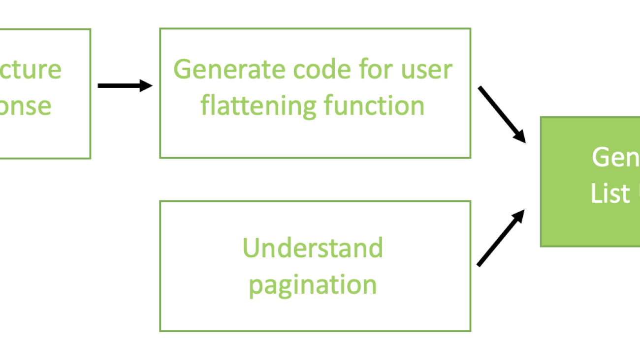


 Xiong Zhou is a Senior Applied Scientist at AWS. He leads the science team for Amazon SageMaker geospatial capabilities. His current area of research includes LLM evaluation and data generation. In his spare time, he enjoys running, playing basketball and spending time with his family.
 Anirudh Viswanathan is a Sr Product Manager, Technical – External Services with the SageMaker geospatial ML team. He holds a Masters in Robotics from Carnegie Mellon University, an MBA from the Wharton School of Business, and is named inventor on over 40 patents. He enjoys long-distance running, visiting art galleries and Broadway shows.
 Janosch Woschitz is a Senior Solutions Architect at AWS, specializing in AI/ML. With over 15 years of experience, he supports customers globally in leveraging AI and ML for innovative solutions and building ML platforms on AWS. His expertise spans machine learning, data engineering, and scalable distributed systems, augmented by a strong background in software engineering and industry expertise in domains such as autonomous driving.
 Li Erran Li is the applied science manager at humain-in-the-loop services, AWS AI, Amazon. His research interests are 3D deep learning, and vision and language representation learning. Previously he was a senior scientist at Alexa AI, the head of machine learning at Scale AI and the chief scientist at Pony.ai. Before that, he was with the perception team at Uber ATG and the machine learning platform team at Uber working on machine learning for autonomous driving, machine learning systems and strategic initiatives of AI. He started his career at Bell Labs and was adjunct professor at Columbia University. He co-taught tutorials at ICML’17 and ICCV’19, and co-organized several workshops at NeurIPS, ICML, CVPR, ICCV on machine learning for autonomous driving, 3D vision and robotics, machine learning systems and adversarial machine learning. He has a PhD in computer science at Cornell University. He is an ACM Fellow and IEEE Fellow.
 Amit Modi is the product leader for SageMaker MLOps, ML Governance, and Responsible AI at AWS. With over a decade of B2B experience, he builds scalable products and teams that drive innovation and deliver value to customers globally.
 Kris Efland is a visionary technology leader with a successful track record in driving product innovation and growth for over 20 years. Kris has helped create new products including consumer electronics and enterprise software across many industries, at both startups and large companies. In his current role at Amazon Web Services (AWS), Kris leads the Geospatial AI/ML category. He works at the forefront of Amazon’s fastest-growing ML service, Amazon SageMaker, which serves over 100,000 customers worldwide. He recently led the launch of Amazon SageMaker’s new geospatial capabilities, a powerful set of tools that allow data scientists and machine learning engineers to build, train, and deploy ML models using satellite imagery, maps, and location data. Before joining AWS, Kris was the Head of Autonomous Vehicle (AV) Tools and AV Maps for Lyft, where he led the company’s autonomous mapping efforts and toolchain used to build and operate Lyft’s fleet of autonomous vehicles. He also served as the Director of Engineering at HERE Technologies and Nokia and has co-founded several startups..


 Étienne Brouillard is an AWS AI Principal Architect at Intact Financial Corporation, Canada’s largest provider of property and casualty insurance.
 Ami Dani is a Senior Technical Program Manager at AWS focusing on AI/ML services. During her career, she has focused on delivering transformative software development projects for the federal government and large companies in industries as diverse as advertising, entertainment, and finance. Ami has experience driving business growth, implementing innovative training programs and successfully managing complex, high-impact projects.
 Prabir Sekhri is a Senior Solutions Architect at AWS in the enterprise financial services sector. During his career, he has focused on digital transformation projects within large companies in industries as diverse as finance, multimedia, telecommunications as well as the energy and gas sectors. His background includes DevOps, security, and designing and architecting enterprise storage solutions. Besides technology, Prabir has always been passionate about playing music. He leads a jazz ensemble in Montreal as a pianist, composer and arranger.


 Ebbey Thomas is a Senior Cloud Architect at AWS, with a strong focus on leveraging generative AI to enhance cloud infrastructure automation and accelerate migrations. In his role at AWS Professional Services, Ebbey designs and implements solutions that improve cloud adoption speed and efficiency while ensuring secure and scalable operations for AWS users. He is known for solving complex cloud challenges and driving tangible results for clients. Ebbey holds a BS in Computer Engineering and an MS in Information Systems from Syracuse University.
 Shiva Vaidyanathan is a Principal Cloud Architect at AWS. He provides technical guidance, design and lead implementation projects to customers ensuring their success on AWS. He works towards making cloud networking simpler for everyone. Prior to joining AWS, he has worked on several NSF funded research initiatives on performing secure computing in public cloud infrastructures. He holds a MS in Computer Science from Rutgers University and a MS in Electrical Engineering from New York University.
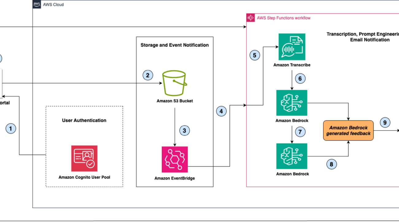


 Nehal Sangoi is a Sr. Technical Account Manager at Amazon Web Services. She provides strategic technical guidance to help independent software vendors plan and build solutions using AWS best practices. Connect with Nehal on
  Akshay Singhal is a Sr. Technical Account Manager at Amazon Web Services supporting Enterprise Support customers focusing on the Security ISV segment. He provides technical guidance for customers to implement AWS solutions, with expertise spanning serverless architectures and cost optimization. Outside of work, Akshay enjoys traveling, Formula 1, making short movies, and exploring new cuisines. Connect with him on


 Bar Fingerman is the Head of AI/ML Engineering at Bria. He leads the development and optimization of core infrastructure, enabling the company to scale cutting-edge generative AI technologies. With a focus on designing high-performance supercomputers for large-scale AI training, Bar leads the engineering group in deploying, managing, and securing scalable AI/ML cloud solutions. He works closely with leadership and cross-functional teams to align business goals while driving innovation and cost-efficiency.
 Supriya Puragundla is a Senior Solutions Architect at AWS. She has over 15 years of IT experience in software development, design, and architecture. She helps key customer accounts on their data, generative AI, and AI/ML journeys. She is passionate about data-driven AI and the area of depth in ML and generative AI.
 Rodrigo Merino is a Generative AI Solutions Architect Manager at AWS. With over a decade of experience deploying emerging technologies, ranging from generative AI to IoT, Rodrigo guides customers across various industries to accelerate their AI/ML and generative AI journeys. He specializes in helping organizations train and build models on AWS, as well as operationalize end-to-end ML solutions. Rodrigo’s expertise lies in bridging the gap between cutting-edge technology and practical business applications, enabling companies to harness the full potential of AI and drive innovation in their respective fields.
 Eliad Maimon is a Senior Startup Solutions Architect at AWS, focusing on generative AI startups. He helps startups accelerate and scale their AI/ML journeys by guiding them through deep-learning model training and deployment on AWS. With a passion for AI and entrepreneurship, Eliad is committed to driving innovation and growth in the startup ecosystem.