The AWS Generative AI Innovation Center (GenAIIC) is a team of AWS science and strategy experts who have deep knowledge of generative AI. They help AWS customers jumpstart their generative AI journey by building proofs of concept that use generative AI to bring business value. Since the inception of AWS GenAIIC in May 2023, we have witnessed high customer demand for chatbots that can extract information and generate insights from massive and often heterogeneous knowledge bases. Such use cases, which augment a large language model’s (LLM) knowledge with external data sources, are known as Retrieval-Augmented Generation (RAG).
This two-part series shares the insights gained by AWS GenAIIC from direct experience building RAG solutions across a wide range of industries. You can use this as a practical guide to building better RAG solutions.
In this first post, we focus on the basics of RAG architecture and how to optimize text-only RAG. The second post outlines how to work with multiple data formats such as structured data (tables, databases) and images.
Anatomy of RAG
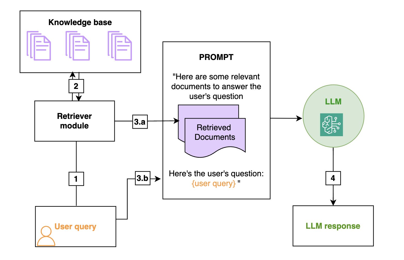
RAG is an efficient way to provide an FM with additional knowledge by using external data sources and is depicted in the following diagram:
- Retrieval: Based on a user’s question (1), relevant information is retrieved from a knowledge base (2) (for example, an OpenSearch index).
- Augmentation: The retrieved information is added to the FM prompt (3.a) to augment its knowledge, along with the user query (3.b).
- Generation: The FM generates an answer (4) by using the information provided in the prompt.
The following is a general diagram of a RAG workflow. From left to right are the retrieval, the augmentation, and the generation. In practice, the knowledge base is often a vector store.
A deeper dive in the retriever
In a RAG architecture, the FM will base its answer on the information provided by the retriever. Therefore, a RAG is only as good as its retriever, and many of the tips that we share in our practical guide are about how to optimize the retriever. But what is a retriever exactly? Broadly speaking, a retriever is a module that takes a query as input and outputs relevant documents from one or more knowledge sources relevant to that query.
Document ingestion
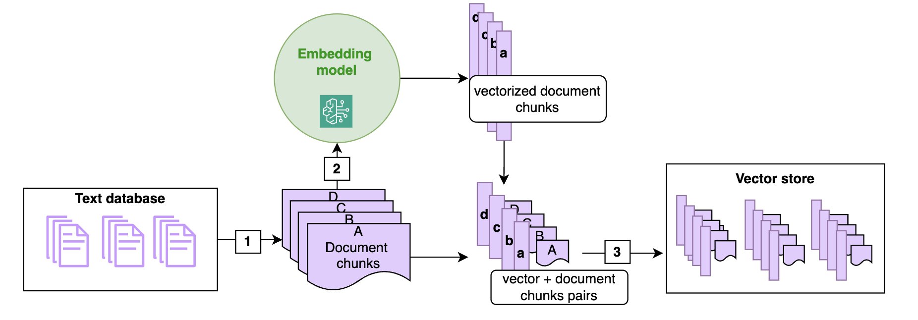
In a RAG architecture, documents are often stored in a vector store. As shown in the following diagram, vector stores are populated by chunking the documents into manageable pieces (1) (if a document is short enough, chunking might not be required) and transforming each chunk of the document into a high-dimensional vector using a vector embedding (2), such as the Amazon Titan embeddings model. These embeddings have the characteristic that two chunks of texts that are semantically close have vector representations that are also close in that embedding (in the sense of the cosine or Euclidean distance).
The following diagram illustrates the ingestion of text documents in the vector store using an embedding model. Note that the vectors are stored alongside the corresponding text chunk (3), so that at retrieval time, when you identify the chunks closest to the query, you can return the text chunk to be passed to the FM prompt.
Semantic search
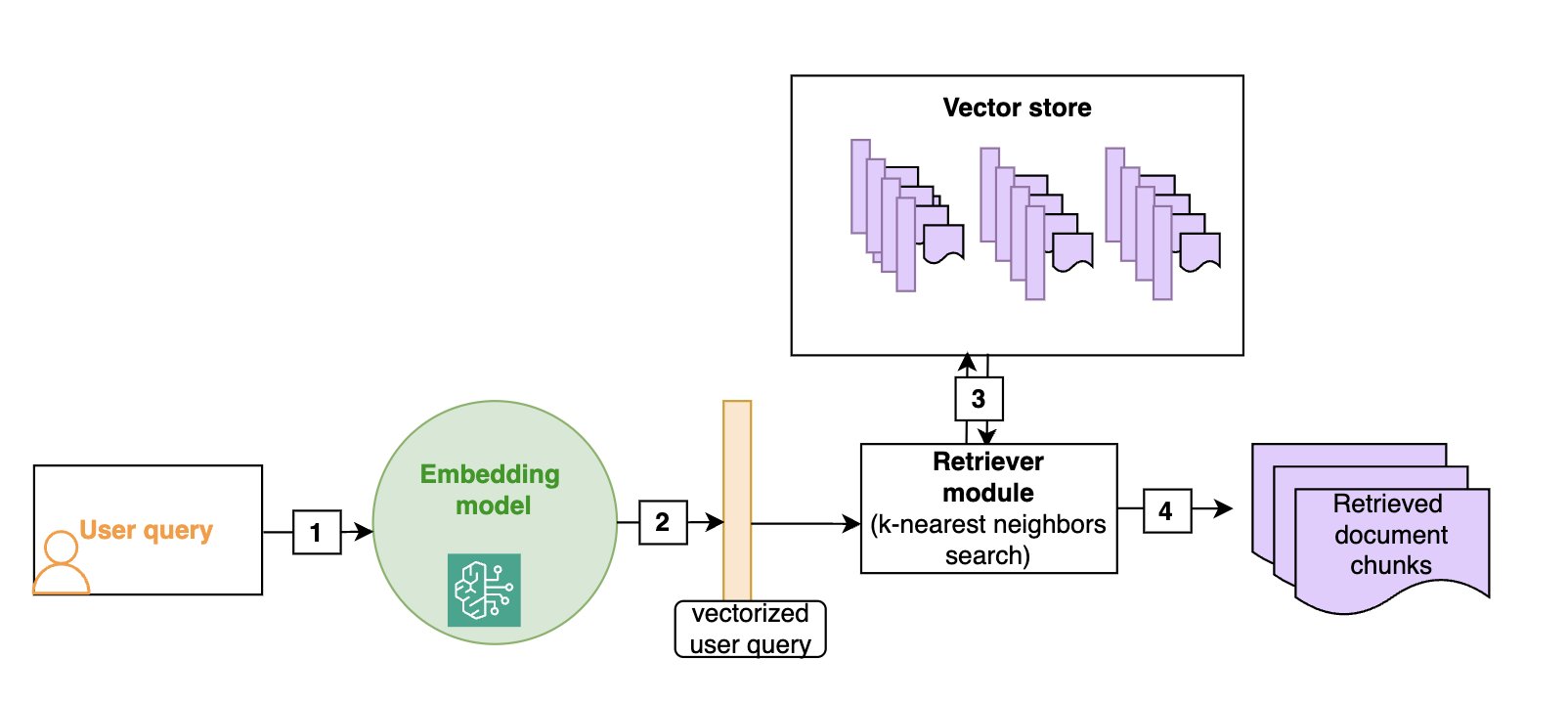
Vector stores allow for efficient semantic search: as shown in the following diagram, given a user query (1), we vectorize it (2) (using the same embedding as the one that was used to build the vector store) and then look for the nearest vectors in the vector store (3), which will correspond to the document chunks that are semantically closest to the initial query (4). Although vector stores and semantic search have become the default in RAG architectures, more traditional keyword-based search is still valuable, especially when searching for domain-specific words (such as technical jargon) or names. Hybrid search is a way to use both semantic search and keywords to rank a document, and we will give more details on this technique in the section on advanced RAG techniques.
The following diagram illustrates the retrieval of text documents that are semantically close to the user query. You must use the same embedding model at ingestion time and at search time.
Implementation on AWS
A RAG chatbot can be set up in a matter of minutes using Amazon Bedrock Knowledge Bases. The knowledge base can be linked to an Amazon Simple Storage Service (Amazon S3) bucket and will automatically chunk and index the documents it contains in an OpenSearch index, which will act as the vector store. The retrieve_and_generate API does both the retrieval and a call to an FM (Amazon Titan or Anthropic’s Claude family of models on Amazon Bedrock), for a fully managed solution. The retrieve API only implements the retrieval component and allows for a more custom approach downstream, such as document post processing before calling the FM separately.
In this blog post, we will provide tips and code to optimize a fully custom RAG solution with the following components:
- An OpenSearch Serverless vector search collection as the vector store
- Custom chunking and ingestion functions to ingest the documents in the OpenSearch index
- A custom retrieval function that takes a user query as an input and outputs the relevant documents from the OpenSearch index
- FM calls to your model of choice on Amazon Bedrock to generate the final answer.
In this post, we focus on a custom solution to help readers understand the inner workings of RAG. Most of the tips we provide can be adapted to work with Amazon Bedrock Knowledge Bases, and we will point this out in the relevant sections.
Overview of RAG use cases
While working with customers on their generative AI journey, we encountered a variety of use cases that fit within the RAG paradigm. In traditional RAG use cases, the chatbot relies on a database of text documents (.doc, .pdf, or .txt). In part 2 of this post, we will discuss how to extend this capability to images and structured data. For now, we’ll focus on a typical RAG workflow: the input is a user question, and the output is the answer to that question, derived from the relevant text chunks or documents retrieved from the database. Use cases include the following:
- Customer service– This can include the following:
- Internal– Live agents use an internal chatbot to help them answer customer questions.
- External– Customers directly chat with a generative AI chatbot.
- Hybrid– The model generates smart replies for live agents that they can edit before sending to customers.
- Employee training and resources– In this use case, chatbots can use employee training manuals, HR resources, and IT service documents to help employees onboard faster or find the information they need to troubleshoot internal issues.
- Industrial maintenance– Maintenance manuals for complex machines can have several hundred pages. Building a RAG solution around these manuals helps maintenance technicians find relevant information faster. Note that maintenance manuals often have images and schemas, which could put them in a multimodal bucket.
- Product information search– Field specialists need to identify relevant products for a given use case, or conversely find the right technical information about a given product.
- Retrieving and summarizing financial news– Analysts need the most up-to-date information on markets and the economy and rely on large databases of news or commentary articles. A RAG solution is a way to efficiently retrieve and summarize the relevant information on a given topic.
In the following sections, we will give tips that you can use to optimize each aspect of the RAG pipeline (ingestion, retrieval, and answer generation) depending on the underlying use case and data format. To verify that the modifications improve the solution, you first need to be able to assess the performance of the RAG solution.
Evaluating a RAG solution
Contrary to traditional machine learning (ML) models, for which evaluation metrics are well defined and straightforward to compute, evaluating a RAG framework is still an open problem. First, collecting ground truth (information known to be correct) for the retrieval component and the generation component is time consuming and requires human intervention. Secondly, even with several question-and-answer pairs available, it’s difficult to automatically evaluate if the RAG answer is close enough to the human answer.
In our experience, when a RAG system performs poorly, we found the retrieval part to almost always be the culprit. Large pre-trained models such as Anthropic’s Claude model will generate high-quality answers if provided with the right information, and we notice two main failure modes:
- The relevant information isn’t present in the retrieved documents: In this case, the FM can try to make up an answer or use its own knowledge to answer. Adding guardrails against such behavior is essential.
- Relevant information is buried within an excessive amount of irrelevant data: When the scope of the retriever is too broad, the FM can get confused and start mixing up multiple data sources, resulting in a wrong answer. More advanced models such as Anthropic’s Claude Sonnet 3.5 and Opus are reported to be more robust against such behavior, but this is still a risk to be aware of.
To evaluate the quality of the retriever, you can use the following traditional retrieval metrics:
- Top-k accuracy: Measures whether at least one relevant document is found within the top k retrieved documents.
- Mean Reciprocal Rank (MRR)– This metric considers the ranking of the retrieved documents. It’s calculated as the average of the reciprocal ranks (RR) for each query. The RR is the inverse of the rank position of the first relevant document. For example, if the first relevant document is in third position, the RR is 1/3. A higher MRR indicates that the retriever can rank the most relevant documents higher.
- Recall– This metric measures the ability of the retriever to retrieve relevant documents from the corpus. It’s calculated as the number of relevant documents that are successfully retrieved over the total number of relevant documents. Higher recall indicates that the retriever can find most of the relevant information.
- Precision– This metric measures the ability of the retriever to retrieve only relevant documents and avoid irrelevant ones. It’s calculated by the number of relevant documents successfully retrieved over the total number of documents retrieved. Higher precision indicates that the retriever isn’t retrieving too many irrelevant documents.
Note that if the documents are chunked, the metrics must be computed at the chunk level. This means the ground truth to evaluate a retriever is pairs of question and list of relevant document chunks. In many cases, there is only one chunk that contains the answer to the question, so the ground truth becomes question and relevant document chunk.
To evaluate the quality of the generated response, two main options are:
- Evaluation by subject matter experts: this provides the highest reliability in terms of evaluation but can’t scale to a large number of questions and slows down iterations on the RAG solution.
- Evaluation by FM (also called LLM-as-a-judge):
- With a human-created starting point: Provide the FM with a set of ground truth question-and-answer pairs and ask the FM to evaluate the quality of the generated answer by comparing it to the ground truth one.
- With an FM-generated ground truth: Use an FM to generate question-and-answer pairs for given chunks, and then use this as a ground truth, before resorting to an FM to compare RAG answers to that ground truth.
We recommend that you use an FM for evaluations to iterate faster on improving the RAG solution, but to use subject-matter experts (or at least human evaluation) to provide a final assessment of the generated answers before deploying the solution.
A growing number of libraries offer automated evaluation frameworks that rely on additional FMs to create a ground truth and evaluate the relevance of the retrieved documents as well as the quality of the response:
- Ragas– This framework offers FM-based metrics previously described, such as context recall, context precision, answer faithfulness, and answer relevancy. It needs to be adapted to Anthropic’s Claude models because of its heavy dependence on specific prompts.
- LlamaIndex– This framework provides multiple modules to independently evaluate the retrieval and generation components of a RAG system. It also integrates with other tools such as Ragas and DeepEval. It contains modules to create ground truth (query-and-context pairs and question-and-answer pairs) using an FM, which alleviates the use of time-consuming human collection of ground truth.
- RefChecker– This is an Amazon Science library focused on fine-grained hallucination detection.
Troubleshooting RAG
Evaluation metrics give an overall picture of the performance of retrieval and generation, but they don’t help diagnose issues. Diving deeper into poor responses can help you understand what’s causing them and what you can do to alleviate the issue. You can diagnose the issue by looking at evaluation metrics and also by having a human evaluator take a closer look at both the LLM answer and the retrieved documents.
The following is a brief overview of issues and potential fixes. We will describe each of the techniques in more detail, including real-world use cases and code examples, in the next section.
- The relevant chunk wasn’t retrieved (retriever has low top k accuracy and low recall or spotted by human evaluation):
- Try increasing the number of documents retrieved by the nearest neighbor search and re-ranking the results to cut back on the number of chunks after retrieval.
- Try hybrid search. Using keywords in combination with semantic search (known as hybrid search) might help, especially if the queries contain names or domain-specific jargon.
- Try query rewriting. Having an FM detect the intent or rewrite the query can help create a query that’s better suited for the retriever. For instance, a user query such as “What information do you have in the knowledge base about the economic outlook in China?” contains a lot of context that isn’t relevant to the search and would be more efficient if rewritten as “economic outlook in China” for search purposes.
- Too many chunks were retrieved (retriever has low precision or spotted by human evaluation):
- Try using keyword matching to restrict the search results. For example, if you’re looking for information about a specific entity or property in your knowledge base, only retrieve documents that explicitly mention them.
- Try metadata filtering in your OpenSearch index. For example, if you’re looking for information in news articles, try using the date field to filter only the most recent results.
- Try using query rewriting to get the right metadata filtering. This advanced technique uses the FM to rewrite the user query as a more structured query, allowing you to make the most of OpenSearch filters. For example, if you’re looking for the specifications of a specific product in your database, the FM can extract the product name from the query, and you can then use the product name field to filter out the product name.
- Try using reranking to cut down on the number of chunks passed to the FM.
- A relevant chunk was retrieved, but it’s missing some context (can only be assessed by human evaluation):
- Try changing the chunking strategy. Keep in mind that small chunks are good for precise questions, while large chunks are better for questions that require a broad context:
- Try increasing the chunk size and overlap as a first step.
- Try using section-based chunking. If you have structured documents, use sections delimiters to cut your documents into chunks to have more coherent chunks. Be aware that you might lose some of the more fine-grained context if your chunks are larger.
- Try small-to-large retrievers. If you want to keep the fine-grained details of small chunks but make sure you retrieve all the relevant context, small-to-large retrievers will retrieve your chunk along with the previous and next ones.
- If none of the above help:
- Consider training a custom embedding.
- The retriever isn’t at fault, the problem is with FM generation (evaluated by a human or LLM):
- Try prompt engineering to mitigate hallucinations.
- Try prompting the FM to use quotes in its answers, to allow for manual fact checking.
- Try using another FM to evaluate or correct the answer.
A practical guide to improving the retriever
Note that not all the techniques that follow need to be implemented together to optimize your retriever—some might even have opposite effects. Use the preceding troubleshooting guide to get a shortlist of what might work, then look at the examples in the corresponding sections that follow to assess if the method can be beneficial to your retriever.
Hybrid search
Example use case: A large manufacturer built a RAG chatbot to retrieve product specifications. These documents contain technical terms and product names. Consider the following example queries:
query_1 = "What is the viscosity of product XYZ?"
query_2 = "How viscous is XYZ?"
The queries are equivalent and need to be answered with the same document. The keyword component will make sure that you’re boosting documents mentioning the name of the product, XYZ while the semantic component will make sure that documents containing viscosity get a high score, even when the query contains the word viscous.
Combining vector search with keyword search can effectively handle domain-specific terms, abbreviations, and product names that embedding models might struggle with. Practically, this can be achieved in OpenSearch by combining a k-nearest neighbors (k-NN) query with keyword matching. The weights for the semantic search compared to keyword search can be adjusted. See the following example code:
vector_embedding = compute_embedding(query)
size = 10
semantic_weight = 10
keyword_weight = 1
search_query = {"size":size, "query": { "bool": { "should":[] , "must":[] } } }
    # semantic search
    search_query['query']['bool']['should'].append(
            {"function_score":
             { "query":
              {"knn":
               {"vector_field":
                {"vector": vector_embedding,
                "k": 10 # The number of nearest neighbors to retrieve
                }}},
              "weight": semantic_weight } })

    # keyword search
    search_query['query']['bool']['should'].append({
             "function_score":
            { "query":
             {"match":
             # This will increase the score of chunks that match the words in the query
              {"chunk_text":  query}
              },
             "weight": keyword_weight } })
Amazon Bedrock Knowledge Bases also supports hybrid search, but you can’t adjust the weights for semantic compared to keyword search.
Adding metadata information to text chunks
Example use case: Using the same example of a RAG chatbot for product specifications, consider product specifications that are several pages long and where the product name is only present in the header of the document. When ingesting the document into the knowledge base, it’s chunked into smaller pieces for the embedding model, and the product name only appears in the first chunk, which contains the header. See the following example:
# Note: the following document was generated by Anthropic’s Claude Sonnet
# and does not contain information about a real product

document_name = "Chemical Properties for Product XYZ"

chunk_1 = """
Product Description:
XYZ is a multi-purpose cleaning solution designed for industrial and commercial use.
It is a concentrated liquid formulation containing anionic and non-ionic surfactants,
solvents, and alkaline builders.

Chemical Composition:
- Water (CAS No. 7732-18-5): 60-80%
- 2-Butoxyethanol (CAS No. 111-76-2): 5-10%
- Sodium Hydroxide (CAS No. 1310-73-2): 2-5%
- Ethoxylated Alcohols (CAS No. 68439-46-3): 1-3%
- Sodium Metasilicate (CAS No. 6834-92-0): 1-3%
- Fragrance (Proprietary Mixture): <1%
"""

# chunk 2 below doesn't contain any mention of "XYZ"
chunk_2 = """
Physical Properties:
- Appearance: Clear, yellow liquid
- Odor: Mild, citrus fragrance
- pH (concentrate): 12.5 - 13.5
- Specific Gravity: 1.05 - 1.10
- Solubility in Water: Complete
- VOC Content: <10%

Shelf-life:
When stored in its original, unopened container at temperatures between 15°C and 25°C,
 the product has a shelf life of 24 months from the date of manufacture.
Once opened, the shelf life is reduced due to potential contamination and exposure to
 air. It is recommended to use the product within 6 months after opening the container.
"""
The chunk containing information about the shelf life of XYZ doesn’t contain any mention of the product name, so retrieving the right chunk when searching for shelf life of XYZ among dozens of other documents mentioning the shelf life of various products isn’t possible. A solution is to prepend the document name or title to each chunk. This way, when performing a hybrid search about the shelf life of product XYZ, the relevant chunk is more likely to be retrieved.
# append the document name to the chunks to improve context,
# now chunk 2 will contain the product name

chunk_1 = document_name + chunk_1
chunk_2 = document_name + chunk_2
This is one way to use document metadata to improve search results, which can be sufficient in some cases. Later, we discuss how you can use metadata to filter the OpenSearch index.
Small-to-large chunk retrieval
Example use case: A customer built a chatbot to help their agents better serve customers. When the agent tries to help a customer troubleshoot their internet access, he might search for How to troubleshoot internet access? You can see a document where the instructions are split between two chunks in the following example. The retriever will most likely return the first chunk but might miss the second chunk when using hybrid search. Prepending the document title might not help in this example.
document_title = "Resolving network issues"

chunk_1 = """
[....]

# Troubleshooting internet access:

1. Check your physical connections:
   - Ensure that the Ethernet cable (if using a wired connection) is securely
   plugged into both your computer and the modem/router.
   - If using a wireless connection, check that your device's Wi-Fi is turned
   on and connected to the correct network.

2. Restart your devices:
   - Reboot your computer, laptop, or mobile device.
   - Power cycle your modem and router by unplugging them from the power source,
   waiting for a minute, and then plugging them back in.

"""

chunk_2 = """
3. Check for network outages:
   - Contact your internet service provider (ISP) to inquire about any known
   outages or service disruptions in your area.
   - Visit your ISP's website or check their social media channels for updates on
   service status.

4. Check for interference:
   - If using a wireless connection, try moving your device closer to the router or access point.
   - Identify and eliminate potential sources of interference, such as microwaves, cordless phones, or other wireless devices operating on the same frequency.

# Router configuration

[....]
"""
To mitigate this issue, the first thing to try is to slightly increase the chunk size and overlap, reducing the likelihood of improper segmentation, but this requires trial and error to find the right parameters. A more effective solution is to employ a small-to-large chunk retrieval strategy. After retrieving the most relevant chunks through semantic or hybrid search (chunk_1 in the preceding example), adjacent chunks (chunk_2) are retrieved, merged with the initial chunks and provided to the FM for a broader context. You can even pass the full document text if the size is reasonable.
This method requires an additional OpenSearch field in the index to keep track of the chunk number and document name at ingest time, so that you can use those to retrieve the neighboring chunks after retrieving the most relevant chunk. See the following code example.
document_name = doc['document_name']
current_chunk = doc['current_chunk']

query = {
    "query": {
        "bool": {
            "must": [
                {
                    "match": {
                        "document_name": document_name
                    }
                }
            ],
            "should": [
                {"term": {"chunk_number": current_chunk - 1}},
                {"term": {"chunk_number": current_chunk + 1}}
            ],
            "minimum_should_match": 1
        }
    }
}
A more general approach is to do hierarchical chunking, in which each small (child) chunk is linked to a larger (parent) chunk. At retrieval time, you retrieve the child chunks, but then replace them with the parent chunks before sending the chunks to the FM.
Amazon Bedrock Knowledge Bases can perform hierarchical chunking.
Section-based chunking
Example use case: A financial news provider wants to build a chatbot to retrieve and summarize commentary articles about certain geographic regions, industries, or financial products. The questions require a broad context, such as What is the outlook for electric vehicles in China? Answering that question requires access to the entire section on electric vehicles in the “Chinese Auto Industry Outlook” commentary article. Compare that to other question and answer use cases that require small chunks to answer a question (such as our example about searching for product specifications).
Example use case: Section based chunking also works well for how-to-guides (such as the preceding internet troubleshooting example) or industrial maintenance use cases where the user needs to follow step-by-step instructions and having truncated content would have a negative impact.
Using the structure of the text document to determine where to split it is an efficient way to create chunks that are coherent and contain all relevant context. If the document is in HTML or Markdown format, you can use the section delimiters to determine the chunks (see Langchain Markdown Splitter or HTML Splitter). If the documents are in PDF format, the Textractor library provides a wrapper around Amazon Textract that uses the Layout feature to convert a PDF document to Markdown or HTML.
Note that section-based chunking will create chunks with varying size, and they might not fit the context window of Cohere Embed, which is limited to 500 tokens. Amazon Titan Text Embeddings are better suited to section-based chunking because of their context window of 8,192 tokens.
To implement section based chunking in Amazon Bedrock Knowledge Bases, you can use an AWS Lambda function to run a custom transformation. Amazon Bedrock Knowledge Bases also has a feature to create semantically coherent chunks, called semantic chunking. Instead of using the sections of the documents to determine the chunks, it uses embedding distance to create meaningful clusters of sentences.
Rewriting the user query
Query rewriting is a powerful technique that can benefit a variety of use cases.
Example use case: A RAG chatbot that’s built for a food manufacturer allows customers to ask questions about products, such as ingredients, shelf-life, and allergens. Consider the following example query:
query = """"
Can you list all the ingredients in the nuts and seeds granola?
Put the allergens in all caps.
"""
Query rewriting can help with two things:
- It can rewrite the query just for search purposes, without information about formatting that might distract the retriever.
- It can extract a list of keywords to use for hybrid search.
- It can extract the product name, which can be used as a filter in the OpenSearch index to refine search results (more details in the next section).
In the following code, we prompt the FM to rewrite the query and extract keywords and the product name. To avoid introducing too much latency with query rewriting, we suggest using a smaller model like Anthropic’s Claude Haiku and provide an example of a reformatted query to boost the performance.
import json

query_rewriting_prompt = """
Rewrite the query as a json with the following keys:
- rewritten_query: a better version of the user's query that will be used to compute
an embedding and do semantic search
- keywords: a list of keywords that correspond to the query, to be used in a
search engine, it should not contain the product name.
- product_name: if the query is a about a specific product, give the name here,
 otherwise say None.

<example>
H: what are the ingedients in the savory trail mix?
A: {{
  "rewritten_query": "ingredients savory trail mix",
  "keywords": ["ingredients"],
  "product_name": "savory trail mix"
}}
</example>

<query>
{query}
</query>

Only output the json, nothing else.
"""

def rewrite_query(query):
    response = call_FM(query_rewriting_prompt.format(query=query))
    print(response)
    json_query = json.loads(response)
    return json_query

rewrite_query(query)
The code output will be the following json:
{
"rewritten_query":"ingredients nuts and seeds granola allergens",
"keywords": ["ingredients", "allergens"],
"product_name": "nuts and seeds granola"
}
Amazon Bedrock Knowledge Bases now supports query rewriting. See this tutorial.
Metadata filtering
Example use case: Let’s continue with the previous example, where a customer asks “Can you list all the ingredients in the nuts and seeds granola? Put the allergens in bold and all caps.” Rewriting the query allowed you to remove superfluous information about the formatting and improve the results of hybrid search. However, there might be dozens of products that are either granola, or nuts, or granola with nuts.
If you enforce an OpenSearch filter to match exactly the product name, the retriever will return only the product information for nuts and seeds granola instead of the k-nearest documents when using hybrid search. This will reduce the number of tokens in the prompt and will both improve latency of the RAG chatbot and diminish the risk of hallucinations because of information overload.
This scenario requires setting up the OpenSearch index with metadata. Note that if your documents don’t come with metadata attached, you can use an FM at ingest time to extract metadata from the documents (for example, title, date, and author).
oss = get_opensearch_serverless_client()
request = {
"product_info": product_info, # full text for the product information
"vector_field_product":embed_query_titan(product_info), # embedding for product information
"product_name": product_name,
"date": date, # optional field, can allow to sort by most recent
"_op_type": "index",
"source": file_key # this is the s3 location, you can replace this with a URL
}
oss.index(index = index_name, body = request)
The following is an example of combining hybrid search, query rewriting, and filtering on the product_name field. Note that for the product name, we use a match_phrase clause to make sure that if the product name contains several words, the product name is matched in full; that is, if the product you’re looking for is “nuts and seeds granola”, you don’t want to match all product names that contain “nuts”, “seeds”, or “granola”.
query = """
Can you list all the ingredients in the nuts and seeds granola?
Put the allergens in bold and all caps.
"""
# using the rewrite_query function from the previous section
json_query = rewrite_query(query)

# get the product name and keywords from the json query
product_name = json_query["product_name"]
keywords = json_query["keywords"]

# compute the vector embedding of the rewritten query
vector_embedding = compute_embedding(json_query["rewritten_query"])

#initialize search query dictionary
search_query = {"size":10, "query": { "bool": { "should":[] , "must":[] } } }
# add must with match_phrase clause to filter on product name
search_query['query']['bool']['should'].append(
    {"match_phrase": {
            "product_name": product_name # Extracted product name must match product name field
        }
        }

# semantic search
search_query['query']['bool']['should'].append(
        {"function_score":
            { "query":
            {"knn":
            {"vector_field_product":
            {"vector": vector_embedding,
            "k": 10 # The number of nearest neighbors to retrieve
            }}},
            "weight": semantic_weight } })

# keyword search
search_query['query']['bool']['should'].append(
{"function_score":
        { "query":
            {"match":
            # This will increase the score of chunks that match the words in the query
            {"product_info":  query}
            },
            "weight": keyword_weight } })
Amazon Bedrock Knowledge Bases recently introduced the ability to use metadata. See Amazon Bedrock Knowledge Bases now supports metadata filtering to improve retrieval accuracy for details on the implementation.
Training custom embeddings
Training custom embeddings is a more expensive and time-consuming way to improve a retriever, so it shouldn’t be the first thing to try to improve your RAG. However, if the performance of the retriever is still not satisfactory after trying the tips already mentioned, then training a custom embedding can boost its performance. Amazon Titan Text Embeddings models aren’t currently available for fine tuning, but the FlagEmbedding library on Hugging Face provides a way to fine-tune BAAI embeddings, which are available in several sizes and rank highly in the Hugging Face embedding leaderboard. Fine-tuning requires the following steps:
- Gather positive question-and-document pairs. You can do this manually or by using an FM prompted to generate questions based on the document.
- Gather negative question-and-document pairs. It’s important to focus on documents that might be considered relevant by the pre-trained model but are not. This process is called hard negative mining.
- Feed those pairs to the
FlagEmbedding training module for fine-tuning as a JSON:
{"query": str, "pos": List[str], "neg":List[str]}
where query is the query, pos is a list of positive texts, and neg is a list of negative texts.
- Combine the fine-tuned model with a pre-trained model using to avoid over-fitting on the fine-tuning dataset.
- Deploy the final model for inference, for example on Amazon SageMaker, and evaluate it on sample questions.
Improving reliability of generated responses
Even with an optimized retriever, hallucinations can still occur. Prompt engineering is the best way to help prevent hallucinations in RAG. Additionally, asking the FM to generate quotations used in the answer can further reduce hallucinations and empower the user to verify the information sources.
Prompt engineering guardrails
Example use case: We built a chatbot that analyzes scouting reports for a professional sports franchise. The user might input What are the strengths of Player X? Without guardrails in the prompt, the FM might try to fill the gaps in the provided documents by using its own knowledge of Player X (if he’s a well-known player) or worse, make up information by combining knowledge it has about other players.
The FM’s training knowledge can sometimes get in the way of RAG answers. Basic prompting techniques can help mitigate hallucinations:
- Instruct the FM to only use information available in the documents to answer the question.
Only use the information available in the documents to answer the question
- Giving the FM the option to say when it doesn’t have the answer.
If you can’t answer the question based on the documents provided, say you don’t know.
Asking the FM to output quotes
Another approach to make answers more reliable is to output supporting quotations. This has two benefits:
- It allows the FM to generate its response by first outputting the relevant quotations, and then using them to generate its answer.
- The presence of the quotation in the cited document can be checked programmatically, and the user can be warned if the quotation wasn’t found in the text. They can also look in the referenced document to get more context about the quotation.
In the following example, we prompt the FM to output quotations in <quote> tags. The quotations are nicely formatted as a JSON, with the source document name. Note how we put each document in its own <doc_i> tag in the prompt, so that the FM can reference it.
# Note: The scouting reports for Player A and Player B used in the example below
# were generated by Anthropic’s Claude Sonnet 3.
quotes_tags_prompt = """
You are an Ai assistant chatbot designed to answer questions about your team's baseballe scouting reports.

Here are some reports about players that you can use to answer the question:

<doc_0>
{doc_0}
</doc_0>

<doc_1>
{doc_1}
</doc_1>

<instructions>
- In <scratchpad> tags, you should put the document names and quotes from these documents
 that help you answer this question.
 You must format this as one or more jsons format with 'document_name' and 'quote' as keys.
- Then put your answer in <answer> tags.
 If you refer to documents in your answer, make sure you are using the corresponding tag
 e.g. in doc_0, in doc_3 etc.
- If you can't answer the question because there is not enough information in the reports say
 "I can't answer this based on the provided reports."
</instructions>

<question>
{question}
</question>
"""
Below is the FM response to the question "What are the weaknesses of each player?":
"""
<scratchpad>
[
{
"document_name": "doc_0",
"quote": "The main concern with Player A is his approach at the plate. He can be overly aggressive at times and will chase pitches out of the zone. Improving his plate discipline and pitch recognition will be key to him reaching his full offensive potential."
},
{
"document_name": "doc_1",
"quote": "The main area of focus for Player B's development will be improving his plate discipline and pitch recognition. He can be overly aggressive at times, leading to a high strikeout rate and a lower on-base percentage than his hit tool would suggest."
}
]
</scratchpad>
<answer>
The main weaknesses of the players are:
For Player A:
- Overly aggressive approach at the plate, chasing pitches out of the zone
- Needs to improve plate discipline and pitch recognition to reach full offensive potential
For Player B:
- Can be overly aggressive at the plate, leading to high strikeout rate and lower on-base percentage
- Needs to improve plate discipline and pitch recognition
</answer>
"""
One drawback of generating quotations outside of the answer is that the FM tends to only select one or two short quotations per document. This doesn’t make it a great choice when you’re asking complex questions that need to pull a lot of information from diverse documents. It also leads to creating more output tokens that are eventually hidden from the user, which can significantly degrade the latency of the RAG if the quotations are too long.
Generating an answer with inline quotations
Continuing the example of the chatbot to analyze scouting reports, the user might want to summarize reports about a player from several scouts. A single player can have over a dozen scouting reports that the FM could use in its summary, and the previous method outputs only a small number of quotations as justification. One alternative is to ask the FM to embed quotations directly in the answer, by using quotation marks and inline citations.
# Note: The scouting reports for Player A used in the example below
# were generated by Anthropic’s Claude Sonnet 3.

quotes_in_text_prompt = """
You are an Ai assistant chatbot designed to answer questions about your team's baseballe scouting reports.

Here are some reports about players that you can use to answer the question:

<doc_0>
{doc_0}
</doc_0>

...

<doc_10>
{doc_10}
</doc_10>

<instructions>
- Put your answer in <answer> tags.
- Use as much information from different reports as possible.
- You should only use information in the documents to answer. If you don't have enough information in the reports to answer, say you can't answer based on the reports.
- You should ground your answer by quoting the relevant documents by using quotation marks.
- After the quotes, put an inline citation <example>Player A is "very athletic" (doc_2)</example>
</instructions>

<question>
{question}
</question>
"""
Below is the FM response to the question "What are the strengths of player A?":
"""
<scratchpad>
[
{
"document_name": "doc_0",
"quote": "The main concern with Player A is his approach at the plate. He can be overly aggressive at times and will chase pitches out of the zone. Improving his plate discipline and pitch recognition will be key to him reaching his full offensive potential."
},
{
"document_name": "doc_1",
"quote": "The main area of focus for Player B's development will be improving his plate discipline and pitch recognition. He can be overly aggressive at times, leading to a high strikeout rate and a lower on-base percentage than his hit tool would suggest."
}
]
</scratchpad>
<answer>
The main weaknesses of the players are:
For Player A:
- Overly aggressive approach at the plate, chasing pitches out of the zone
- Needs to improve plate discipline and pitch recognition to reach full offensive potential
For Player B:
- Can be overly aggressive at the plate, leading to high strikeout rate and lower on-base percentage
- Needs to improve plate discipline and pitch recognition
</answer>
"""
Verifying quotes
You can use a Python script to check if a quotation is present in the referenced text, thanks to the tag doc_i. However, while this checking mechanism guarantees no false positives, there can be false negatives. When the quotation-checking function fails to find a quotation in the documents, it means only that the quotation isn’t present verbatim in the text. The information might still be factually correct but formatted differently. The FM might remove punctuation or correct misspellings from the original document, or the presence of Unicode characters in the original document that cannot be generated by the FM make the quotation-checking function fail.
To improve the user experience, you can display in the UI if the quotation was found, in which case the user can fully trust the response, and if the quotation wasn’t found, the UI can display a warning and suggest that the user check the cited source. Another benefit of prompting the FM to provide the associated source in the response is that it allows you to display only the sources in the UI to avoid information overload but still provide the user with a way to look for additional information if needed.
An additional FM call, potentially with another model, can be used to assess the response instead of using the more rigid approach of the Python script. However, using an FM to grade another FM answer has some uncertainty and it cannot match the reliability provided by using a script to check the quotation or, in the case of a suspect quotation, by using human verification.
Conclusion
Building effective text-only RAG solutions requires carefully optimizing the retrieval component to surface the most relevant information to the language model. Although FMs are highly capable, their performance is heavily dependent on the quality of the retrieved context.
As the adoption of generative AI continues to accelerate, building trustworthy and reliable RAG solutions will become increasingly crucial across industries to facilitate their broad adoption. We hope the lessons learned from our experiences at AWS GenAIIC provide a solid foundation for organizations embarking on their own generative AI journeys.
In this part of this series, we covered the core concepts behind RAG architectures and discussed strategies for evaluating RAG performance, both quantitatively through metrics and qualitatively by analyzing individual outputs. We outlined several practical tips for improving text retrieval, including using hybrid search techniques, enhancing context through data preprocessing, and rewriting queries for better relevance. We also explored methods for increasing reliability, such as prompting the language model to provide supporting quotations from the source material and programmatically verifying their presence.
In the second post in this series, we will discuss RAG beyond text. We will present techniques to work with multiple data formats, including structured data (tables and databases) and multimodal RAG, which mixes text and images.
About the Author
 Aude Genevay is a Senior Applied Scientist at the Generative AI Innovation Center, where she helps customers tackle critical business challenges and create value using generative AI. She holds a PhD in theoretical machine learning and enjoys turning cutting-edge research into real-world solutions.
Read More


 Noritaka Sekiyama is a Principal Big Data Architect on the AWS Glue team. He is responsible for building software artifacts to help customers. In his spare time, he enjoys cycling with his road bike.
 Akito Takeki is a Cloud Support Engineer at Amazon Web Services. He specializes in Amazon Bedrock and Amazon SageMaker. In his spare time, he enjoys travelling and spending time with his family.
 Ray Wang is a Senior Solutions Architect at Amazon Web Services. Ray is dedicated to building modern solutions on the Cloud, especially in NoSQL, big data, and machine learning. As a hungry go-getter, he passed all 12 AWS certificates to make his technical field not only deep but wide. He loves to read and watch sci-fi movies in his spare time.
 Vishal Kajjam is a Software Development Engineer on the AWS Glue team. He is passionate about distributed computing and using ML/AI for designing and building end-to-end solutions to address customers’ Data Integration needs. In his spare time, he enjoys spending time with family and friends.
 Savio Dsouza is a Software Development Manager on the AWS Glue team. His team works on generative AI applications for the Data Integration domain and distributed systems for efficiently managing data lakes on AWS and optimizing Apache Spark for performance and reliability.
 Kinshuk Pahare is a Principal Product Manager on AWS Glue. He leads a team of Product Managers who focus on AWS Glue platform, developer experience, data processing engines, and generative AI. He had been with AWS for 4.5 years. Before that he did product management at Proofpoint and Cisco.
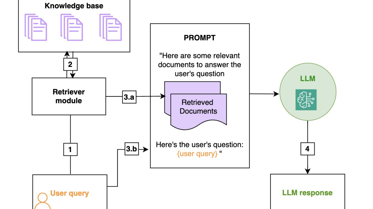


 Sohaib Katariwala is a Sr. Specialist Solutions Architect at AWS focused on Amazon OpenSearch Service. His interests are in all things data and analytics. More specifically he loves to help customers use AI in their data strategy to solve modern day challenges.
 Michael Hamilton is an Analytics & AI Specialist Solutions Architect at AWS. He enjoys all things data related and helping customers solution for their complex use cases.
 Nabil Ezzarhouni is an AI/ML and Generative AI Solutions Architect at AWS. He is based in Austin, TX and passionate about Cloud, AI/ML technologies, and Product Management. When he is not working, he spends time with his family, looking for the best taco in Texas. Because…… why not?

 Shayan Ray is an Applied Scientist at Amazon Web Services. His area of research is all things natural language (like NLP, NLU, NLG). His work has been focused on conversational AI, task-oriented dialogue systems and LLM-based agents. His research publications are on natural language processing, personalization, and reinforcement learning.
 Fangzhou Cheng is a Senior Applied Scientist at AWS. He builds science solutions for AWS Rekgnition and AWS Monitron to provide customers with state-of-the-art models. His areas of focus include generative AI, computer vision, and time-series data analysis
 Marcel Pividal is a Senior AI Services SA in the World- Wide Specialist Organization, bringing over 22 years of expertise in transforming complex business challenges into innovative technological solutions. As a thought leader in generative AI implementation, he specializes in developing secure, compliant AI architectures for enterprise- scale deployments across multiple industries.


 Asheesh Goja is Principal Solutions Architect at AWS. Prior to AWS, Asheesh worked at prominent organizations such as Cisco and UPS, where he spearheaded initiatives to accelerate the adoption of several emerging technologies. His expertise spans ideation, co-design, incubation, and venture product development. Asheesh holds a wide portfolio of hardware and software patents, including a real-time C++ DSL, IoT hardware devices, Computer Vision and Edge AI prototypes. As an active contributor to the emerging fields of Generative AI and Edge AI, Asheesh shares his knowledge and insights through tech blogs and as a speaker at various industry conferences and forums.
 Dhawal Patel is a Principal Machine Learning Architect at AWS. He has worked with organizations ranging from large enterprises to mid-sized startups on problems related to distributed computing, and Artificial Intelligence. He focuses on Deep learning including NLP and Computer Vision domains. He helps customers achieve high performance model inference on SageMaker.
 Greg Benson is a Professor of Computer Science at the University of San Francisco and Chief Scientist at SnapLogic. He joined the USF Department of Computer Science in 1998 and has taught undergraduate and graduate courses including operating systems, computer architecture, programming languages, distributed systems, and introductory programming. Greg has published research in the areas of operating systems, parallel computing, and distributed systems. Since joining SnapLogic in 2010, Greg has helped design and implement several key platform features including cluster processing, big data processing, the cloud architecture, and machine learning. He currently is working on Generative AI for data integration.
 Aaron Kesler is the Senior Product Manager for AI products and services at SnapLogic, Aaron applies over ten years of product management expertise to pioneer AI/ML product development and evangelize services across the organization. He is the author of the upcoming book “What’s Your Problem?” aimed at guiding new product managers through the product management career. His entrepreneurial journey began with his college startup, STAK, which was later acquired by Carvertise with Aaron contributing significantly to their recognition as Tech Startup of the Year 2015 in Delaware. Beyond his professional pursuits, Aaron finds joy in golfing with his father, exploring new cultures and foods on his travels, and practicing the ukulele.
 David Dellsperger is a Senior Staff Software Engineer and Technical Lead of the Agent Creator product at SnapLogic. David has been working as a Software Engineer emphasizing in Machine Learning and AI for over a decade previously focusing on AI in Healthcare and now focusing on the SnapLogic Agent Creator. David spends his time outside of work playing video games and spending quality time with his yellow lab, Sudo


 Jerry Henley, VP of Technology at Curriculum Advantage, leads the product technical vision, platform services, and support for Classworks. With 18 years in EdTech, he oversees innovation, roadmaps, and AI integration, enhancing personalized learning experiences for students and educators.
 Hans Buchheim, VP of Engineering at Curriculum Advantage, has spent 25 years developing Classworks. He leads software architecture decisions, mentors junior developers, and ensures the product evolves to meet educator needs.
 Roy Gunter, DevOps Engineer at Curriculum Advantage, manages cloud infrastructure and automation for Classworks. He focuses on system reliability, troubleshooting, and performance optimization to deliver an excellent user experience.
 Gowtham Shankar is a Solutions Architect at Amazon Web Services (AWS). He is passionate about working with customers to design and implement cloud-native architectures to address business challenges effectively. Gowtham actively engages in various open source projects, collaborating with the community to drive innovation.
 Dr. Changsha Ma is an AI/ML Specialist at AWS. She is a technologist with a PhD in Computer Science, a master’s degree in Education Psychology, and years of experience in data science and independent consulting in AI/ML. She is passionate about researching methodological approaches for machine and human intelligence. Outside of work, she loves hiking, cooking, hunting food, and spending time with friends and families

 Austin Welch is a Senior Applied Scientist at Amazon Web Services Generative AI Innovation Center.
 Bryan Yost is a Principle Deep Learning Architect at Amazon Web Services Generative AI Innovation Center.
 Mehdi Noori is a Senior Applied Scientist at Amazon Web Services Generative AI Innovation Center.


 Daniel Martinez is a Solutions Architect in Iberia Enterprise, part of the worldwide commercial sales organization (WWCS) at AWS.


 Mani Khanuja is a Tech Lead – Generative AI Specialist, author of the book Applied Machine Learning and High Performance Computing on AWS, and a member of the Board of Directors for Women in Manufacturing Education Foundation Board. She leads machine learning projects in various domains such as computer vision, natural language processing, and generative AI. She speaks at internal and external conferences such as AWS re:Invent, Women in Manufacturing West, YouTube webinars, and GHC 23. In her free time, she likes to go for long runs along the beach.
 Erick Friis, Founding Engineer at LangChain, currently spends most of his time on the open source side of the company. He’s an ex-founder with a passion for language-based applications. He spends his free time outdoors on skis or training for triathlons.
 Harrison Chase is the CEO and cofounder of LangChain, an open source framework and toolkit that helps developers build context-aware reasoning applications. Prior to starting LangChain, he led the ML team at Robus Intelligence, led the entity linking team at Kensho, and studied statistics and computer science at Harvard.