Global Resiliency is a new Amazon Lex capability that enables near real-time replication of your Amazon Lex V2 bots in a second AWS Region. When you activate this feature, all resources, versions, and aliases associated after activation will be synchronized across the chosen Regions. With Global Resiliency, the replicated bot resources and aliases in the second Region will have the same identifiers as those in the source Region. This consistency allows you to seamlessly route traffic to any Region by simply changing the Region identifier, providing uninterrupted service availability. In the event of a Regional outage or disruption, you can swiftly redirect your bot traffic to a different Region. Applications now have the ability to use replicated Amazon Lex bots across Regions in an active-active or active-passive manner for improved availability and resiliency. With Global Resiliency, you no longer need to manually manage separate bots across Regions, because the feature automatically replicates and keeps Regional configurations in sync. With just a few clicks or commands, you gain robust Amazon Lex bot replication capabilities. Applications that are using Amazon Lex bots can now fail over from an impaired Region seamlessly, minimizing the risk of costly downtime and maintaining business continuity. This feature streamlines the process of maintaining robust and highly available conversational applications. These include interactive voice response (IVR) systems, chatbots for digital channels, and messaging platforms, providing a seamless and resilient customer experience.
In this post, we walk you through enabling Global Resiliency for a sample Amazon Lex V2 bot. We showcase the replication process of bot versions and aliases across multiple Regions. Additionally, we discuss how to handle integrations with AWS Lambda and Amazon CloudWatch after enabling Global Resiliency.
Solution overview
For this exercise, we create a BookHotel bot as our sample bot. We use an AWS CloudFormation template to build this bot, including defining intents, slots, and other required components such as a version and alias. Throughout our demonstration, we use the us-east-1 Region as the source Region, and we replicate the bot in the us-west-2 Region, which serves as the replica Region. We then replicate this bot, enable logging, and integrate it with a Lambda function.
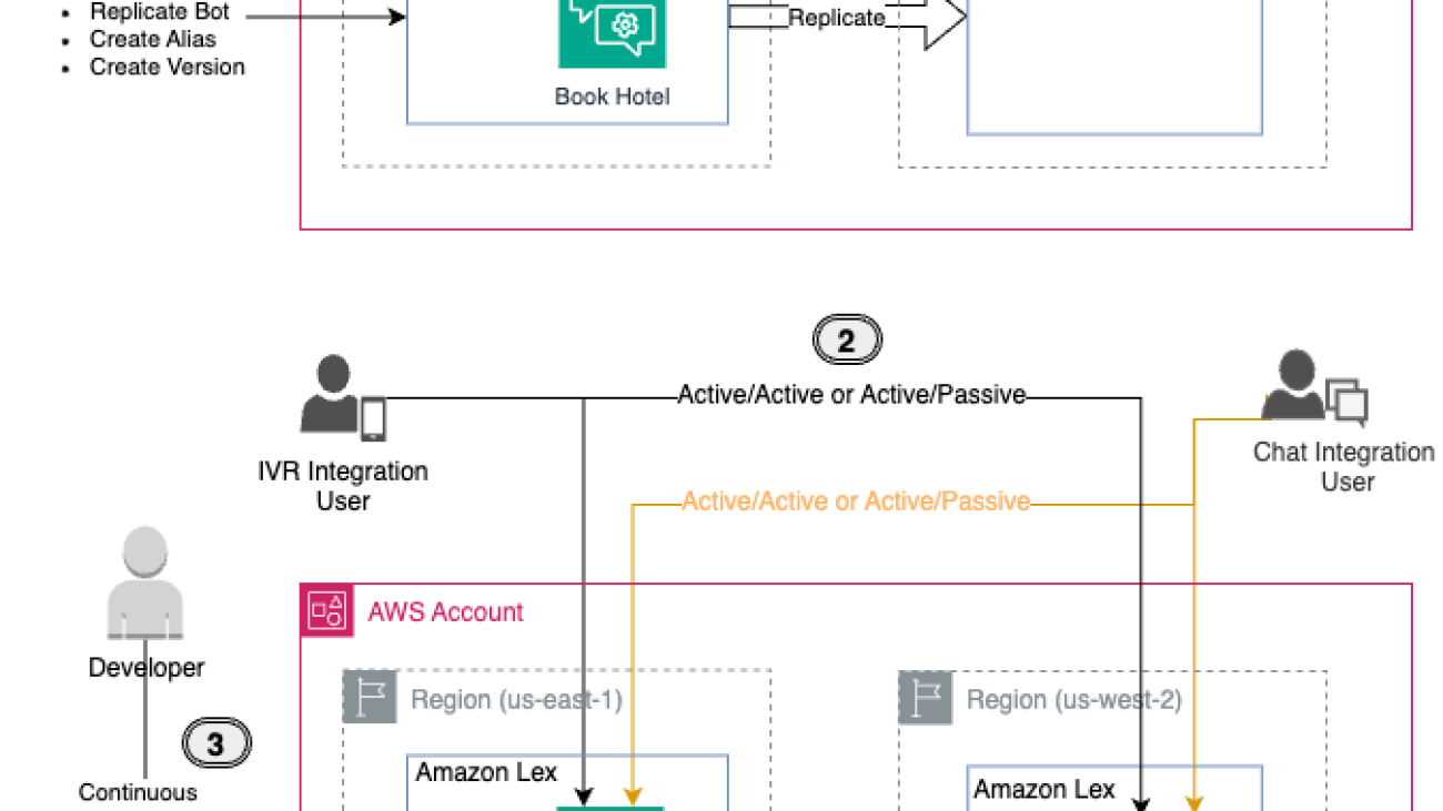
To better understand the solution, refer to the following architecture diagram.

- Enabling Global Resiliency for an Amazon Lex bot is straightforward using the AWS Management Console, AWS Command Line Interface (AWS CLI), or APIs. We walk through the instructions to replicate the bot later in this post.
- After replication is successfully enabled, the bot will be replicated across Regions, providing a unified experience. This allows you to distribute IVR or chat application requests between Regions in either an active-active or active-passive setup, depending on your use case.
- A key benefit of Global Resiliency is that developers can continuously work on bot improvements in the source Region, and changes are automatically synchronized to the replica Region. This streamlines the development workflow without compromising resiliency.
At the time of writing, Global Resiliency only works with predetermined pairs of Regions. For more information, see Use Global Resiliency to deploy bots to other Regions.
Prerequisites
You should have the following prerequisites:
- An AWS account with administrator access
- Access to Amazon Lex Global Resiliency (contact your Amazon Connect Solutions Architect or Technical Account Manager)
- Working knowledge of the following services:
- AWS CloudFormation
- Amazon CloudWatch
- AWS Lambda
- Amazon Lex
Create a sample Amazon Lex bot
To set up a sample bot for our use case, refer to Manage your Amazon Lex bot via AWS CloudFormation templates. For this example, we create a bot named BookHotel in the source Region (us-east-1). Complete the following steps:
- Download the CloudFormation template and deploy it in the source Region (
us-east-1). For instructions, see Create a stack from the CloudFormation console.
Upon successful deployment, the BookHotel bot will be created in the source Region.
- On the Amazon Lex console, choose Bots in the navigation pane and locate the BookHotel.
Verify that the Global Resiliency option is available under Deployment in the navigation pane. If this option isn’t visible, the Global Resiliency feature may not be enabled for your account. In this case, refer to the prerequisites section for enabling the Global Resiliency feature.

Our sample BookHotel bot has one version (Version 1, in addition to the draft version) and an alias named BookHotelDemoAlias (in addition to the TestBotAlias).
Enable Global Resiliency
To activate Global Resiliency and set up bot replication in a replica Region, complete the following steps:
- On the Amazon Lex console, choose
us-east-1as your Region. - Choose Bots in the navigation pane and locate the BookHotel.
- Under Deployment in the navigation pane, choose Global Resiliency.
You can see the replication details here. Because you haven’t enabled Global Resiliency yet, all the details are blank.
- Choose Create replica to create a draft version of your bot.

In your source Region (us-east-1), after the bot replication is complete, you will see Replication status as Enabled.
- Switch to the replica Region (
us-west-2).
You can see that the BookHotel bot is replicated. This is a read-only replica and the bot ID in the replica Region matches the bot ID in the source Region.
- Under Deployment in the navigation pane, choose Global Resiliency.
You can see the replication details here, which are the same as that in the source Region BookHotel bot.
You have verified that the bot is replicated successfully after Global Resiliency is enabled. Only new versions and aliases created from this point onward will be replicated. As a next step, we create a bot version and alias to demonstrate the replication.
Create a new bot version and alias
Complete the following steps to create a new bot version and alias:
- On the Amazon Lex console in your source Region (
us-east-1), navigate to the BookHotel. - Choose Bot versions in the navigation pane, and choose Create new version to create Version 2.
Version 2 now has Global Resiliency enabled, whereas Version 1 and the draft version do not, because they were created prior to enabling Global Resiliency.
- Choose Aliases in the navigation pane, then choose Create new alias.
- Create a new alias for the BookHotel bot called
BookHotelDemoAlias_GRand point that to the new version.
Similarly, the BookHotelDemoAlias_GR now has Global Resiliency enabled, whereas aliases created before enabling Global Resiliency, such as BookHotelDemoAlias and TestBotAlias, don’t have Global Resiliency enabled.
- Choose Global Resiliency in the navigation pane to view the source and replication details.
The details for Last replicated version are now updated to Version 2.
- Switch to the replica Region (
us-west-2) and choose Global Resiliency in the navigation pane.
You can see that the new Global Resiliency enabled version (Version 2) is replicated and the new alias BookHotelDemoAlias_GR is also present.
You have verified that the new version and alias were created after Global Resiliency is replicated to the replica Region. You can now make Amazon Lex runtime calls to both Regions.
Handling integrations with Lambda and CloudWatch after enabling Global Resiliency
Amazon Lex has integrations with other AWS services such as enabling custom logic with Lambda functions and logging with conversation logs using CloudWatch and Amazon Simple Storage Service (Amazon S3). In this section, we associate a Lambda function and CloudWatch group for the BookHotel bot in the source Region (us-east-1) and validate its association in the replica Region (us-west-2).
- Download the CloudFormation template to deploy a sample Lambda and CloudWatch log group.
- Deploy the CloudFormation stack to the source Region (
us-east-1). For instructions, see Create a stack from the CloudFormation console.
This will deploy a Lambda function (book-hotel-lambda) and a CloudWatch log group (/lex/book-hotel-bot) in the us-east-1 Region.
- Deploy the CloudFormation stack to the replica Region (
us-west-2).
This will deploy a Lambda function (book-hotel-lambda) and a CloudWatch log group (/lex/book-hotel-bot) in the us-west-2 Region. The Lambda function name and CloudWatch log group name must be the same in both Regions.
- On the Amazon Lex console in the source Region (
us-east-1), navigate to the BookHotel. - Choose Aliases in the navigation pane, and choose the
BookHotelDemoAlias_GR. - In the Languages section, choose English (US).
- Select the
book-hotel-lambdafunction and associate it with the BookHotel bot by choosing Save. - Navigate back to the
BookHotelDemoAlias_GRalias, and in the Conversation logs section, choose Manage conversation logs. - Enable Text logs and select the
/lex/book-hotel-bot loggroup, then choose Save.
Conversation text logs are now enabled for the BookHotel bot in us-east-1.
- Switch to the replica Region (
us-west-2) and navigate to the BookHotel. - Choose Aliases in the navigation pane, and choose the
BookHotelDemoAlias_GR.
You can see that the conversation logs are already associated with the /lex/book-hotel-bot CloudWatch group the us-west-2 Region.
- In the Languages section, choose English (US).
You can see that the book-hotel-lambda function is associated with the BookHotel alias.
Through this process, we have demonstrated how Lambda functions and CloudWatch log groups are automatically associated with the corresponding bot resources in the replica Region for the replicated bots, providing a seamless and consistent integration across both Regions.
Disabling Global Resiliency
You have the flexibility to disable Global Resiliency at any time. By disabling Global Resiliency, your source bot, along with its associated aliases and versions, will no longer be replicated across other Regions. In this section, we demonstrate the process to disable Global Resiliency.
- On the Amazon Lex console in your source Region (
us-east-1), choose Bots in the navigation pane and locate the BookHotel. - Under Deployment in the navigation pane, choose Global Resiliency.
- Choose Disable Global Resiliency.

- Enter confirm in the confirmation box and choose Delete.
This action initiates the deletion of the replicated BookHotel bot in the replica Region.
The replication status will change to Deleting, and after a few minutes, the deletion process will be complete. You will then see the Create replica option available again. If you don’t see it, try refreshing the page.

- Check the Bot versions page of the BookHotel bot to confirm that Version 2 is still the latest version.
- Check the Aliases page to confirm that the
BookHotelDemoAlias_GRalias is still present on the source bot.
Applications referring to this alias can continue to function as normal in the source Region.
- Switch to the replica Region (
us-west-2) to confirm that the BookHotel bot has been deleted from this Region.
You can reenable Global Resiliency on the source Region (us-east-1) by going through the process described earlier in this post.
Clean up
To prevent incurring charges, complete the following steps to clean up the resources created during this demonstration:
- Disable Global Resiliency for the bot by following the instructions detailed earlier in this post.
- Delete the
book-hotel-lambda-cw-stackCloudFormation stack from theus-west-2. For instructions, see Delete a stack on the CloudFormation console. - Delete the
book-hotel-lambda-cw-stackCloudFormation stack from theus-east-1. - Delete the
book-hotel-stackCloudFormation stack from theus-east-1.
Integrations with Amazon Connect
Amazon Lex Global Resiliency seamlessly complements Amazon Connect Global Resiliency, providing you with a comprehensive solution for maintaining business continuity and resilience across your conversational AI and contact center infrastructure. Amazon Connect Global Resiliency enables you to automatically maintain your instances synchronized across two Regions, making sure that all configuration resources, such as contact flows, queues, and agents, are true replicas of each other.
With the addition of Amazon Lex Global Resiliency, Amazon Connect customers gain the added benefit of automated synchronization of their Amazon Lex V2 bots associated with their contact flows. This integration provides a consistent and uninterrupted experience during failover scenarios, because your Amazon Lex interactions seamlessly transition between Regions without any disruption. By combining these complementary features, you can achieve end-to-end resilience. This minimizes the risk of downtime and makes sure your conversational AI and contact center operations remain highly available and responsive, even in the case of Regional failures or capacity constraints.
Global Resiliency APIs
Global Resiliency provides API support to create and manage replicas. These are supported in the AWS CLI and AWS SDKs. In this section, we demonstrate usage with the AWS CLI.
- Create a bot replica in the replica Region using the CreateBotReplica.
- Monitor the bot replication status using the DescribeBotReplica.
- List the replicated bots using the ListBotReplicas.
- List all the version replication statuses applicable for Global Resiliency using the ListBotVersionReplicas.
This list includes only the replicated bot versions, which were created after Global Resiliency was enabled. In the API response, a botVersionReplicationStatus of Available indicates that the bot version was replicated successfully.
- List all the alias replication statuses applicable for Global Resiliency using the ListBotAliasReplicas.
This list includes only the replicated bot aliases, which were created after Global Resiliency was enabled. In the API response, a botAliasReplicationStatus of Available indicates that the bot alias was replicated successfully.
Conclusion
In this post, we introduced the Global Resiliency feature for Amazon Lex V2 bots. We discussed the process to enable Global Resiliency using the console and reviewed some of the new APIs released as part of this feature.
As the next step, you can explore Global Resiliency and apply the techniques discussed in this post to replicate bots and bot versions across Regions. This hands-on practice will solidify your understanding of managing and replicating Amazon Lex V2 bots in your solution architecture.
About the Authors
 Priti Aryamane is a Specialty Consultant at AWS Professional Services. With over 15 years of experience in contact centers and telecommunications, Priti specializes in helping customers achieve their desired business outcomes with customer experience on AWS using Amazon Lex, Amazon Connect, and generative AI features.
 Sanjeet Sanda is a Specialty Consultant at AWS Professional Services with over 20 years of experience in telecommunications, contact center technology, and customer experience. He specializes in designing and delivering customer-centric solutions with a focus on integrating and adapting existing enterprise call centers into Amazon Connect and Amazon Lex environments. Sanjeet is passionate about streamlining adoption processes by using automation wherever possible. Outside of work, Sanjeet enjoys hanging out with his family, having barbecues, and going to the beach.
 Yogesh Khemka is a Senior Software Development Engineer at AWS, where he works on large language models and natural language processing. He focuses on building systems and tooling for scalable distributed deep learning training and real-time inference.


 Kara Yang is a Data Scientist at AWS Professional Services in the San Francisco Bay Area, with extensive experience in AI/ML. She specializes in leveraging cloud computing, machine learning, and Generative AI to help customers address complex business challenges across various industries. Kara is passionate about innovation and continuous learning.
 Farshad Harirchi is a Principal Data Scientist at AWS Professional Services. He helps customers across industries, from retail to industrial and financial services, with the design and development of generative AI and machine learning solutions. Farshad brings extensive experience in the entire machine learning and MLOps stack. Outside of work, he enjoys traveling, playing outdoor sports, and exploring board games.
 James Poquiz is a Data Scientist with AWS Professional Services based in Orange County, California. He has a BS in Computer Science from the University of California, Irvine and has several years of experience working in the data domain having played many different roles. Today he works on implementing and deploying scalable ML solutions to achieve business outcomes for AWS clients.

 Ishan Singh is a Generative AI Data Scientist at Amazon Web Services, where he helps customers build innovative and responsible generative AI solutions and products. With a strong background in AI/ML, Ishan specializes in building Generative AI solutions that drive business value. Outside of work, he enjoys playing volleyball, exploring local bike trails, and spending time with his wife and dog, Beau.
 Chris Pecora is a Generative AI Data Scientist at Amazon Web Services. He is passionate about building innovative products and solutions while also focused on customer-obsessed science. When not running experiments and keeping up with the latest developments in generative AI, he loves spending time with his kids.
 Yanyan Zhang is a Senior Generative AI Data Scientist at Amazon Web Services, where she has been working on cutting-edge AI/ML technologies as a Generative AI Specialist, helping customers use generative AI to achieve their desired outcomes. Yanyan graduated from Texas A&M University with a PhD in Electrical Engineering. Outside of work, she loves traveling, working out, and exploring new things.
 Mani Khanuja is a Tech Lead – Generative AI Specialists, author of the book Applied Machine Learning and High Performance Computing on AWS, and a member of the Board of Directors for Women in Manufacturing Education Foundation Board. She leads machine learning projects in various domains such as computer vision, natural language processing, and generative AI. She speaks at internal and external conferences such AWS re:Invent, Women in Manufacturing West, YouTube webinars, and GHC 23. In her free time, she likes to go for long runs along the beach.


 Neeraj Lamba is a Cloud Infrastructure Architect with Amazon Web Services (AWS) Worldwide Public Sector Professional Services. He helps customers transform their business by helping design their cloud solutions and offering technical guidance. Outside of work, he likes to travel, play Tennis and experimenting with new technologies.
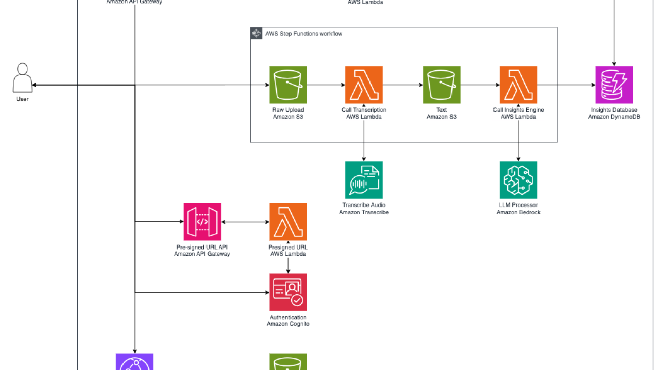


 Simone Zucchet is a Solutions Architect Manager at AWS. With over 6 years of experience as a Cloud Architect, Simone enjoys working on innovative projects that help transform the way organizations approach business problems. He helps support large enterprise customers at AWS and is part of the Machine Learning TFC. Outside of his professional life, he enjoys working on cars and photography.
 Vu San Ha Huynh is a Solutions Architect at AWS. He has a PhD in computer science and enjoys working on different innovative projects to help support large enterprise customers.
 Adam Raffe is a Principal Solutions Architect at AWS. With over 8 years of experience in cloud architecture, Adam helps large enterprise customers solve their business problems using AWS.
 Ahmed Raafat is a Principal Solutions Architect at AWS, with 20 years of field experience and a dedicated focus of 6 years within the AWS ecosystem. He specializes in AI/ML solutions. His extensive experience spans various industry verticals, making him a trusted advisor for numerous enterprise customers, helping them seamlessly navigate and accelerate their cloud journey.


 Erik Cordsen is a Solutions Architect at AWS serving customers in Georgia. He is passionate about applying cloud technologies and ML to solve real life problems. When he is not designing cloud solutions, Erik enjoys travel, cooking, and cycling.
 Vivek Mittal is a Solution Architect at Amazon Web Services. He is passionate about serverless and machine learning technologies. Vivek takes great joy in assisting customers with building innovative solutions on the AWS cloud.
 Brijesh Pati is an Enterprise Solutions Architect at AWS. His primary focus is helping enterprise customers adopt cloud technologies for their workloads. He has a background in application development and enterprise architecture and has worked with customers from various industries such as sports, finance, energy, and professional services. His interests include serverless architectures and AI/ML.


 Amit Gautam is an AWS senior solutions architect supporting enterprise customers in the UK on their cloud journeys, providing them with architectural advice and guidance that helps them achieve their business outcomes.
 Sujata Singh is an AWS senior solutions architect supporting enterprise customers in the UK on their cloud journeys, providing them with architectural advice and guidance that helps them achieve their business outcomes.


 Joe King is a Sr. Data Scientist at AWS, bringing a breadth of data science, ML engineering, MLOps, and AI/ML architecting to help businesses create scalable solutions on AWS.
 Ajay Raghunathan is a Machine Learning Engineer at AWS. His current work focuses on architecting and implementing ML solutions at scale. He is a technology enthusiast and a builder with a core area of interest in AI/ML, data analytics, serverless, and DevOps. Outside of work, he enjoys spending time with family, traveling, and playing football.
 Raju Patil is a Sr. Data Scientist with AWS Professional Services. He architects, builds, and deploys AI/ML solutions to help AWS customers across different verticals overcome business challenges in a variety of AI/ML use cases.


 Sunil Ramachandra is a Senior Solutions Architect enabling hyper-growth Independent Software Vendors (ISVs) to innovate and accelerate on AWS. He partners with customers to build highly scalable and resilient cloud architectures. When not collaborating with customers, Sunil enjoys spending time with family, running, meditating, and watching movies on Prime Video.
 Benedict Augustine is a thought leader in Generative AI and Machine Learning, serving as a Senior Specialist at AWS. He advises customer CxOs on AI strategy, to build long-term visions while delivering immediate ROI.As VP of Machine Learning, Benedict spent the last decade building seven AI-first SaaS products, now used by Fortune 100 companies, driving significant business impact. His work has earned him 5 patents.
 Lee Rehwinkel is a Principal Data Scientist at Planview with 20 years of experience in incorporating AI & ML into Enterprise software. He holds advanced degrees from both Carnegie Mellon University and Columbia University. Lee spearheads Planview’s R&D efforts on AI capabilities within Planview Copilot. Outside of work, he enjoys rowing on Austin’s Lady Bird Lake.