Generative AI continues to push the boundaries of what’s possible. One area garnering significant attention is the use of generative AI to analyze audio and video transcripts, increasing our ability to extract valuable insights from content stored in audio or video files. Speech data is unique and complex, which makes it difficult to analyze and extract insights. Manually transcribing and analyzing it can be time-consuming and resource-intensive.
Existing methods for extracting insights from speech data often require tedious human transcription and review. You can use automatic voice recognition tools to convert your audio and video data to text. However, you still have to rely on manual processes for extracting specific insights and data points, or get summaries of the content. This approach is time-consuming and as organizations amass vast amounts of this content, the need for a more efficient and insightful solution becomes increasingly pressing. There is a significant opportunity to add business value given the amount of data organizations store in these formats and the valuable insights that might otherwise go undiscovered. The following are some of the new insights and capabilities that can be obtained through the use of large language models (LLM) with audio transcripts:
- LLMs can analyze and understand the context of a conversation, not just the words spoken, but also the implied meaning, intent, and emotions. Previously, this would have required extensive human interpretation.
- LLMs can perform advanced sentiment analysis. Previously, sentiment analysis could be captured, but LLMs can capture more emotions, such as sarcasm, ambivalence, or mixed feelings by understanding the context of the conversation.
- LLMs can generate concise summarizations not just by extracting content, but by understanding the context of the conversation.
- Users can now ask complex, natural language questions and receive insightful answers.
- LLMs can infer personas or roles in a conversation, enabling targeted insights and actions.
- LLMs can support the creation of new content based on audio assets or conversations following predetermined templates or flows.
In this post, we examine how to create business value through speech analytics with some examples focused on the following:
- Automatically summarizing, categorizing, and analyzing marketing content such as podcasts, recorded interviews, or videos, and creating new marketing materials based on those assets
- Automatically extracting key points, summaries, and sentiment from a recorded meeting (such as an earnings call)
- Transcribing and analyzing contact center calls to improve customer experience.
The first step in getting these audio data insights involves transcribing the audio file using Amazon Transcribe. Amazon Transcribe is a machine learning (ML) based managed service that automatically converts speech to text, enabling developers to seamlessly integrate speech-to-text capabilities into their applications. It also recognizes multiple speakers, automatically redacts personally identifiable information (PII), and allows you to enhance the accuracy of a transcription by providing custom vocabularies specific to your industries or use case, or by using custom language models.
The second step involves using foundation models (FMs) with Amazon Bedrock to summarize the content, identify topics, and recognize conclusions, extracting valuable insights that can guide strategic decisions and innovations. Automatic generation of new content also adds value, increasing creativity and productivity.
Generative AI is reshaping the way we analyze audio transcripts, enabling you to unlock insights such as customer sentiment, pain points, common themes, avenues for risk mitigation, and more, that were previously obfuscated.
Use case overview
In this post, we discuss three example use cases in detail. The code artifacts are in Python. We used a Jupyter notebook to run the code snippets. You can follow along by creating and running a notebook in Amazon SageMaker Studio.
Audio summarization and insights, and automated generation of new content using Amazon Transcribe and Amazon Bedrock
Through this use case, we demonstrate how to take an existing marketing asset (a video) and create a new blog post to announce the launch of the video, create an abstract, and extract the main topics and the search engine optimization (SEO) keywords present in the post for documenting and categorizing the asset.
Transcribe audio with Amazon Transcribe
In this case, we use an AWS re:Invent 2023 technical talk as a sample. For the purpose of this notebook, we downloaded the MP4 file for the recording and stored it in an Amazon Simple Storage Service (Amazon S3) bucket.
The first step is to transcribe the audio file using Amazon Transcribe:
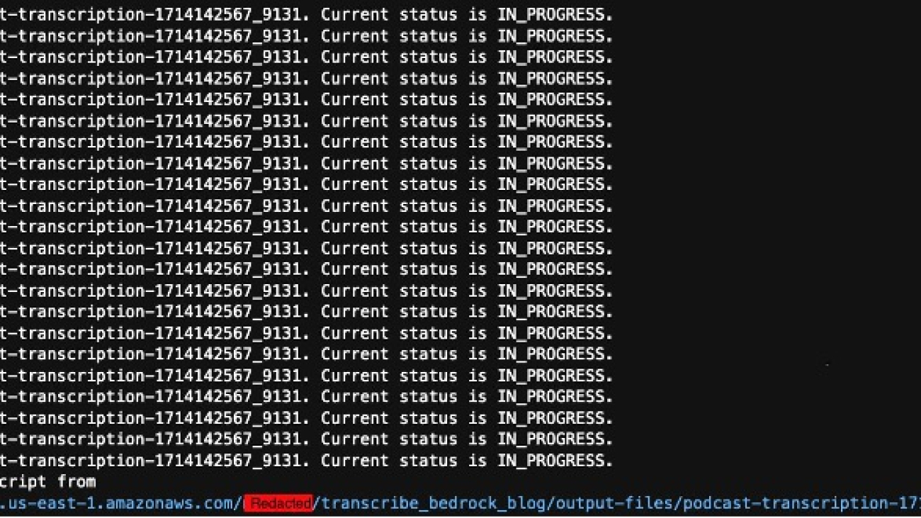
The transcription job will take a few minutes to complete.
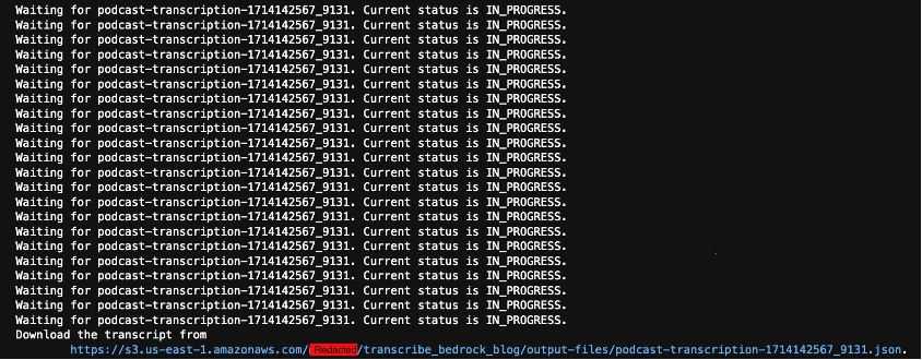
When the job is complete, you can inspect the transcription output and check the plain text transcript that was generated (the following has been trimmed for brevity):
……….Once the alert comes, how do you kind of correlate these alerts, not by just text signals and text passing, but understanding the topology, the infrastructure topology that is supporting that application or that business service. It is the topology that ultimately gives the source of truth when an alert comes, right. That’s what we mean by a correlation that is assisted with topology in in in the thing that ultimately results in finding a probable root cause. And once ……….
After you have validated the existence of the text, you can use Amazon Bedrock to analyze the output:
Using the transcription from the technical talk, we use Amazon Bedrock to call an FM (we use Anthropic’s Claude 3 Sonnet on Amazon Bedrock in this case). You can choose from the language models available on Amazon Bedrock from AI21 Labs, Anthropic, Cohere, Meta, Mistral AI, Stability AI, and Amazon.
You can now perform additional tasks.
Extract the main topics with Amazon Bedrock
The following prompt provides instructions to ask the LLM for the main topics in the technical talk:
We have created a prompt that uses prompting best practices for Anthropic’s Claude. In this case, we pass the transcript within the <transcript></transcript> XML tags and ask for main topics discussed. Based on that, we get the following output:
Based on the contents of the transcript, the main topics being discussed are:
- AI and Machine Learning in IT Operations
- Challenges faced by IT Operations teams
- Observable data explosion from cloud, on-premise, and edge infrastructure
- The convergence of IT, SRE, and DevOps roles
- Discovery to Resolution pipeline for IT Operations
- Alert correlation and intelligent alerting using AI/ML
- Probable root cause analysis with AI/ML
- Automated remediation and runbook automation
- Predictive analytics and preventive maintenance using AI/ML
- Benefits of AI/ML for IT Operations (proactive operations, reduced human effort, improved service health, cost optimization)
Generate a blog post to announce the video with Amazon Bedrock
The following prompt provides instructions to ask the LLM for the generation of a new blog post announcing the launch of the preceding recording. Just like the preceding prompt, we use prompting best practices for Anthropic’s Claude:
Based on that, we get the following output:
Here is a draft 1462 word blogpost summarizing the technical talk and announcing the recording is now available:
Title: Revolutionizing IT Operations with AI/ML: A Future-Ready Approach
The world of IT operations is undergoing a seismic shift, driven by the explosion of observable data, the convergence of IT roles, and the advent of hybrid multi-cloud environments. Traditional reactive approaches are no longer sufficient to keep pace with the complexity and scale of modern IT systems. This is where AI and machine learning (ML) come into play, offering a future-ready approach to revolutionize IT operations.
In a recent technical talk, Verma from HPE OpsRamp outlined the drivers behind this AI/ML imperative and demonstrated how this cutting-edge technology is fundamentally transforming IT operations. The recording of this insightful session is now available for public consumption.
The Drivers Behind the AI/ML Imperative
The first driving force behind the adoption of AI/ML in IT operations is the sheer volume of observable data that………………..
Create an abstract with Amazon Bedrock
The following prompt provides instructions to create an abstract summarizing the content of the technical talk:
Based on this, we get the following output:
Here is a 96 word abstract for the technical talk:
This talk discussed how AI and machine learning innovations are transforming IT operations for hybrid multi-cloud workloads. The speakers outlined the challenges of dealing with exploding observable data from modern infrastructure and the convergence of IT roles. They demonstrated how AI/ML techniques like intelligent alerting, alert correlation, probable root cause analysis, and automated remediation can drive more proactive, predictive operations. Key benefits showcased included reduced human effort, improved service health, and cost optimization. The talk featured a demo of the OpsRamp platform leveraging AI/ML models to streamline the discovery-to-resolution pipeline for managing edge-to-cloud environments.
Extract SEO keywords from the generated blog post with Amazon Bedrock
The following prompt provides instructions to extract the main SEO keywords from the generated blog post. Based on online research on how to extract SEO keywords from long-form text, we came up with the following list. This demonstrates how you can empower an LLM like Anthropic’s Claude to follow instructions and best practices for a particular task or domain. Also, the prompt specifies that the output should be in JSON. This is helpful in use cases where you want to programmatically get results from an LLM and therefore require consistent formatting. Based on best practices for Anthropic’s Claude, we use the Assistant message in the messages API to pre-fill the model’s response to have further control on the output format:
Based on this, we get the following output:
{‘keywords’: [‘AI-driven IT operations’, ‘machine learning IT operations’, ‘proactive IT operations’, ‘predictive IT operations’, ‘AI for hybrid cloud’, ‘AI for multi-cloud’, ‘FutureOps’, ‘AI-assisted IT operations’, ‘AI-powered event correlation’, ‘intelligent alerting’, ‘automated remediation workflows’, ‘predictive analytics for IT’, ‘AI anomaly detection’, ‘AI root cause analysis’, ‘AI-driven observability’, ‘AI for DevOps’, ‘AI for SRE’, ‘AI IT operations management’]}
For consistent formatting and structured output, you can also use the Converse and ConverseStream APIs in Amazon Bedrock and use the tool calling capabilities of the LLMs that offer it.
Generate a new blog post version emphasizing specific SEO keywords with Amazon Bedrock
The following prompt provides instructions to generate a new blog post emphasizing three keywords or phrases from the ones extracted in the previous step. In this case, we use the first three keywords in the returned keywords list. The instructions specified in the prompt are derived from SEO content best practices:
Based on this, we get the following output:
<blog>
Title: Unleash the Power of AI-Driven and Machine Learning IT Operations for Proactive IT Operations
In today’s rapidly evolving digital landscape, traditional IT operations approaches are struggling to keep pace. The explosion of data from cloud workloads, Kubernetes clusters, and distributed edge locations has overwhelmed conventional monitoring tools, leading to fragmented views and reactive operations that respond to issues after they occur. To stay ahead of the curve, organizations must embrace AI-driven and machine learning IT operations, paving the way for proactive IT operations that enhance efficiency and minimize downtime.
At a recent technical talk, Verma and Radha Krishna Kunni from OpsRamp (recently acquired by HPE) delved into the transformative impact of AI and machine learning on IT operations, DevOps, and SRE for hybrid multi-cloud environments. They highlighted the key challenges ops teams face today and introduced the innovative “FutureOps” approach, which leverages AI and machine learning to revolutionize IT operations.
The full video recording of this insightful technical talk is now available [link], providing a comprehensive understanding of…………
Summarize content discussed in a recorded meeting using Amazon Transcribe and Amazon Bedrock
Through this use case, we demonstrate how to take an existing recording from a meeting (we use a recording from an AWS earnings call) to summarize the content discussed, extract the key points, and provide details on the sentiment of the meeting. For additional information on this use case, see Live Meeting Assistant with Amazon Transcribe, Amazon Bedrock, and Amazon Bedrock Knowledge Bases or Amazon Q Business.
Transcribe audio with Amazon Transcribe
In this use case, we use an Amazon 2024 Q1 earnings call as a sample. For the purpose of this notebook, we downloaded the WAV file for the recording and stored in an S3 bucket.
The first step is to transcribe the audio file using Amazon Transcribe:
The transcription job will take a few minutes to complete.
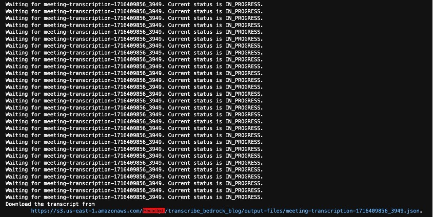
When the job is complete, you can inspect the transcription output and check for the plain text transcript that was generated:
Thank you for standing by. Good day, everyone and welcome to the amazon.com first quarter, 2024 financial results teleconference. At this time, all participants are in a listen only mode. After the presentation, we will conduct a question and answer session. Today’s call is being recorded and for opening remarks, I’ll be turning the call over to the Vice President of Investor………
After you have validated the existence of the text, you can use Amazon Bedrock to analyze the output:
Using the transcription from the earnings call recording, we use Amazon Bedrock to call an FM (we use Anthropic’s Claude 3 Sonnet in this case). You can choose from other FMs available on Amazon Bedrock.
You can now perform additional tasks.
Identify the financial ratios highlighted during this earnings call
The following prompt provides instructions to identify financial ratios highlighted during the earnings call and their implications:
Based on this, we get the following output:
Based on the earnings call transcript, the following financial ratios and their implications were highlighted:
- Operating Income Margin:
- Amazon reported its highest ever quarterly operating income of $15.3 billion, which was $3.3 billion above the high end of their guidance range. This was driven by strong operational performance across all three reportable segments (North America, International, and AWS) and better-than-expected operating leverage, including lower cost to serve.
- North America segment operating income was $5 billion with an operating margin of 5.8%, up 460 basis points year-over-year, driven by improvements in cost to serve, including benefits from regionalization efforts, more consolidated customer shipments, and improved leverage.
- International segment operating income was $903 million with an operating margin of 2.8%, up 710 basis points year-over-year, primarily driven by cost efficiencies through network design enhancements and improved volume leverage in established countries, as well as progress in emerging countries.
- AWS operating income was $9.4 billion, an increase of $4.3 billion year-over-year, with improved leverage from managing infrastructure and fixed costs while growing at a healthy rate.
Implication: The higher operating income margins across all segments indicate Amazon’s focus on driving efficiencies and improving profitability while continuing to invest in growth opportunities.
- Revenue Growth:
- Worldwide revenue was $143.3 billion, up 13% year-over-year (excluding the impact of foreign exchange).
- AWS revenue grew 17.2% year-over-year, accelerating from 13.2% in Q4 2023, driven by strong demand for both generative AI and non-generative AI workloads.
- Advertising revenue grew 24% year-over-year (excluding the impact of foreign exchange), primarily driven by sponsored products and improvements in relevancy and measurement capabilities.
Implication: The strong revenue growth, particularly in AWS and advertising, highlights Amazon’s diversified revenue streams and the growth opportunities in cloud computing and digital advertising.
- Capital Expenditures (Capex):
- Amazon anticipates a meaningful increase in overall capital expenditures in 2024, primarily driven by higher infrastructure Capex for growth in AWS, including generative AI investments.
- In Q1 2024, Capex was $14 billion, expected to be the lowest quarter of the year.
Implication: The increase in Capex signals Amazon’s confidence in the strong demand for AWS and their commitment to investing in emerging technologies like generative AI to drive future growth.
Overall, the financial ratios and commentary indicate Amazon’s focus on improving profitability, driving operational efficiencies, and investing in growth opportunities, particularly in AWS and generative AI, while maintaining a diversified revenue stream and managing costs effectively.
Identify the speakers from the earnings call with Amazon Bedrock
The following prompt provides instructions to identify the speakers in the meeting from the transcription:
Based on this, we get the following output:
Based on the transcript, the key speakers on this Amazon earnings call appear to be:
- Andy Jassy – CEO of Amazon
- Brian Olsavsky – CFO of Amazon
- Dave Fildes – Vice President of Investor Relations at Amazon
The call begins with opening remarks from Dave Fildes, followed by prepared statements from Andy Jassy and Brian Olsavsky. They then take questions from analysts, with Andy and Brian providing the responses.
Obtain the challenges or negative areas discussed on the earnings call with Amazon Bedrock
The following prompt provides instructions to obtain the challenges or negative areas discussed from the transcription:
Based on this, we get the following output:
Based on the transcript, some of the key challenges or negative areas discussed include:
- Foreign exchange headwinds: Amazon faced an unfavorable impact from global currencies weakening against the U.S. dollar in Q1, leading to a $700 million or 50 basis point headwind to revenue compared to guidance.
- Increasing capital expenditures: Amazon expects to meaningfully increase its capital expenditures year-over-year in 2024, primarily driven by higher infrastructure spending for AWS growth, including investments in generative AI capabilities.
- Consumer spending concerns: Amazon mentioned keeping an eye on consumer spending trends, specifically in Europe, where it appears weaker relative to the U.S.
- International segment profitability: While the international segment’s profitability improved, with an operating margin of 2.8%, Amazon acknowledged the need to continue working on cost efficiencies and profitability, particularly in emerging countries.
- Cost optimization challenges: Although Amazon believes the majority of cost optimization efforts are behind them, there is still a need to continually streamline processes, optimize inventory placement, and invest in automation to further reduce the cost to serve.
Overall, the challenges centered around foreign exchange impacts, increasing capital intensity for AWS and generative AI investments, consumer demand uncertainties, and ongoing efforts to improve operational efficiencies and international profitability.
Get insights from a call center call between an agent and a customer using Amazon Transcribe and Amazon Bedrock
Through this use case, we demonstrate how to take an existing call recording from a contact center and summarize the content discussed, extract the main topic, key phrases, call reason, customer satisfaction, overall call sentiment, and sentiment about the products and services discussed. For additional details about this use case, see Live call analytics and agent assist for your contact center with Amazon language AI services and Post call analytics for your contact center with Amazon language AI services.
Transcribe audio with Amazon Transcribe
The first step is to transcribe the audio file using Amazon Transcribe. In this case, we use a sample from the Amazon Transcribe Post Call Analytics Solution GitHub repository. For the purpose of this notebook, we downloaded the WAV file and stored it in an S3 bucket.
The transcription job will take a few minutes to complete.
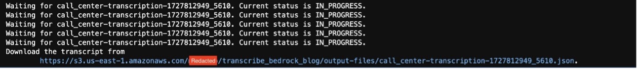
When the job’s complete, you can inspect the transcription output and check for the plain text transcript that was generated:
Thank you for calling Big Jim’s Auto. This is Travis. How can I help you today? Hello, my name is Violet King and I bought a car not too long ago and a light is coming on um a light on the dashboard. And so I was wondering what I should do about that. Ok. It may depend on what kind of light we’re looking at here today, ma’am. Uh Could I get your first and last name spelled out for me so I can just get some information pulled up? Yes. My name is Violet Vviolet. My last name is King King. Ok, I got the call last week. Ok. Uh And what kind of car are we examining today? It’s, it’s a Ford Fusion. It’s 2017, 2017 Ford Fusion. OK. And for verification, ma’am. Do you happen to know the purchase date of the car? Yes, it, it, it was last Tuesday, August 10th. You say the 10th? Ok. And can you describe to me what kind of light we’re looking at? Y yes, it’s uh I, I think it’s a, an oil, an oil light, an oil light? Ok. Ok. And uh just for clarity on my end, ma’am. Um, uh, is this the first call you’ve made regarding this? Yes. Ok. And, uh, this might be kind of a silly question because I know you just got the car. But sometimes they make me ask a silly question about how many miles has the car been driven since you bought it? Oh. I’m not sure. Should I check? Uh, no, that’s ok. I’ll just, I’ll just put in that. We don’t know at this time. It’s ok. Um, so, um, uh, under the warranty we offer, um, we, the, we don’t handle in house oil changes. Um, we basically, when, when someone buys a car from us, the warranty, we have, it, it covers some stuff like, um, weather damage. Um, and, uh, if the engine light comes on, we take a look at that, but the oil change is something that we just don’t have, uh, here at the dealership that’s a little bit outsourced out and they’re pretty backed up right now because a lot of people have been, uh, staying in due to the recent pandemic and now everyone’s just starting to get out and a whole bunch of places are just completely bogged down. So we have a place that we typically outsource to, um, and they’re, they’re pretty reasonable. They’re about, I wanna say somewhere between 25 and $35 to do an oil change. So it’s really not that bad, but they’re a little bit backed up right now from what I’ve heard, I would recommend giving them a call as soon as you can before they close. Ok. What is their number? Uh, give me a second. Let me just rustle through the desk here. See if I can find their information. Uh, ok. Ok. Yes, I’m all right with them one moment, please. Sure. Ok. All their number is 888 333 2222. Ok, and they can fix my car. Yeah, they should be able to handle the oil change. I’m sorry, that’s not something that we cover under the warranty that uh, we have, um, but they should be able to get you settled and, uh, sorted. Ok. Ok. Thank you. Cool. No problem. Have a good one. Thank you. Yup. Bye.
After you have validated the existence of the text, you can use Amazon Bedrock to analyze the output:
Using the transcription from the recorded call center call, we use Amazon Bedrock to call an FM (we use Anthropic’s Claude 3 Sonnet in this case), but you can choose from the other language models available on Amazon Bedrock.
You can now perform additional tasks.
Summarize the call between agent and client with Amazon Bedrock
The following prompt provides instructions to summarize the call discussion from the transcription:
We get the following output:
Based on the contents of the transcript, here is a summary of the call between the agent (Travis) and the customer (Violet King) with a focus on resolution:
Violet King called about a light on the dashboard of her recently purchased 2017 Ford Fusion from Big Jim’s Auto. The light appeared to be an oil light. Travis explained that while their warranty covers certain issues like weather damage and engine lights, it does not cover oil changes. He recommended calling an outsourced oil change service that Big Jim’s Auto typically uses, which charges between $25-35 for an oil change.
Travis provided the phone number for the oil change service (888-333-2222) and mentioned that they are currently backed up due to the recent pandemic. He advised Violet to call them as soon as possible before they close to get her oil changed and resolve the issue with the oil light on her dashboard.
The resolution was for Violet to contact the recommended third-party oil change service to have her car’s oil changed, which should address the oil light issue she was experiencing with her newly purchased vehicle.
Extract the main topics with Amazon Bedrock
The following prompt provides instructions to extract the main topics discussed in the conversation from the transcription:
We get the following output:
Based on the conversation transcript, the main topics appear to be:
- Dashboard warning light (specifically an oil light) on a recently purchased 2017 Ford Fusion.
- Determining if the issue is covered under the warranty provided by the dealership (Big Jim’s Auto).
- Recommendation to contact an external auto service provider (phone number provided) for an oil change service, as the dealership does not handle oil changes in-house.
- Confirming that the external auto service provider can likely resolve the oil light issue by performing an oil change.
Extract the key phrases with Amazon Bedrock
The following prompt provides instructions to extract the key phrases discussed in the conversation from the transcription:
We get the following output:
Based on the conversation transcript, here are the key phrases discussed:
- Oil light
- 2017 Ford Fusion
- Purchase date: August 10th
- First call regarding the issue
- Car mileage unknown
- Warranty does not cover oil changes
- Outsourced oil change service recommended
- Oil change service contact number: 888-333-2222
- Oil change service cost: $25 – $35
- Service is backed up due to the pandemic
Extract the reason why the client called the call center with Amazon Bedrock
The following prompt provides instructions to extract the reason for this client call to the call center from the transcription:
We get the following output:
Based on the transcription, the client called the call center because a light (specifically an oil light) was coming on the dashboard of their recently purchased 2017 Ford Fusion car. The client was seeking guidance on what to do about the oil light being on.
Extract the level of customer satisfaction with Amazon Bedrock
The following prompt provides instructions to extract the level of customer satisfaction experienced by the client from the transcription:
We get the following output:
Based on the transcript, the level of customer satisfaction seems to be moderate.
Evidence:
- The agent provided clear explanations regarding the issue with the oil light and why oil changes are not covered under their warranty.
- The agent offered a recommendation for an external service provider that could perform the oil change, along with their contact information.
- The customer acknowledged the information provided by the agent, indicating some level of satisfaction with the response.
However, there are no explicit statements from the customer expressing high satisfaction or dissatisfaction. The interaction remains polite and resolves the customer’s initial query, but there is no strong indication of exceptional satisfaction or disappointment.
Obtain the overall customer sentiment with Amazon Bedrock
The following prompt provides instructions to obtain the overall customer sentiment from the transcription:
We get the following output:
Based on the conversation transcript, the overall customer sentiment seems neutral to slightly positive. Although the customer, Violet King, was initially concerned about a warning light on her recently purchased car’s dashboard, the agent (Travis) explained the situation clearly and provided a recommendation for getting an oil change from a third-party service provider. The customer acknowledged and accepted the suggestion without expressing significant frustration or dissatisfaction. The conversation ended on a polite note with the customer thanking the agent.
Obtain sentiment about the products or services discussed during the call with Amazon Bedrock
The following prompt provides instructions to obtain sentiment about products and services discussed during the call from the transcription:
We get the following output:
Based on the conversation transcript, the overall sentiment about the products (the 2017 Ford Fusion car) discussed seems neutral to slightly positive. There are no major complaints or strong negative sentiments expressed about the car itself. The issue raised is regarding an oil light coming on, which seems to be a routine maintenance matter that needs to be addressed by getting an oil change. The agent helpfully provides the customer with information on where to get an oil change done, although mentioning that the warranty does not cover routine oil changes at the dealership. Overall, there is no indication of major dissatisfaction with the car itself from the conversation.
Create an email to send to the client with the call summary
The following prompt provides instructions to create an email to send to the client after the call is completed, summarizing the call:
We get the following output:
Dear Ms. Violet King,
I hope this email finds you well. I’m writing to summarize our conversation regarding the issue with your 2017 Ford Fusion that you purchased last Tuesday, August 10th.
During our call, you mentioned that an oil light was illuminated on the dashboard of your vehicle. As discussed, our dealership’s warranty does not cover routine maintenance services like oil changes. However, we have a trusted partner that we typically recommend for such services.
The recommended auto service provider is reachable at 888-333-2222. They are experienced in handling oil changes and should be able to assist you with your vehicle’s needs. Please note that they have been experiencing a high volume of requests due to the recent pandemic, so it’s advisable to call them as soon as possible to schedule an appointment.
Conclusion
Using generative AI through Amazon Bedrock to analyze audio transcripts generated by Amazon Transcribe unlocks valuable insights that would otherwise remain hidden within the audio data. By combining the powerful speech-to-text capabilities of Amazon Transcribe with the natural language understanding and generation capabilities of LLMs like those available through Amazon Bedrock, businesses can more efficiently extract key information, generate summaries, identify topics and sentiments, and create new content from their audio and video assets. This approach not only saves time and resources compared to manual transcription and analysis, but also opens up new opportunities for using existing content in innovative ways.
Whether it’s repurposing marketing materials, quickly capturing key points from meetings, or improving customer experience through call center analytics, the combination of Amazon Transcribe and large language models (LLMs) on Amazon Bedrock provides a powerful solution for unlocking the full potential of audio data.As these use cases have demonstrated, this technology can be applied across various domains, from content creation and SEO optimization to business intelligence and customer service. By staying at the forefront of these advancements, organizations can gain a competitive edge by effectively harnessing the wealth of information contained within their audio and video repositories, driving insights, and making more informed decisions.
About the Authors
 Ana Maria Echeverri is an AI/ML Worldwide Service Specialist at AWS, focused on driving adoption of generative AI speech analytics use cases. She has worked in the data and AI industry for over 30 years, with over 10 years focused on helping organizations grow their AI maturity and capabilities for successful execution of AI strategies.
 Vishesh Jha is a Senior Solutions Architect at AWS. His area of interest lies in generative AI, and he has helped customers and partners get started with NLP using AWS services such as Amazon Bedrock, Amazon Transcribe, and Amazon SageMaker. He is an avid soccer fan, and in his free time enjoys watching and playing the sport. He also loves cooking, gaming, and traveling with his family.
 Bala Krishna Jakka is a Technical Account manager at AWS, with a passion for contact center and generative AI technologies. With extensive expertise in helping organizations use cutting-edge solutions, he thrives on staying ahead of the curve in this rapidly evolving field. When not immersed in the realms of AI and customer experience, he finds joy in the game of cricket, showcasing his skills on the pitch. A devoted family man, he cherishes the moments spent with his loved ones, creating lasting memories and finding balance amidst the demands of his professional pursuits


 Yanyan Zhang is a Senior Generative AI Data Scientist at Amazon Web Services, where she has been working on cutting-edge AI/ML technologies as a Generative AI Specialist, helping customers use generative AI to achieve their desired outcomes. Yanyan graduated from Texas A&M University with a PhD in Electrical Engineering. Outside of work, she loves traveling, working out, and exploring new things.
 Sovik Kumar Nath is an AI/ML and Generative AI Senior Solutions Architect with AWS. He has extensive experience designing end-to-end machine learning and business analytics solutions in finance, operations, marketing, healthcare, supply chain management, and IoT. He has double master’s degrees from the University of South Florida and University of Fribourg, Switzerland, and a bachelor’s degree from the Indian Institute of Technology, Kharagpur. Outside of work, Sovik enjoys traveling, and adventures.
 Jennifer Zhu is a Senior Applied Scientist at AWS Bedrock, where she helps building and scaling generative AI applications with foundation models. Jennifer holds a PhD degree from Cornell University, and a master degree from University of San Francisco. Outside of work, she enjoys reading books and watching tennis games.
 Fang Liu is a principal machine learning engineer at Amazon Web Services, where he has extensive experience in building AI/ML products using cutting-edge technologies. He has worked on notable projects such as Amazon Transcribe and Amazon Bedrock. Fang Liu holds a master’s degree in computer science from Tsinghua University.
 Yanjun Qi is a Senior Applied Science Manager at the Amazon Bedrock Science. She innovates and applies machine learning to help AWS customers speed up their AI and cloud adoption.


 Dhawal Patel is a Principal Machine Learning Architect at AWS. He has worked with organizations ranging from large enterprises to mid-sized startups on problems related to distributed computing, and Artificial Intelligence. He focuses on Deep learning including NLP and Computer Vision domains. He helps customers achieve high performance model inference on SageMaker.

 Sid Rampally is a Customer Solutions Manager at AWS driving GenAI acceleration for Life Sciences customers. He writes about topics relevant to his customers, focusing on data engineering and machine learning. In his spare time, Sid enjoys walking his dog in Central Park and playing hockey.
 Nina Chen is a Customer Solutions Manager at AWS specializing in leading software companies to leverage the power of the AWS cloud to accelerate their product innovation and growth. With over 4 years of experience working in the strategic Independent Software Vendor (ISV) vertical, Nina enjoys guiding ISV partners through their cloud transformation journeys, helping them optimize their cloud infrastructure, driving product innovation, and deliver exceptional customer experiences.


 Glen Ireland is a Senior Enterprise Account Engineer at AWS in the Worldwide Public Sector. Glen’s areas of focus include empowering customers interested in building generative AI solutions using Amazon Q.
 Julia Hu is a Specialist Solutions Architect who helps AWS customers and partners build generative AI solutions using Amazon Q Business on AWS. Julia has over 4 years of experience developing solutions for customers adopting AWS services on the forefront of cloud technology.


 David Gildea is the VP of Product for Generative AI at Druva. With over 20 years of experience in cloud automation and emerging technologies, David has led transformative projects in data management and cloud infrastructure. As the founder and former CEO of CloudRanger, he pioneered innovative solutions to optimize cloud operations, later leading to its acquisition by Druva. Currently, David leads the Labs team in the Office of the CTO, spearheading R&D into generative AI initiatives across the organization, including projects like Dru Copilot, Dru Investigate, and Amazon Q. His expertise spans technical research, commercial planning, and product development, making him a prominent figure in the field of cloud technology and generative AI.
 Tom Nijs is an experienced backend and AI engineer at Druva, passionate about both learning and sharing knowledge. With a focus on optimizing systems and using AI, he’s dedicated to helping teams and developers bring innovative solutions to life.
 Corvus Lee is a Senior GenAI Labs Solutions Architect at AWS. He is passionate about designing and developing prototypes that use generative AI to solve customer problems. He also keeps up with the latest developments in generative AI and retrieval techniques by applying them to real-world scenarios.
 Fahad Ahmed is a Senior Solutions Architect at AWS and assists financial services customers. He has over 17 years of experience building and designing software applications. He recently found a new passion of making AI services accessible to the masses.


 Vineet Kachhawaha is a Sr. Solutions Architect at AWS focusing on AI/ML and generative AI. He co-leads the AWS for Legal Tech team within AWS. He is passionate about working with enterprise customers and partners to design, deploy, and scale AI/ML applications to derive business value.


 Sundar Raghavan is an AI/ML Specialist Solutions Architect at AWS, helping customers leverage SageMaker and Bedrock to build scalable and cost-efficient pipelines for computer vision applications, natural language processing, and generative AI. In his free time, Sundar loves exploring new places, sampling local eateries and embracing the great outdoors.
 Alan Ismaiel is a software engineer at AWS based in New York City. He focuses on building and maintaining scalable AI/ML products, like Amazon SageMaker Ground Truth and Amazon Bedrock Model Evaluation. Outside of work, Alan is learning how to play pickleball, with mixed results.
 Yinan Lang is a software engineer at AWS GroundTruth. He worked on GroundTruth, MechanicalTurk and Bedrock infrastructure, as well as customer facing projects for GroundTruth Plus. He also focuses on product security and worked on fixing risks and creating security tests. In leisure time, he is an audiophile and particularly loves to practice keyboard compositions by Bach.
 George King is a summer 2024 intern at Amazon AI. He studies Computer Science and Math at the University of Washington and is currently between his second and third year. George loves being outdoors, playing games (chess and all kinds of card games), and exploring Seattle, where he has lived his entire life.


 Jundong Qiao is a Machine Learning Engineer at AWS Professional Service, where he specializes in implementing and enhancing AI/ML capabilities across various sectors. His expertise encompasses building next-generation AI solutions, including chatbots and predictive models that drive efficiency and innovation.
 Michael Massey is a Cloud Application Architect at Amazon Web Services. He helps AWS customers achieve their goals by building highly-available and highly-scalable solutions on the AWS Cloud.
 Praveen Kumar Jeyarajan is a Principal DevOps Consultant at AWS, supporting Enterprise customers and their journey to the cloud. He has 13+ years of DevOps experience and is skilled in solving myriad technical challenges using the latest technologies. He holds a Masters degree in Software Engineering. Outside of work, he enjoys watching movies and playing tennis.