Traditionally, clinical trials not only place a significant burden on patients and participants due to the costs associated with transportation, lodging, meals, and dependent care, but also have an environmental impact. With the advancement of available technologies, decentralized clinical trials have become a widely popular topic of discussion and offer a more sustainable approach. Decentralized clinical trials reduce the need to travel to study sites by lowering the financial burden on all parties involved, thereby accelerating patient recruitment and reducing dropout rates. Decentralized clinical trials use technologies such as wearable devices, patient apps, smartphones, and telemedicine to accelerate recruitment, reduce dropout, and minimize the carbon footprint of clinical research. AWS can play a key role in enabling fast implementation of these decentralized clinical trials.
In this post, we discuss how to use AWS to support a decentralized clinical trial across the four main pillars of a decentralized clinical trial (virtual trials, personalized patient engagement, patient-centric trial design, and centralized data management). By exploring these AWS powered alternatives, we aim to demonstrate how organizations can drive progress towards more environmentally friendly clinical research practices.
The challenge and impact of sustainability on clinical trials
With the rise of greenhouse gas emissions globally, finding ways to become more sustainable is quickly becoming a challenge across all industries. At the same time, global health awareness and investments in clinical research have increased as a result of motivations by major events like the COVID-19 pandemic. For instance, in 2021, we saw a significant increase in awareness of clinical research studies seeking volunteers, which was reported at 63% compared to 54% in 2019 by Applied Clinical Trials. This suggests that the COVID-19 pandemic brought increased attention to clinical trials among the public and magnified the importance of including diverse populations in clinical research.
These clinical research trials study new tests and treatments while evaluating their effects on human health outcomes. People often volunteer to take part in clinical trials to test medical interventions, including drugs, biological products, surgical procedures, radiological procedures, devices, behavioral treatments, and preventive care. The rise of clinical trials presents a major sustainability challenge—they are often not sustainable and can contribute substantially to greenhouse gas emissions due to how they are being implemented. The main sources of these are usually associated with the intensive energy use associated with research premises and air travel.
This post discusses an alternative to clinical trials—by decentralizing clinical trials, we can reduce the major greenhouse gas emissions caused by human activities present in clinical trials today.
The CRASH trial case study
We can further examine the impact of carbon emissions associated with clinical trials through the carbon audit of the CRASH trial case lead by medical research journal, BMJ. The CRASH trial was a clinical trial conducted from 1999–2004 and recruited patients from 49 countries in the span of 5 years. In the study, the effect of intravenous corticosteroids (a drug produced by Pfizer) on death within 14 days in 10,008 adults with clinically significant head injuries was examined. BMJ conducted an audit on the total emissions of greenhouse gases that were produced by the trials and calculated that roughly 126 metric tons (carbon dioxide equivalent) was emitted during a 1-year period. Over a 5-year period, it would mean that the entire trial would be responsible for about 630 metric tons of carbon dioxide equivalent.
Much of these greenhouse gas emissions can be attributed to travel (such as air travel, hotel, meetings), distribution associated for drugs and documents, and electricity used in coordination centers. According to the EPA, the average passenger vehicle emits about 4.6 metric tons of carbon dioxide per year. In comparison, 630 tons of carbon dioxide would be equivalent to the annual emissions of around 137 passenger vehicles. Similarly, the average US household generates about 20 metric tons of carbon dioxide per year from energy use. 630 tons of carbon dioxide would also be equal to the annual emissions of around 31 average US homes. 630 tons of carbon dioxide already represents a very substantial amount of greenhouse gas for one clinical trial. According to sources from government databases and research institutions, there are around 300,000–600,000 clinical trials conducted globally each year, amplifying this impact by several hundred thousand times.
Clinical trials vs. decentralized clinical trials
Decentralized clinical trials present opportunities to address the sustainability challenges associated with traditional clinical trial models. As a byproduct of decentralized trials, there are also improvements in the patient experience by reducing their burden, making the process more convenient and sustainable.
Today, clinical trials can contribute significantly to greenhouse gas emissions, primarily through energy use in research facilities and air travel. In contrast to the energy-intensive nature of centralized trial sites, the distributed nature of decentralized clinical trials offers a more practical and cost-effective approach to implementing renewable energy solutions.
For centralized clinical trials, many are conducted in energy-intensive healthcare facilities. Traditional trial sites, such as hospitals and dedicated research centers, can have high energy demands for equipment, lighting, and climate control. These facilities often rely on regional or national power grids for their energy needs. Integrating renewable energy solutions in these facilities can also be costly and challenging, because it can involve significant investments into new equipment, renewable energy projects, and more.
In decentralized clinical trials, the reduction in infrastructure and onsite resources will allow for a lower energy demand overall. This, in turn, will result in benefits such as simplified trial designs, reduced bureaucracy, and less human travel required for video conferencing. Furthermore, the additional appointments required for clinical trials might create additional time and financial burdens for participants. Decentralized clinical trials can reduce the burden on patients for in-person visits and increase patient retention and long-term follow-up.
Core pillars on how AWS can power sustainable decentralized clinical trials
AWS customers have developed proven solutions that power sustainable decentralized clinical trials. SourceFuse is an AWS partner that has developed a mobile app and web interface that enables patients to participate in decentralized clinical trials remotely from their homes, eliminating the environmental impact of travel and paper-based data collection. The platform’s cloud-centered architecture, built on AWS services, supports the scalable and sustainable operation of these remote clinical trials.
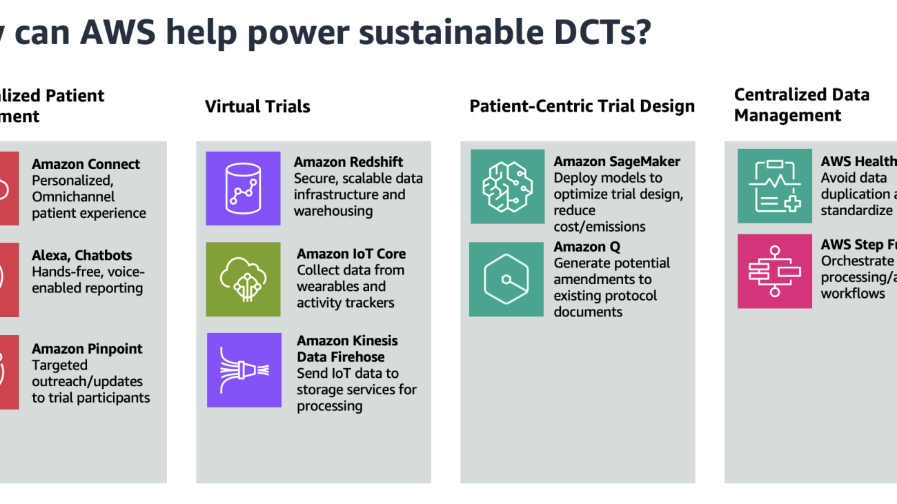
In this post, we provide sustainability-oriented guidance focused on four key areas: virtual trials, personalized patient engagement, patient-centric trial design, and centralized data management. The following figure showcases the AWS services that can help in these four areas.

Personalized remote patient engagement
The average dropout rate for clinical trials is 30%, so providing an omnichannel experience for subjects to interact with trial facilitators is imperative. Because decentralized clinical trials provide flexibility for patients to participate at home, the experience for patients to collect and report data should be seamless. One solution is to use voice applications to enable patient data reporting, using Amazon Alexa and Amazon Connect. For example, a patient can report symptoms to their Amazon Echo device, invoking an automated patient outreach scheduler using Amazon Connect.
Trial facilitators can also use Amazon Pinpoint to connect with customers through multiple channels. They can use Amazon Pinpoint to send medication reminders, automate surveys, or push other communications without the need for paper mail delivery.
Virtual trials
Decentralized clinical trials reduce emissions compared to regular clinical trials by eliminating the need for travel and physical infrastructure. Instead, a core component of decentralized clinical trials is a secure, scalable data infrastructure with strong data analytics capabilities. Amazon Redshift is a fully managed cloud data warehouse that trial scientists can use to perform analytics.
Clinical Research Organizations (CROs) and life sciences organizations can also use AWS for mobile device and wearable data capture. Patients, in the comfort of their own home, can collect data passively through wearables, activity trackers, and other smart devices. This data is streamed to AWS IoT Core, which can write data to Amazon Data Firehose in real time. This data can then be sent to services like Amazon Simple Storage Service (Amazon S3) and AWS Glue for data processing and insight extraction.
Patient-centric trial design
A key characteristic of decentralized clinical trials is patient-centric protocol design, which prioritizes the patients’ needs throughout the entire clinical trial process. This involves patient-reported outcomes and often implement flexible participation, which can complicate protocol development and necessitate more extensive regulatory documentation. This can add days or even weeks to the lifespan of a trial, leading to avoidable costs. Amazon SageMaker enables trial developers to build and train machine learning (ML) models that reduce the likelihood of protocol amendments and inconsistencies. Models can also be built to determine the appropriate sample size and recruitment timelines.
With SageMaker, you can optimize your ML environment for sustainability. Amazon SageMaker Debugger provides profiler capabilities to detect under-utilization of system resources, which helps right-size your environment and avoid unnecessary carbon emissions. Organizations can further reduce emissions by choosing deployment regions near renewable energy projects. Currently, there are 22 AWS data center regions where 100% of the electricity consumed is matched by renewable energy sources. Additionally, you can use Amazon Q, a generative AI-powered assistant, to surface and generate potential amendments to avoid expensive costs associated with protocol revisions.
Centralized data management
CROs and bio-pharmaceutical companies are striving to achieve end-to-end data linearity for all clinical trials within an organization. They want to see traceability across the board, while achieving data harmonization for regulatory clinical trial guardrails. The pipeline approach to data management in clinical trials has led to siloed, disconnected data across an organization, because separate storage is used for each trial. Decentralized clinical trials, however, often employ a singular data lake for all of an organization’s clinical trials.
With a centralized data lake, organizations can avoid the duplication of data across separate trial databases. This leads to savings in storage costs and computing resources, as well as a reduction in the environmental impact of maintaining multiple data silos. To build a data management platform, the process could begin with ingesting and normalizing clinical trial data using AWS HealthLake. HealthLake is designed to ingest data from various sources, such as electronic health records, medical imaging, and laboratory results, and automatically transform the data into the industry-standard FHIR format. This clinical voice application solution built entirely on AWS showcases the advantages of having a centralized location for clinical data, such as avoiding data drift and redundant storage.
With the normalized data now available in HealthLake, the next step would be to orchestrate the various data processing and analysis workflows using AWS Step Functions. You can use Step Functions to coordinate the integration of the HealthLake data into a centralized data lake, as well as invoke subsequent processing and analysis tasks. This could involve using serverless computing with AWS Lambda to perform event-driven data transformation, quality checks, and enrichment activities. By combining the power powerful data normalization capabilities of HealthLake and the orchestration features of Step Functions, the platform can provide a robust, scalable, and streamlined approach to managing decentralized clinical trial data within the organization.
Conclusion
In this post, we discussed the critical importance of sustainability in clinical trials. We provided an overview of the key distinctions between traditional centralized clinical trials and decentralized clinical trials. Importantly, we explored how AWS technologies can enable the development of more sustainable clinical trials, addressing the four main pillars that underpin a successful decentralized trial approach.
To learn more about how AWS can power sustainable clinical trials for your organization, reach out to your AWS Account representatives. For more information about optimizing your workloads for sustainability, see Optimizing Deep Learning Workloads for Sustainability on AWS.
References
[1] https://www.appliedclinicaltrialsonline.com/view/awareness-of-clinical-research-increases-among-underrepresented-groups [2] https://www.ncbi.nlm.nih.gov/pmc/articles/PMC1839193/ [3] https://pubmed.ncbi.nlm.nih.gov/15474134/ [4] ClinicalTrials.gov and https://www.iqvia.com/insights/the-iqvia-institute/reports/the-global-use-of-medicines-2022 [5] https://aws.amazon.com/startups/learn/next-generation-data-management-for-clinical-trials-research-built-on-aws?lang=en-US#overview [6] https://pubmed.ncbi.nlm.nih.gov/39148198/About the Authors
 Sid Rampally is a Customer Solutions Manager at AWS driving GenAI acceleration for Life Sciences customers. He writes about topics relevant to his customers, focusing on data engineering and machine learning. In his spare time, Sid enjoys walking his dog in Central Park and playing hockey.
 Nina Chen is a Customer Solutions Manager at AWS specializing in leading software companies to leverage the power of the AWS cloud to accelerate their product innovation and growth. With over 4 years of experience working in the strategic Independent Software Vendor (ISV) vertical, Nina enjoys guiding ISV partners through their cloud transformation journeys, helping them optimize their cloud infrastructure, driving product innovation, and deliver exceptional customer experiences.


 Glen Ireland is a Senior Enterprise Account Engineer at AWS in the Worldwide Public Sector. Glen’s areas of focus include empowering customers interested in building generative AI solutions using Amazon Q.
 Julia Hu is a Specialist Solutions Architect who helps AWS customers and partners build generative AI solutions using Amazon Q Business on AWS. Julia has over 4 years of experience developing solutions for customers adopting AWS services on the forefront of cloud technology.


 David Gildea is the VP of Product for Generative AI at Druva. With over 20 years of experience in cloud automation and emerging technologies, David has led transformative projects in data management and cloud infrastructure. As the founder and former CEO of CloudRanger, he pioneered innovative solutions to optimize cloud operations, later leading to its acquisition by Druva. Currently, David leads the Labs team in the Office of the CTO, spearheading R&D into generative AI initiatives across the organization, including projects like Dru Copilot, Dru Investigate, and Amazon Q. His expertise spans technical research, commercial planning, and product development, making him a prominent figure in the field of cloud technology and generative AI.
 Tom Nijs is an experienced backend and AI engineer at Druva, passionate about both learning and sharing knowledge. With a focus on optimizing systems and using AI, he’s dedicated to helping teams and developers bring innovative solutions to life.
 Corvus Lee is a Senior GenAI Labs Solutions Architect at AWS. He is passionate about designing and developing prototypes that use generative AI to solve customer problems. He also keeps up with the latest developments in generative AI and retrieval techniques by applying them to real-world scenarios.
 Fahad Ahmed is a Senior Solutions Architect at AWS and assists financial services customers. He has over 17 years of experience building and designing software applications. He recently found a new passion of making AI services accessible to the masses.


 Vineet Kachhawaha is a Sr. Solutions Architect at AWS focusing on AI/ML and generative AI. He co-leads the AWS for Legal Tech team within AWS. He is passionate about working with enterprise customers and partners to design, deploy, and scale AI/ML applications to derive business value.


 Sundar Raghavan is an AI/ML Specialist Solutions Architect at AWS, helping customers leverage SageMaker and Bedrock to build scalable and cost-efficient pipelines for computer vision applications, natural language processing, and generative AI. In his free time, Sundar loves exploring new places, sampling local eateries and embracing the great outdoors.
 Alan Ismaiel is a software engineer at AWS based in New York City. He focuses on building and maintaining scalable AI/ML products, like Amazon SageMaker Ground Truth and Amazon Bedrock Model Evaluation. Outside of work, Alan is learning how to play pickleball, with mixed results.
 Yinan Lang is a software engineer at AWS GroundTruth. He worked on GroundTruth, MechanicalTurk and Bedrock infrastructure, as well as customer facing projects for GroundTruth Plus. He also focuses on product security and worked on fixing risks and creating security tests. In leisure time, he is an audiophile and particularly loves to practice keyboard compositions by Bach.
 George King is a summer 2024 intern at Amazon AI. He studies Computer Science and Math at the University of Washington and is currently between his second and third year. George loves being outdoors, playing games (chess and all kinds of card games), and exploring Seattle, where he has lived his entire life.


 Jundong Qiao is a Machine Learning Engineer at AWS Professional Service, where he specializes in implementing and enhancing AI/ML capabilities across various sectors. His expertise encompasses building next-generation AI solutions, including chatbots and predictive models that drive efficiency and innovation.
 Michael Massey is a Cloud Application Architect at Amazon Web Services. He helps AWS customers achieve their goals by building highly-available and highly-scalable solutions on the AWS Cloud.
 Praveen Kumar Jeyarajan is a Principal DevOps Consultant at AWS, supporting Enterprise customers and their journey to the cloud. He has 13+ years of DevOps experience and is skilled in solving myriad technical challenges using the latest technologies. He holds a Masters degree in Software Engineering. Outside of work, he enjoys watching movies and playing tennis.


 Priti Aryamane is a Specialty Consultant at AWS Professional Services. With over 15 years of experience in contact centers and telecommunications, Priti specializes in helping customers achieve their desired business outcomes with customer experience on AWS using Amazon Lex, Amazon Connect, and generative AI features.
 Sanjeet Sanda is a Specialty Consultant at AWS Professional Services with over 20 years of experience in telecommunications, contact center technology, and customer experience. He specializes in designing and delivering customer-centric solutions with a focus on integrating and adapting existing enterprise call centers into Amazon Connect and Amazon Lex environments. Sanjeet is passionate about streamlining adoption processes by using automation wherever possible. Outside of work, Sanjeet enjoys hanging out with his family, having barbecues, and going to the beach.
 Yogesh Khemka is a Senior Software Development Engineer at AWS, where he works on large language models and natural language processing. He focuses on building systems and tooling for scalable distributed deep learning training and real-time inference.


 Kara Yang is a Data Scientist at AWS Professional Services in the San Francisco Bay Area, with extensive experience in AI/ML. She specializes in leveraging cloud computing, machine learning, and Generative AI to help customers address complex business challenges across various industries. Kara is passionate about innovation and continuous learning.
 Farshad Harirchi is a Principal Data Scientist at AWS Professional Services. He helps customers across industries, from retail to industrial and financial services, with the design and development of generative AI and machine learning solutions. Farshad brings extensive experience in the entire machine learning and MLOps stack. Outside of work, he enjoys traveling, playing outdoor sports, and exploring board games.
 James Poquiz is a Data Scientist with AWS Professional Services based in Orange County, California. He has a BS in Computer Science from the University of California, Irvine and has several years of experience working in the data domain having played many different roles. Today he works on implementing and deploying scalable ML solutions to achieve business outcomes for AWS clients.

 Ishan Singh is a Generative AI Data Scientist at Amazon Web Services, where he helps customers build innovative and responsible generative AI solutions and products. With a strong background in AI/ML, Ishan specializes in building Generative AI solutions that drive business value. Outside of work, he enjoys playing volleyball, exploring local bike trails, and spending time with his wife and dog, Beau.
 Chris Pecora is a Generative AI Data Scientist at Amazon Web Services. He is passionate about building innovative products and solutions while also focused on customer-obsessed science. When not running experiments and keeping up with the latest developments in generative AI, he loves spending time with his kids.
 Yanyan Zhang is a Senior Generative AI Data Scientist at Amazon Web Services, where she has been working on cutting-edge AI/ML technologies as a Generative AI Specialist, helping customers use generative AI to achieve their desired outcomes. Yanyan graduated from Texas A&M University with a PhD in Electrical Engineering. Outside of work, she loves traveling, working out, and exploring new things.
 Mani Khanuja is a Tech Lead – Generative AI Specialists, author of the book Applied Machine Learning and High Performance Computing on AWS, and a member of the Board of Directors for Women in Manufacturing Education Foundation Board. She leads machine learning projects in various domains such as computer vision, natural language processing, and generative AI. She speaks at internal and external conferences such AWS re:Invent, Women in Manufacturing West, YouTube webinars, and GHC 23. In her free time, she likes to go for long runs along the beach.