Generative AI models have seen tremendous growth, offering cutting-edge solutions for text generation, summarization, code generation, and question answering. Despite their versatility, these models often struggle when applied to niche or domain-specific tasks because their pre-training is typically based on large, generalized datasets. To address these gaps and maximize their utility in specialized scenarios, fine-tuning with domain-specific data is essential to boost accuracy and relevance.
Meta’s newly launched Llama 3.2 series sets a new benchmark in generative AI with its advanced multimodal capabilities and optimized performance across diverse hardware platforms. The collection spans lightweight models like Llama-3.2-1B and Llama-3.2-3B, which support up to 128,000 tokens of context and are tailored for edge devices. These models are ideal for on-device applications such as real-time summarization, instruction following, and multilingual text generation. On the other end of the spectrum, the larger Llama-3.2-11B and Llama-3.2-90B models offer powerful vision-enabled capabilities for tasks such as image understanding, document analysis, and visual grounding. This allows for sophisticated use cases like generating captions for images, interpreting complex graphs, and reasoning over visual data. For instance, the Meta Llama 3.2 models can analyze sales data presented in a graph to provide actionable insights or locate specific objects on a map using natural language instructions.
In this post, we demonstrate how to fine-tune Meta’s latest Llama 3.2 text generation models, Llama 3.2 1B and 3B, using Amazon SageMaker JumpStart for domain-specific applications. By using the pre-built solutions available in SageMaker JumpStart and the customizable Meta Llama 3.2 models, you can unlock the models’ enhanced reasoning, code generation, and instruction-following capabilities to tailor them for your unique use cases. Whether you’re working in finance, healthcare, or any other specialized field, fine-tuning these models will allow you to bridge the gap between general AI capabilities and domain-specific expertise.
Solution overview
SageMaker JumpStart is a robust feature within the SageMaker machine learning (ML) environment, offering practitioners a comprehensive hub of publicly available and proprietary foundation models (FMs). This managed service accelerates the ML development process by providing access to a growing list of cutting-edge models from leading model hubs and providers. You can quickly evaluate, compare, and select FMs based on predefined quality and responsibility metrics for tasks such as article summarization and image generation.
SageMaker JumpStart allows for full customization of pre-trained models to suit specific use cases using your own data. Deployment to production environments is streamlined through the user interface or SDK, enabling rapid integration into applications. The platform also supports organizational collaboration by allowing the sharing of artifacts, including models and notebooks, to expedite model building and deployment. Administrators can manage the visibility of models within the organization, enhancing governance and security.
Furthermore, SageMaker JumpStart enables practitioners to deploy models to dedicated SageMaker instances within a network-isolated environment, maintaining compliance and data protection. By using the robust training and deployment capabilities available in SageMaker, you can customize and scale models to meet diverse ML requirements efficiently.
Prerequisites
To try out this solution using SageMaker JumpStart, you’ll need the following prerequisites:
Fine-tune Meta Llama 3.2 text generation models
In this section, we demonstrate how to fine-tune Meta Llama 3.2 text generation models. We will first look at the approach of fine-tuning using the SageMaker Studio UI without having to write any code. We then also cover how to fine-tune the model using SageMaker Python SDK.
No-code fine-tuning using the SageMaker Studio UI
SageMaker JumpStart provides access to publicly available and proprietary FMs from third-party and proprietary providers. Data scientists and developers can quickly prototype and experiment with various ML use cases, accelerating the development and deployment of ML applications. It helps reduce the time and effort required to build ML models from scratch, allowing teams to focus on fine-tuning and customizing the models for their specific use cases. These models are released under different licenses designated by their respective sources. It’s essential to review and adhere to the applicable license terms before downloading or using these models to make sure they’re suitable for your intended use case.
You can access the Meta Llama 3.2 FMs through SageMaker JumpStart in the SageMaker Studio UI and the SageMaker Python SDK. In this section, we cover how to discover these models in SageMaker Studio.
SageMaker Studio is an IDE that offers a web-based visual interface for performing the ML development steps, from data preparation to model building, training, and deployment. For instructions on getting started and setting up SageMaker Studio, refer to Amazon SageMaker Studio.
- In SageMaker Studio, access SageMaker JumpStart by choosing JumpStart in the navigation pane.
 You’re presented with the list of public models offered by SageMaker, where you can explore other models from other providers.
- To start using the Meta Llama 3.2 models, under Providers, choose Meta.
 You’re presented with a list of the models available.
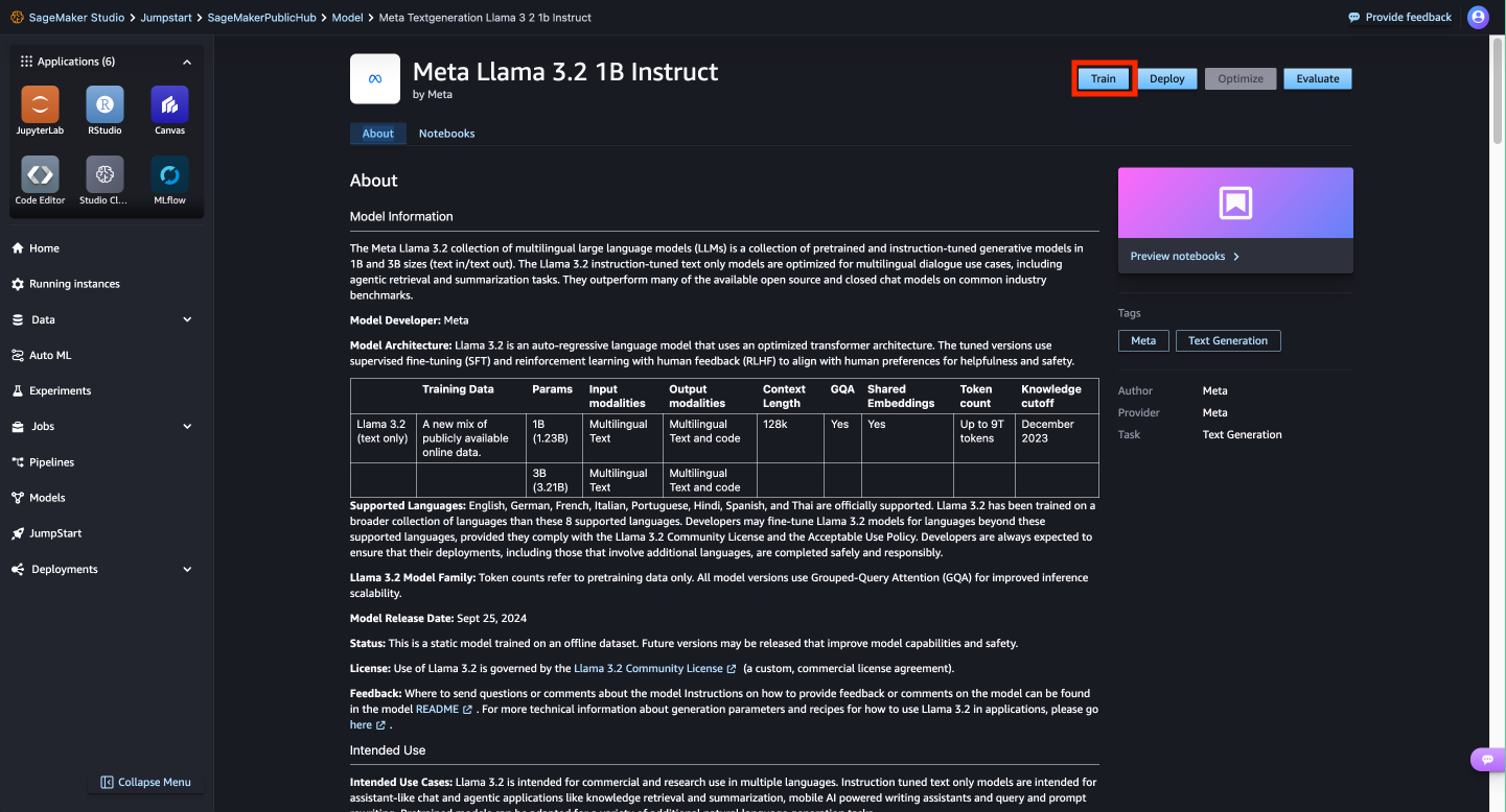
- Choose the Meta Llama 3.2 1B Instruct model.
 Here you can view the model details, as well as train, deploy, optimize, and evaluate the model.
- For this demonstration, we choose Train.
- On this page, you can point to the Amazon Simple Storage Service (Amazon S3) bucket containing the training and validation datasets for fine-tuning.
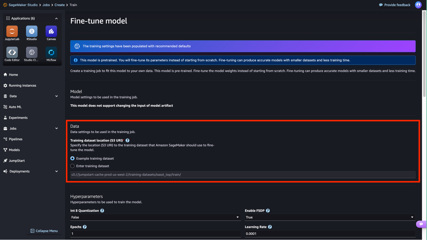
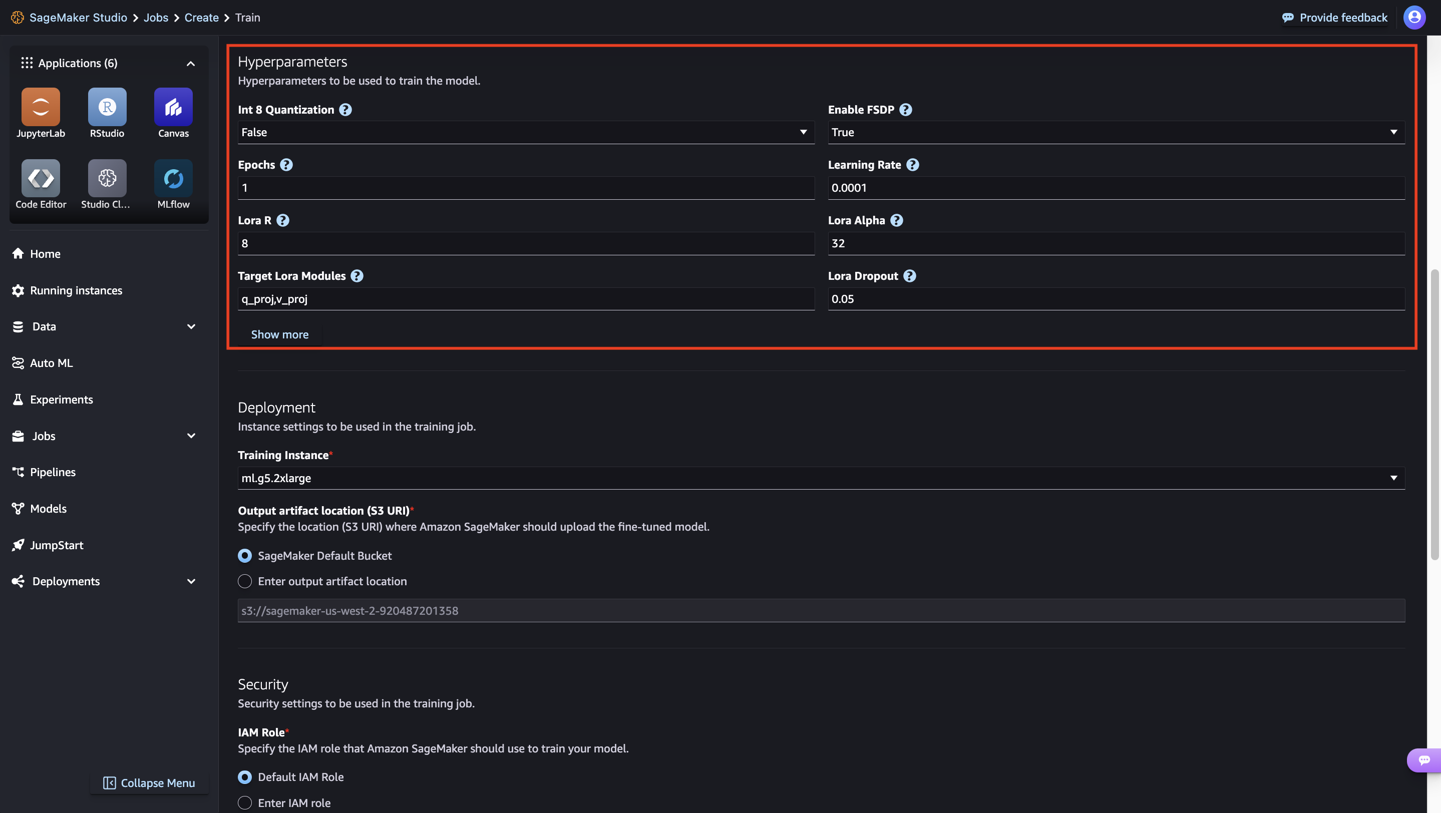
- In addition, you can configure deployment configuration, hyperparameters, and security settings for fine-tuning.
- Choose Submit to start the training job on a SageMaker ML instance.
- Accept the Llama 3.2 Community License Agreement to initiate the fine-tuning process.

Deploy the model
After the model is fine-tuned, you can deploy it using the model page on SageMaker JumpStart. The option to deploy the fine-tuned model will appear when fine-tuning is finished, as shown in the following screenshot.
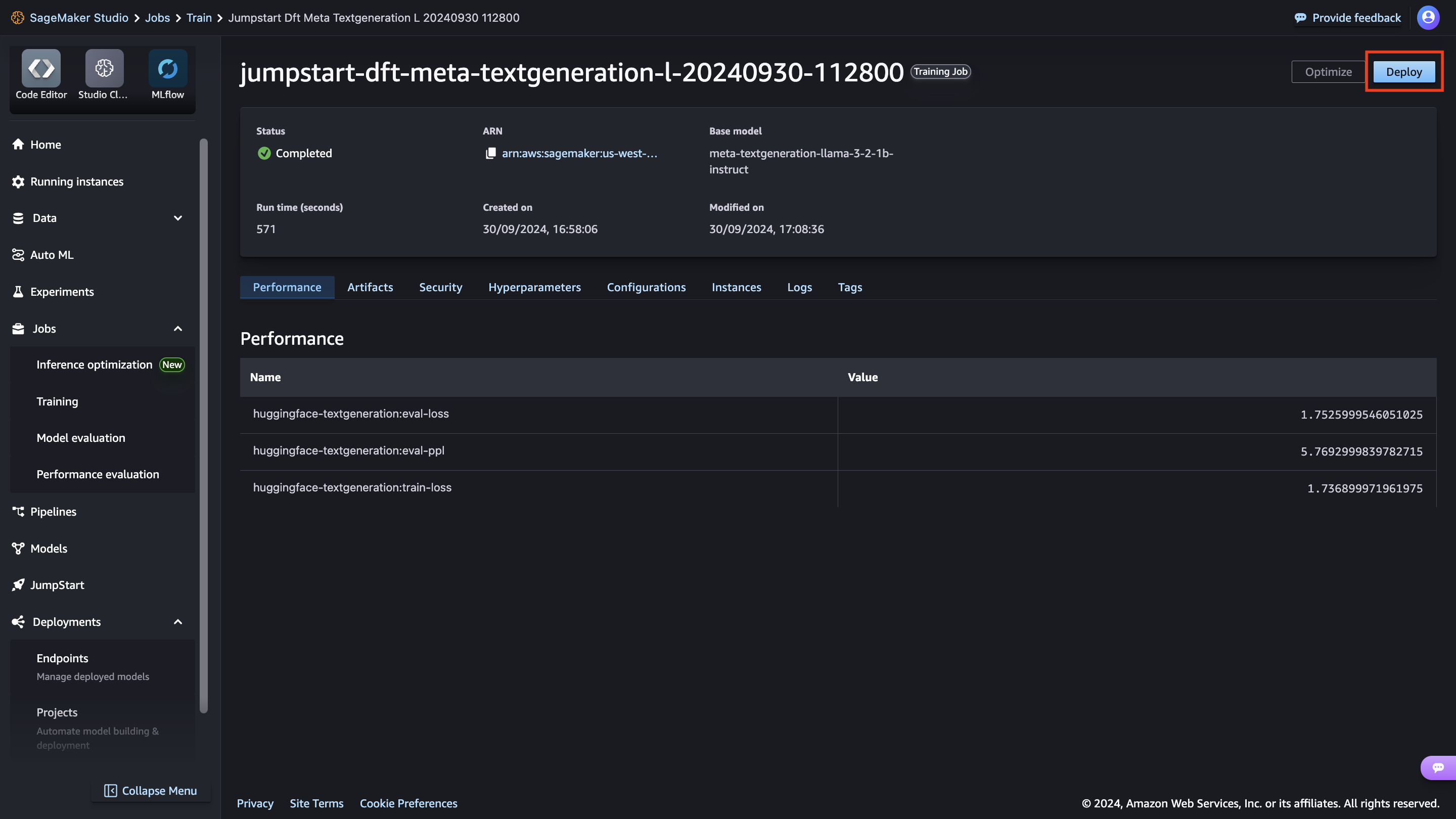
You can also deploy the model from this view. You can configure endpoint settings such as the instance type, number of instances, and endpoint name. You will need to accept the End User License Agreement (EULA) before you can deploy the model.

Fine-tune using the SageMaker Python SDK
You can also fine-tune Meta Llama 3.2 models using the SageMaker Python SDK. A sample notebook with the full instructions can be found on GitHub. The following code example demonstrates how to fine-tune the Meta Llama 3.2 1B model:
import os
import boto3
from sagemaker.session import Session
from sagemaker.jumpstart.estimator import JumpStartEstimator

# To fine-tune the Llama 3.2 3B model available on JumpStart, please change model_id to `meta-textgeneration-llama-3-2-3b`.
model_id = "meta-textgeneration-llama-3-2-1b"
accept_eula = "true"
estimator = JumpStartEstimator(
    model_id=model_id, environment={"accept_eula": accept_eula}
)

# By default, instruction tuning is set to false. Thus, to use instruction tuning dataset you use instruction_tuned="True"
estimator.set_hyperparameters(instruction_tuned="True", epoch="5", max_input_length = "1024",)
estimator.fit({"training": train_data_location})
The code sets up a SageMaker JumpStart estimator for fine-tuning the Meta Llama 3.2 large language model (LLM) on a custom training dataset. It configures the estimator with the desired model ID, accepts the EULA, enables instruction tuning by setting instruction_tuned="True", sets the number of training epochs, and initiates the fine-tuning process.
When the fine-tuning job is complete, you can deploy the fine-tuned model directly from the estimator, as shown in the following code. As part of the deploy settings, you can define the instance type you want to deploy the model on. For the full list of deployment parameters, refer to the deploy parameters in the SageMaker SDK documentation.
finetuned_predictor = estimator.deploy(instance_type='ml.g5.xlarge')
After the endpoint is up and running, you can perform an inference request against it using the predictor object as follows:
prompt = "Your prompt goes here"
payload = {
        "inputs": prompt,
        "parameters": {"max_new_tokens": 256},
    }
response = finetuned_predictor.predict(payload)
response.get('generated_text')
For the full list of predictor parameters, refer to the predictor object in the SageMaker SDK documentation.
Fine-tuning technique
Language models such as Meta Llama are more than 10 GB or even 100 GB in size. Fine-tuning such large models requires instances with significantly higher CUDA memory. Furthermore, training these models can be very slow due to their size. Therefore, for efficient fine-tuning, we use the following optimizations:
- Low-Rank Adaptation (LoRA) – This is a type of parameter efficient fine-tuning (PEFT) for efficient fine-tuning of large models. In this method, we freeze the whole model and only add a small set of adjustable parameters or layers into the model. For instance, instead of training all 3 billion parameters for Meta Llama 3.2 3B, we can fine-tune less than 1% of the parameters. This helps significantly reduce the memory requirement because we only need to store gradients, optimizer states, and other training-related information for only 1% of the parameters. Furthermore, this helps reduce both training time and cost. For more details on this method, refer to LoRA: Low-Rank Adaptation of Large Language Models.
- Int8 quantization – Even with optimizations such as LoRA, models like Meta Llama 70B require significant computational resources for training. To reduce the memory footprint during training, we can employ Int8 quantization. Quantization typically reduces the precision of the floating-point data types. Although this decreases the memory required to store model weights, it can potentially degrade the performance due to loss of information. However, Int8 quantization utilizes only a quarter of the precision compared to full-precision training, but it doesn’t incur significant degradation in performance. Instead of simply dropping bits, Int8 quantization rounds the data from one type to another, preserving the essential information while optimizing memory usage. To learn about Int8 quantization, refer to int8(): 8-bit Matrix Multiplication for Transformers at Scale.
- Fully Sharded Data Parallel (FSDP) – This is a type of data parallel training algorithm that shards the model’s parameters across data parallel workers and can optionally offload part of the training computation to the CPUs. Although the parameters are sharded across different GPUs, computation of each microbatch is local to the GPU worker. It shards parameters more uniformly and achieves optimized performance through communication and computation overlapping during training.
The following table compares different methods with the two Meta Llama 3.2 models.
| Model |
JumpStart Model IDs |
Default Instance Type |
Supported Instances Types for Fine-Tuning |
| Meta Llama 3.2 1B |
meta-textgeneration-llama-3-2-1b
meta-textgeneration-llama-3-2-1b-instruct
|
ml.g5.2xlarge |
ml.g5.2xlarge
ml.g5.4xlarge
ml.g5.8xlarge
ml.g5.12xlarge
ml.p3dn.24xlarge
ml.g4dn.12xlarge
ml.p5.48xlarge
|
| Meta Llama 3.2 3B |
meta-textgeneration-llama-3-2-3b
meta-textgeneration-llama-3-2-3b-instruct
|
ml.g5.12xlarge |
ml.g5.12xlarge
ml.g5.24xlarge
ml.g5.48xlarge
ml.p3dn.24xlarge
ml.g4dn.12xlarge
ml.p5.48xlarge
|
Other instance types may also work for fine-tuning. When using p3 instances, training will be done with 32-bit precision because bfloat16 is not supported on these instances. Therefore, the training job would consume double the amount of CUDA memory when training on p3 instances compared to g5 instances.
Training dataset format
SageMaker JumpStart currently support datasets in both domain adaptation format and instruction tuning format. In this section, we specify an example dataset in both formats. For more details, refer to the Dataset formatting section in the appendix.
Domain adaption format
You can fine-tune the Meta Llama 3.2 text generation model on domain-specific datasets, enabling it to generate relevant text and tackle various natural language processing (NLP) tasks within a particular domain using few-shot prompting. This fine-tuning process involves providing the model with a dataset specific to the target domain. The dataset can be in various formats, such as CSV, JSON, or TXT files. For example, if you want to fine-tune the model for the domain of financial reports and filings, you could provide it with a text file containing SEC filings from a company like Amazon. The following is an excerpt from such a filing:
This report includes estimates, projections, statements relating to our
business plans, objectives, and expected operating results that are “forward-
looking statements” within the meaning of the Private Securities Litigation
Reform Act of 1995, Section 27A of the Securities Act of 1933, and Section 21E
of the Securities Exchange Act of 1934. Forward-looking statements may appear
throughout this report, including the following sections: “Business” (Part I,
Item 1 of this Form 10-K), “Risk Factors” (Part I, Item 1A of this Form 10-K),
and “Management’s Discussion and Analysis of Financial Condition and Results
of Operations” (Part II, Item 7 of this Form 10-K). These forward-looking
statements generally are identified by the words “believe,” “project,”
“expect,” “anticipate,” “estimate,” “intend,” “strategy,” “future,”
“opportunity,” “plan,” “may,” “should,” “will,” “would,” “will be,” “will
continue,” “will likely result,” and similar expressions.
Instruction tuning format
In instruction fine-tuning, the model is fine-tuned for a set of NLP tasks described using instructions. This helps improve the model’s performance for unseen tasks with zero-shot prompts. In instruction tuning dataset format, you specify the template.json file describing the input and the output formats and the train.jsonl file with the training data item in each line.
The template.json file always has the following JSON format:
{
  "prompt": "<<Prompt goes here along with question or context or instruction>>",
  "completion": "<<completion goes here depending on the activity, for ex: answer for Q&A or summary for Summarization task>>"
}
For instance, the following table shows the template.json and train.jsonl files for the Dolly and Dialogsum datasets.
| Dataset |
Use Case |
template.json |
train.jsonl |
| Dolly |
Question Answering |
{
“prompt”: “Below is an instruction that describes a task, paired with an input that provides further context. Write a response that appropriately completes the request.nn### Instruction:n{instruction}nn### Input:n{context}nn”,
“completion”: ” {response}”
}
|
{ “instruction”: “Who painted the Two Monkeys”, “context”: “Two Monkeys or Two Chained Monkeys is a 1562 painting by Dutch and Flemish Renaissance artist Pieter Bruegel the Elder. The work is now in the Gemäldegalerie (Painting Gallery) of the Berlin State Museums.”, “response”: “The two Monkeys or Two Chained Monkeys is a 1562 painting by Dutch and Flemish Renaissance artist Pieter Bruegel the Elder. The work is now in the Gemaeldegalerie (Painting Gallery) of the Berlin State Museums.” } |
| Dialogsum |
Text Summarization |
{
“prompt”: “Below is a Instruction that holds conversation which describes discussion between two people.Write a response that appropriately summarizes the conversation.nn### Instruction:n{dialogue}nn”,
“completion”: ” {summary}”
}
|
{ “dialogue”: “#Person1#: Where do these flower vases come from? n#Person2#: They are made a town nearby. The flower vases are made of porcelain and covered with tiny bamboo sticks. n#Person1#: Are they breakable? n#Person2#: No. They are not only ornmamental, but also useful. n#Person1#: No wonder it’s so expensive. “, “summary”: “#Person2# explains the flower vases’ materials and advantages and #Person1# understands why they’re expensive.” }
|
Supported hyperparameters for training
The fine-tuning process for Meta Llama 3.2 models allows you to customize various hyperparameters, each of which can influence factors such as memory consumption, training speed, and the performance of the fine-tuned model. At the time of writing this post, the following are the default hyperparameter values. For the most up-to-date information, refer to the SageMaker Studio console, because these values may be subject to change.
- int8_quantization – If
True, the model is loaded with 8-bit precision for training. Default for Meta Llama 3.2 1B and Meta Llama 3.2 3B is False.
- enable_fsdp – If
True, training uses FSDP. Default for Meta Llama 3.2 1B and Meta Llama 3.2 3B is True.
- epoch – The number of passes that the fine-tuning algorithm takes through the training dataset. Must be an integer greater than 1. Default is 5.
- learning_rate – The rate at which the model weights are updated after working through each batch of training examples. Must be a positive float greater than 0. Default is 0.0001.
- lora_r – LoRA R dimension. Must be a positive integer. Default is 8.
- lora_alpha – LoRA Alpha. Must be a positive integer. Default is 32.
- target_modules – Target modules for LoRA fine-tuning. You can specify a subset of
[‘q_proj’,’v_proj’,’k_proj’,’o_proj’,’gate_proj’,’up_proj’,’down_proj’] modules as a string separated by a comma without any spaces. Default is q_proj,v_proj.
- lora_dropout – LoRA dropout. Must be a positive float between 0–1. Default is 0.05.
- instruction_tuned – Whether to instruction-train the model or not. At most, one of
instruction_tuned and chat_dataset can be True. Must be True or False. Default is False.
- chat_dataset – If
True, dataset is assumed to be in chat format. At most, one of instruction_tuned and chat_dataset can be True. Default is False.
- add_input_output_demarcation_key – For an instruction tuned dataset, if this is
True, a demarcation key ("### Response:n") is added between the prompt and completion before training. Default is True.
- per_device_train_batch_size – The batch size per GPU core/CPU for training. Default is 4.
- per_device_eval_batch_size – The batch size per GPU core/CPU for evaluation. Default is 1.
- max_train_samples – For debugging purposes or quicker training, truncate the number of training examples to this value. Value -1 means using all of the training samples. Must be a positive integer or -1. Default is -1.
- max_val_samples – For debugging purposes or quicker training, truncate the number of validation examples to this value. Value -1 means using all of the validation samples. Must be a positive integer or -1. Default is -1.
- seed – Random seed that will be set at the beginning of training. Default is 10.
- max_input_length – Maximum total input sequence length after tokenization. Sequences longer than this will be truncated. If -1, max_input_length is set to the minimum of 1024 and the maximum model length defined by the tokenizer. If set to a positive value,
max_input_length is set to the minimum of the provided value and the model_max_length defined by the tokenizer. Must be a positive integer or -1. Default is -1.
- validation_split_ratio – If validation channel is
None, ratio of train-validation split from the train data must be between 0–1. Default is 0.2.
- train_data_split_seed – If validation data is not present, this fixes the random splitting of the input training data to training and validation data used by the algorithm. Must be an integer. Default is 0.
- preprocessing_num_workers – The number of processes to use for preprocessing. If
None, the main process is used for preprocessing. Default is None.
Instance types and compatible hyperparameters
The memory requirement during fine-tuning may vary based on several factors:
- Model type – The 1B model has the smallest GPU memory requirement and the 3B model has a higher memory requirement
- Max input length – A higher value of input length leads to processing more tokens at a time and as such requires more CUDA memory
- Batch size – A larger batch size requires larger CUDA memory and therefore requires larger instance types
- Int8 quantization – If using Int8 quantization, the model is loaded into low precision mode and therefore requires less CUDA memory
To help you get started, we provide a set of combinations of different instance types, hyperparameters, and model types that can be successfully fine-tuned. You can select a configuration as per your requirements and availability of instance types. We fine-tune both two models on a variety of settings with three epochs on a subset of the Dolly dataset with summarization examples.
The results for fine-tuning the models are shown in the appendix at the end of this post. As we can see from these results, fine-tuning improves summarization compared to non-fine-tuned models.
Meta Llama 3.2 1B fine-tuning with various hyperparameters
The following table summarizes the different hyperparameters for fine-tuning Meta Llama 3.2 1B.
| Instance Type |
Max Input Length |
Per Device Training Batch Size |
Int8 Quantization |
Enable FSDP |
Time Taken (Minutes) |
| ml.g5.2xlarge |
1024 |
4 |
FALSE |
TRUE |
11.3 |
| ml.g5.2xlarge |
1024 |
8 |
FALSE |
TRUE |
11.12 |
| ml.g5.2xlarge |
1024 |
4 |
FALSE |
FALSE |
14.55 |
| ml.g5.2xlarge |
2048 |
4 |
FALSE |
TRUE |
10.95 |
| ml.g5.2xlarge |
1024 |
4 |
TRUE |
FALSE |
17.82 |
| ml.g5.2xlarge |
2048 |
4 |
TRUE |
FALSE |
17.4 |
| ml.g5.2xlarge |
1024 |
8 |
TRUE |
FALSE |
16.97 |
| ml.g5.4xlarge |
1024 |
8 |
FALSE |
TRUE |
11.28 |
| ml.g5.4xlarge |
1024 |
4 |
FALSE |
TRUE |
11.48 |
| ml.g5.4xlarge |
2048 |
4 |
FALSE |
TRUE |
11.27 |
| ml.g5.4xlarge |
1024 |
4 |
FALSE |
FALSE |
14.8 |
| ml.g5.4xlarge |
1024 |
4 |
TRUE |
FALSE |
17.38 |
| ml.g5.4xlarge |
1024 |
8 |
TRUE |
FALSE |
16.63 |
| ml.g5.4xlarge |
2048 |
4 |
TRUE |
FALSE |
16.8 |
| ml.g5.8xlarge |
1024 |
4 |
FALSE |
TRUE |
11.12 |
| ml.g5.8xlarge |
2048 |
4 |
FALSE |
TRUE |
10.87 |
| ml.g5.8xlarge |
1024 |
8 |
FALSE |
TRUE |
10.88 |
| ml.g5.8xlarge |
1024 |
4 |
FALSE |
FALSE |
14.47 |
| ml.g5.8xlarge |
1024 |
4 |
TRUE |
FALSE |
17.82 |
| ml.g5.8xlarge |
1024 |
8 |
TRUE |
FALSE |
17.13 |
| ml.g5.8xlarge |
2048 |
4 |
TRUE |
FALSE |
17.13 |
| ml.g5.12xlarge |
2048 |
4 |
FALSE |
FALSE |
14.72 |
| ml.g5.12xlarge |
1024 |
4 |
FALSE |
TRUE |
10.45 |
| ml.g5.12xlarge |
1024 |
8 |
TRUE |
FALSE |
17.23 |
| ml.g5.12xlarge |
1024 |
8 |
FALSE |
FALSE |
14.03 |
| ml.g5.12xlarge |
1024 |
4 |
FALSE |
FALSE |
14.22 |
| ml.g5.12xlarge |
1024 |
4 |
TRUE |
FALSE |
18.07 |
| ml.g5.12xlarge |
2048 |
4 |
TRUE |
FALSE |
18.15 |
| ml.g5.12xlarge |
2048 |
4 |
FALSE |
TRUE |
8.45 |
| ml.g5.12xlarge |
1024 |
8 |
FALSE |
TRUE |
8.87 |
| ml.g4dn.12xlarge |
1024 |
8 |
FALSE |
TRUE |
21.15 |
| ml.g4dn.12xlarge |
1024 |
4 |
TRUE |
FALSE |
35.12 |
| ml.g4dn.12xlarge |
1024 |
4 |
FALSE |
TRUE |
22.42 |
| ml.g4dn.12xlarge |
1024 |
4 |
FALSE |
FALSE |
34.62 |
| ml.g4dn.12xlarge |
2048 |
4 |
FALSE |
TRUE |
23.25 |
Meta Llama 3.2 3B fine-tuning with various hyper parameters
The following table summarizes the different hyperparameters for fine-tuning Meta Llama 3.2 3B.
| Instance Type |
Max Input Length |
Per Device Training Batch Size |
Int8 Quantization |
Enable FSDP |
Time Taken (Minutes) |
| ml.g5.12xlarge |
1024 |
8 |
TRUE |
FALSE |
29.18 |
| ml.g5.12xlarge |
2048 |
4 |
TRUE |
FALSE |
29.8 |
| ml.g5.12xlarge |
1024 |
4 |
FALSE |
FALSE |
26.2 |
| ml.g5.12xlarge |
1024 |
8 |
FALSE |
TRUE |
12.88 |
| ml.g5.12xlarge |
2048 |
4 |
FALSE |
TRUE |
11.8 |
| ml.g5.12xlarge |
1024 |
4 |
FALSE |
TRUE |
14.98 |
| ml.g5.12xlarge |
1024 |
4 |
TRUE |
FALSE |
30.05 |
| ml.g5.12xlarge |
1024 |
4 |
TRUE |
FALSE |
29.87 |
| ml.g5.24xlarge |
1024 |
4 |
FALSE |
FALSE |
25.97 |
| ml.g5.24xlarge |
1024 |
4 |
FALSE |
TRUE |
14.65 |
| ml.g5.24xlarge |
1024 |
4 |
TRUE |
FALSE |
29.32 |
| ml.g5.24xlarge |
2048 |
4 |
TRUE |
FALSE |
29.77 |
| ml.g5.24xlarge |
1024 |
8 |
TRUE |
FALSE |
28.78 |
| ml.g5.24xlarge |
2048 |
4 |
FALSE |
TRUE |
11.62 |
| ml.g5.24xlarge |
1024 |
8 |
FALSE |
TRUE |
12.38 |
| ml.g5.48xlarge |
1024 |
8 |
FALSE |
TRUE |
14.25 |
| ml.g5.48xlarge |
1024 |
4 |
FALSE |
FALSE |
26.2 |
| ml.g5.48xlarge |
2048 |
4 |
FALSE |
TRUE |
13.32 |
| ml.g5.48xlarge |
1024 |
4 |
FALSE |
TRUE |
16.73 |
| ml.g5.48xlarge |
1024 |
4 |
TRUE |
FALSE |
30.3 |
| ml.g5.48xlarge |
2048 |
4 |
FALSE |
FALSE |
28.7 |
| ml.g5.48xlarge |
1024 |
8 |
FALSE |
FALSE |
25.6 |
| ml.g5.48xlarge |
1024 |
8 |
TRUE |
FALSE |
29.33 |
| ml.g5.48xlarge |
2048 |
4 |
TRUE |
FALSE |
30.63 |
Recommendations on instance types and hyperparameters
When fine-tuning for the model’s accuracy, keep in mind the following:
- Larger models such as 3B provide better performance than 1B
- Performance without Int8 quantization is better than performance with Int8 quantization
Note the following training time and CUDA memory requirements:
- Setting
int8_quantization=True decreases the memory requirement.
- The combination of
per_device_train_batch_size, int8_quantization, and enable_fsdp settings affects the training times. When using a larger batch size with FSDP enabled, the training times are faster compared to using a larger batch size without FSDP.
- Decreasing
per_device_train_batch_size and max_input_length reduces the memory requirement and therefore can be run on smaller instances. However, setting very low values may increase the training time.
- If you’re not using Int8 quantization (
int8_quantization=False), use FSDP (enable_fsdp=True) for faster and efficient training.
When choosing the instance type, consider the following:
- At the time of writing this post, the G5 instances provided the most efficient training among the supported instance types. However, because AWS regularly updates and introduces new instance types, we recommend that you validate the recommended instance type for Meta Llama 3.2 fine-tuning in the SageMaker documentation or SageMaker console before proceeding.
- Training time largely depends on the amount of GPUs and the CUDA memory available. Therefore, training on instances with the same number of GPUs (for example, ml.g5.2xlarge and ml.g5.4xlarge) is roughly the same. Therefore, you can use the more cost-effective instance for training (ml.g5.2xlarge).
To learn about the cost of training per instance, refer to Amazon EC2 G5 Instances.
If your dataset is in instruction tuning format, where each sample consists of an instruction (input) and the desired model response (completion), and these input+completion sequences are short (for example, 50–100 words), using a high value for max_input_length can lead to poor performance. This is because the model may struggle to focus on the relevant information when dealing with a large number of padding tokens, and it can also lead to inefficient use of computational resources. The default value of -1 corresponds to a max_input_length of 1024 for Meta Llama models. We recommend setting max_input_length to a smaller value (for example, 200–400) when working with datasets containing shorter input+completion sequences to mitigate these issues and potentially improve the model’s performance and efficiency.
Lastly, due to the high demand of the G5 instances, you may experience unavailability of these instances in your AWS Region with the error “CapacityError: Unable to provision requested ML compute capacity. Please retry using a different ML instance type.” If you experience this error, retry the training job or try a different Region.
Issues when fine-tuning large models
In this section, we discuss two issues when fine-tuning very large models.
Disable output compression
By default, the output of a training job is a trained model that is compressed in a .tar.gz format before it’s uploaded to Amazon S3. However, for large models like the 70B model, this compression step can be time-consuming, taking more than 4 hours. To mitigate this delay, it’s recommended to use the disable_output_compression feature supported by the SageMaker training environment. When disable_output_compression is set to True, the model is uploaded without any compression, which can significantly reduce the time taken for large model artifacts to be uploaded to Amazon S3. The uncompressed model can then be used directly for deployment or further processing. The following code shows how to pass this parameter into the SageMaker JumpStart estimator:
estimator = JumpStartEstimator(
                                model_id=model_id,
                                environment={"accept_eula": "true"},
                                disable_output_compression=True
                                )
SageMaker Studio kernel timeout issue
The SageMaker Studio kernel is only used to initiate the training job, and its status doesn’t affect the ongoing training process. After the training job starts, the compute resources allocated for the job will continue running the training process, regardless of whether the SageMaker Studio kernel remains active or times out. If the kernel times out during the lengthy training process, you can still deploy the endpoint after training is complete using the training job name with the following code:
from sagemaker.jumpstart.estimator import JumpStartEstimator
training_job_name = <<<INSERT_TRAINING_JOB_NAME>>>

attached_estimator = JumpStartEstimator.attach(training_job_name, model_id)
attached_estimator.logs()
predictor = attached_estimator.deploy()
To find the training job name, navigate to the SageMaker console and under Training in the navigation pane, choose Training jobs. Identify the training job name and substitute it in the preceding code.
Clean up
To prevent incurring unnecessary charges, it’s recommended to clean up the deployed resources when you’re done using them. You can remove the deployed model with the following code:
predictor.delete_predictor()
Conclusion
As generative AI models continue to evolve, their effectiveness hinges on the ability to adapt and specialize for domain-specific applications. Meta’s Llama 3.2 series, with its innovative multimodal features and flexible deployment options, provides a powerful foundation for building tailored AI solutions. By fine-tuning these models using SageMaker JumpStart, organizations can transform generalized capabilities into highly specialized tools, enhancing precision and delivering meaningful results for complex, real-world problems. Whether you’re aiming to improve document analysis, automate visual interpretation, or generate domain-specific content, Meta Llama 3.2 models, fine-tuned to your needs, can bridge the gap between broad AI functionalities and targeted expertise, driving impactful outcomes in your field.
In this post, we discussed fine-tuning Meta Llama 3.2 text generation models using SageMaker JumpStart. We showed that you can use the SageMaker JumpStart console in SageMaker Studio or the SageMaker Python SDK to fine-tune and deploy these models. We also discussed the fine-tuning technique, instance types, and supported hyperparameters. In addition, we outlined recommendations for optimized training based on various tests we carried out.
As shown in the results of fine-tuning the models over two datasets, fine-tuning improves summarization compared to non-fine-tuned models.
As a next step, you can try fine-tuning these models on your own dataset using the code provided in the GitHub repository to test and benchmark the results for your use cases.
About the Authors
 Pavan Kumar Rao Navule is a Solutions Architect at Amazon Web Services, where he works with ISVs in India to help them innovate on the AWS platform. He is specialized in architecting AI/ML and generative AI services at AWS. Pavan is a published author for the book “Getting Started with V Programming.” In his free time, Pavan enjoys listening to the great magical voices of Sia and Rihanna.
 Jin Tan Ruan is a Prototyping Developer at AWS, part of the AWSI Strategic Prototyping and Customer Engineering (PACE) team, where he focuses on NLP and generative AI. With nine AWS certifications and a robust background in software development, Jin uses his expertise to help AWS strategic customers bring their AI/ML and generative AI projects to life. He holds a Master’s degree in Machine Learning and Software Engineering from Syracuse University. Outside of work, Jin is an avid gamer and a fan of horror films. You can find Jin on LinkedIn to learn more!
Appendix
In this section, we present the results for fine-tuning the Meta Llama 3.2 1B and 3B text generation models on different datasets. This section also covers the dataset formatting for domain adaptation and instruction fine-tuning techniques.
Results for fine-tuning the Meta Llama 3.2 1B text generation model on the Dolly dataset
| Inputs |
Ground Truth |
Response from non-finetuned model |
Response from fine-tuned model |
|
Below is an instruction that describes a task, paired with an input that provides further context. Write a response that appropriately completes the request.
### Instruction:
Write down some points on Yugoslav Cup using given paragraph as a base.
### Input:
The Yugoslav Cup was a tournament for which clubs from all tiers of the football pyramid were eligible to enter. In addition, amateur teams put together by individual Yugoslav People’s Army garrisons and various factories and industrial plants were also encouraged to enter, which meant that each cup edition could have several thousands of teams in its preliminary stages. These teams would play through a number of qualifying rounds before reaching the first round proper, in which they would be paired with top-flight teams.
### Response:
|
1. Clubs from all levels of the football pyramid were eligible to participate in the Yugoslav Cup.
2. Additionally, amateur teams assembled by numerous enterprises and industrial plants as well as individual Yugoslav People’s Army garrisons were encouraged to compete, which meant that each cup edition may include thousands of teams in its preliminary rounds.
3. Prior to the first round proper, where they would be partnered with top-flight teams, these teams would compete in a number of qualification rounds. |
The Yugoslav Cup was a tournament for which clubs from all tiers of the football pyramid were eligible to enter. In addition, amateur teams put together by individual Yugoslav People’s Army garrisons and various factories and industrial plants were also encouraged to enter, which meant that each cup edition could have several thousands of teams in its preliminary stages. These teams would play through a number of qualifying rounds before reaching the first round proper, in which they would be paired with top-flight teams.
### Input:
The
|
1. The Yugoslav Cup was a tournament for which clubs from all tiers of the football pyramid were eligible to enter. In addition, amateur teams put together by individual Yugoslav People’s Army garrisons and various factories and industrial plants were also encouraged to enter, which meant that each cup edition could have several thousands of teams in its preliminary stages. These teams would play through a number of qualifying rounds before reaching the first round proper, in which they would be paired with top-flight teams. |
|
Below is an instruction that describes a task, paired with an input that provides further context. Write a response that appropriately completes the request.
### Instruction:
What role did Danbury, Connecticut play in the American Revolution?
### Input:
During the Revolutionary War, Danbury was an important military supply depot for the Continental Army. Sybil Ludington, 16-year-old daughter of American Colonel Henry Ludington, is said to have made a 40-mile ride in the early hours of the night on April 26, 1777, to warn the people of Danbury and her father’s forces in Putnam County, New York, of the approach of British regulars, helping them muster in defense; these accounts, originating from the Ludington family, are questioned by modern scholars.
During the following day on April 26, 1777, the British, under Major General William Tryon, burned and sacked Danbury, but fatalities were limited due to Ludington’s warning. The central motto on the seal of the City of Danbury is Restituimus, (Latin for “We have restored”), a reference to the destruction caused by the Loyalist army troops. The American General David Wooster was mortally wounded at the Battle of Ridgefield by the British forces which had raided Danbury, but at the beginning of the battle, the Americans succeeded in driving the British forces down to Long Island Sound. Wooster is buried in Danbury’s Wooster Cemetery; the private Wooster School in Danbury also was named in his honor.
### Response:
|
Danbury, Connecticut served as an important military depot for the Continental Army during the revolutionary war. In April 26, 1777 the British Army attacked, burned and sacked the city, but the American troop were able to drive the British forces back to the Long Island sound. |
Danbury was an important military supply depot for the Continental Army. Sybil Ludington, 16-year-old daughter of American Colonel Henry Ludington, is said to have made a 40-mile ride in the early hours of the night on April 26, 1777, to warn the people of Danbury and her father’s forces in Putnam County, New York, of the approach of British regulars, helping them muster in defense; these accounts, originating from the Ludington family, |
During the Revolutionary War, Danbury was an important military supply depot for the Continental Army. Sybil Ludington, 16-year-old daughter of American Colonel Henry Ludington, is said to have made a 40-mile ride in the early hours of the night on April 26, 1777, to warn the people of Danbury and her father’s forces in Putnam County, New York, of the approach of British regulars, helping them muster in defense; these accounts, originating from |
|
Below is an instruction that describes a task, paired with an input that provides further context. Write a response that appropriately completes the request.
### Instruction:
Give me a bulleted list of the main responses to “Bad Blood” listed in this text, including whether they were positive or negative.
### Input:
“Bad Blood” is a song by American singer-songwriter Taylor Swift, taken from her fifth studio album 1989 (2014). Swift wrote the song with its producers Max Martin and Shellback. The album track is a pop song with stomping drums. A hip hop remix of “Bad Blood”, featuring American rapper Kendrick Lamar and additional production by Ilya, was released as the fourth single from 1989 on May 17, 2015, by Big Machine and Republic Records.
The lyrics are about feelings of betrayal by a close friend. Upon the album’s release, critics expressed mixed opinions about “Bad Blood”, with some complimenting Swift’s defiant attitude and dubbing it an album highlight, while others criticized its production and lyrics. The remixed single was praised for the reworked instrumentation and Lamar’s verses, which others considered to be out of place on a pop song. Media outlets speculated that American singer Katy Perry is the subject of the song. The remix received a Grammy nomination for Best Pop Duo/Group Performance.
“Bad Blood” was supported by a high-budget music video directed by Joseph Kahn and produced by Swift. It featured an ensemble cast consisting of many singers, actresses and fashion models, which received wide media coverage. Critics praised the video for its cinematic and futuristic visuals inspired by neo-noir styles. It won a Grammy Award for Best Music Video, and two MTV Video Music Awards for the Video of the Year and Best Collaboration. Commercially, “Bad Blood” reached number one in Australia, Canada, New Zealand, and Scotland, as well as the United States, where it topped the Billboard Hot 100, Adult Top 40 and Mainstream Top 40 charts. It has been certified triple platinum in Australia and Canada, and 6√ó platinum in the US.
### Response:
|
* positive about Taylor Swift’s defiant attitude
* negative about the song’s production and lyrics
* positive about the instrumentation and verses
* positive about the accompanying music video’s visuals
* positive in terms of topping several charts |
1. “Bad Blood” is a song by American singer-songwriter Taylor Swift, taken from her fifth studio album 1989 (2014). Swift wrote the song with its producers Max Martin and Shellback. The album track is a pop song with stomping drums. A hip hop remix of “Bad Blood”, featuring American rapper Kendrick Lamar and additional production by Ilya, was released as the fourth single from 1989 on May 17, 2015, by Big Machine and Republic |
1. The song is a pop song with stomping drums.
2. A hip hop remix of “Bad Blood”, featuring American rapper Kendrick Lamar and additional production by Ilya, was released as the fourth single from 1989 on May 17, 2015, by Big Machine and Republic Records.
3. The lyrics are about feelings of betrayal by a close friend.
4. Upon the album’s release, critics expressed mixed opinions about “Bad Blood”, with some complimenting Swift’s |
|
Below is an instruction that describes a task, paired with an input that provides further context. Write a response that appropriately completes the request.
### Instruction:
What are the highlights of the Apollo 11 mission?
### Input:
Apollo 11 (July 16‚Äì24, 1969) was the American spaceflight that first landed humans on the Moon. Commander Neil Armstrong and lunar module pilot Buzz Aldrin landed the Apollo Lunar Module Eagle on July 20, 1969, at 20:17 UTC, and Armstrong became the first person to step onto the Moon’s surface six hours and 39 minutes later, on July 21 at 02:56 UTC. Aldrin joined him 19 minutes later, and they spent about two and a quarter hours together exploring the site they had named Tranquility Base upon landing. Armstrong and Aldrin collected 47.5 pounds (21.5 kg) of lunar material to bring back to Earth as pilot Michael Collins flew the Command Module Columbia in lunar orbit, and were on the Moon’s surface for 21 hours, 36 minutes before lifting off to rejoin Columbia.
### Response:
|
Apollo 11 was the culmination of a multi year space race instigated by the Cold War, leading to the United States landing the first humans on the Moon. The mission had 3 personnel, required multiple years of preparation, and consisted of 8 key phases; launch, flight, lunar orbit, lunar descent, landing, lunar surface operations, lunar ascent, return, splashdown, and Quarantine. The Apollo 11 mission remains the most famous mission ever in the NASA program. The 3 astronauts were Michael Collins, Buzz Aldrin, and Neil Armstrong. |
The Apollo 11 mission was a historic event that changed the course of human history. It was the first time humans had landed on the Moon, and it was the first time humans had walked on the Moon. The mission was a success, and it was a major step forward in the exploration of space. The mission was also a major step forward in the exploration of the Moon, and it was a major step forward in the exploration of the Moon, and it was a major step forward in the exploration |
The Apollo 11 mission was the first manned mission to land humans on the Moon. The mission was led by Neil Armstrong and Buzz Aldrin, who landed the Apollo Lunar Module Eagle on July 20, 1969, at 20:17 UTC, and Armstrong became the first person to step onto the Moon’s surface six hours and 39 minutes later, on July 21 at 02:56 UTC. Aldrin joined him 19 minutes later, and they spent about two and a |
|
Below is an instruction that describes a task, paired with an input that provides further context. Write a response that appropriately completes the request.
### Instruction:
Extract the key elements from the paragraph about Apple and list them in bullet points
### Input:
Apple Inc. is an American multinational technology company headquartered in Cupertino, California. Apple is the largest technology company by revenue, totaling US$394.3 billion in 2022. As of March 2023, Apple is the world’s biggest company by market capitalization. As of June 2022, Apple is the fourth-largest personal computer vendor by unit sales and second-largest mobile phone manufacturer. It is one of the Big Five American information technology companies, alongside Alphabet (known for Google), Amazon, Meta (known for Facebook), and Microsoft.
Apple was founded as Apple Computer Company on April 1, 1976, by Steve Wozniak, Steve Jobs and Ronald Wayne to develop and sell Wozniak’s Apple I personal computer. It was incorporated by Jobs and Wozniak as Apple Computer, Inc. in 1977. The company’s second computer, the Apple II, became a best seller and one of the first mass-produced microcomputers. Apple went public in 1980 to instant financial success. The company developed computers featuring innovative graphical user interfaces, including the 1984 original Macintosh, announced that year in a critically acclaimed advertisement. By 1985, the high cost of its products, and power struggles between executives, caused problems. Wozniak stepped back from Apple amicably and pursued other ventures, while Jobs resigned bitterly and founded NeXT, taking some Apple employees with him.
As the market for personal computers expanded and evolved throughout the 1990s, Apple lost considerable market share to the lower-priced duopoly of the Microsoft Windows operating system on Intel-powered PC clones (also known as “Wintel”). In 1997, weeks away from bankruptcy, the company bought NeXT to resolve Apple’s unsuccessful operating system strategy and entice Jobs back to the company. Over the next decade, Jobs guided Apple back to profitability through a number of tactics including introducing the iMac, iPod, iPhone and iPad to critical acclaim, launching the “Think different” campaign and other memorable advertising campaigns, opening the Apple Store retail chain, and acquiring numerous companies to broaden the company’s product portfolio. When Jobs resigned in 2011 for health reasons, and died two months later, he was succeeded as CEO by Tim Cook.
Apple became the first publicly traded U.S. company to be valued at over $1 trillion in August 2018, then $2 trillion in August 2020, and $3 trillion in January 2022. As of January 2023, it was valued at around $2.2 trillion. The company receives criticism regarding the labor practices of its contractors, its environmental practices, and its business ethics, including anti-competitive practices and materials sourcing. Nevertheless, the company has a large following and enjoys a high level of brand loyalty. It is ranked as one of the world’s most valuable brands.
### Response:
|
1. Apple is an American multination technology company with revenues of over $394.3 billion as of 2022.
2. Apple is the 4th largest personal computer vendor by unit sales and the second-largest mobile phone manufacturer.
3. Apple was founded by Steve Jobs, Steve Wozniak, and Rold Wayne on April 1, 1976.
4. Steve Jobs guided Apple to profitability through a number of tactics including introducing the iMac, iPod, iPhone, and Ipad when it was facing losses.
5. Apple was the first publicly traded US company to be valued at over $1 trillion in August 2018.
|
1. Apple Inc. is an American multinational technology company headquartered in Cupertino, California. Apple is the largest technology company by revenue, totaling US$394.3 billion in 2022. As of March 2023, Apple is the world’s biggest company by market capitalization. As of June 2022, Apple is the fourth-largest personal computer vendor by unit sales and second-largest mobile phone manufacturer. It is one of the Big Five American information technology companies, alongside Alphabet (known for Google |
1. Apple Inc. is an American multinational technology company headquartered in Cupertino, California.
2. Apple is the largest technology company by revenue, totaling US$394.3 billion in 2022.
3. As of March 2023, Apple is the world’s biggest company by market capitalization.
4. As of June 2022, Apple is the fourth-largest personal computer vendor by unit sales and second-largest mobile phone manufacturer.
5. It is one of the Big Five American information |
Results for fine-tuning the Meta Llama 3.2 1B text generation model on the Dialogsum dataset
| Inputs |
Ground Truth |
Response from non-finetuned model |
Response from fine-tuned model |
|
Below is a Instruction that holds conversation which describes discussion between two people.Write a response that appropriately summarizes the conversation.
### Instruction:
#Person1#: Wow, Amy, look at that number.
#Person2#: What’s so great about it?
#Person1#: What do you mean? It’s a scrim.
#Person2#: Not to me, I wouldn’t be caught dead in that.
#Person1#: I love that kind of stuff.
#Person2#: Yeah, you seem to like those styles.
#Person1#: Sure do. I get a kick out of looking punk.
#Person2#: This one looks really expensive though.
#Person1#: I don’t care how much it costs. I’m rolling in it.
#Person2#: Lucky you! I can’t buy anything else. I’m flat broke.
#Person1#: I got a replace my party outfit, I trashed it last week.
#Person2#: Why did you drag me into this? I’ve spent a week salary.
#Person1#: Are you on the level? You’re the one who called me, remember?
#Person2#: Just joking, T. I’ve got some wonderful clothes. Let’s go and have a close look at your outfit.
### Response:
|
#Person1# trashed the party outfit so #Person1# needs a replacement. Amy jokes that she is broke. They then go to see the outfit. |
#Person1#: I’m not sure I like it. It’s a little too much.
#Person2#: I think it’s great. It’s a little bit of everything.
#Person1#: I’m not sure I like it. It’s a little too much.
#Person2#: I think it’s great. It’s a little bit of everything.
#Person1#: I’m not sure I like it. It’s a little too much.
#Person2#: I think it’s great. It’s a little bit of everything.
#Person1#: I’m not sure I like it. It’s a little too much.
#Person2#: I think it’s great. It’s a little bit of everything.
#Person1#: I’m not sure I like it. It’s a little too much.
#Person2#: I think it’s great. It’s a little bit of everything.
#Person1#: I’m not sure I like it. It’s a little too much.
#Person2#: I think it’s great. It’s a little bit of everything.
#Person1#: I’m not sure I like it. It’s a little too much.
#Person2#: I think it’s great. It’s a little bit of everything.
#Person1#: I’m not sure I like it. It’s a little too much.
#Person2#: I think it’s great. It’s a little bit of everything.
#Person1#: |
#Person1# and Amy are talking about the number of Amy’s outfit. #Person1# loves that kind of stuff and Amy is flat broke. |
|
Below is a Instruction that holds conversation which describes discussion between two people.Write a response that appropriately summarizes the conversation.
### Instruction:
#Person1#: So who does he think he is, anyway, I can’t believe the way that my boss has been ordering everyone around lately, I mean, it’s now like he is the CEO, or anything.
#Person2#: Um. . . Actually I am guessing you didn’t get the MEMO. Your boss was selected to fill the vacancy in the CEO slot. He actually is the CEO now, or will be, as soon as the official press releases and hoopla is done with.
#Person1#: Yikes! you are joking, right? I can’t believe it. No wonder he is so stressed and bossy lately. I thought he was just being ostentatious by giving orders to people and all the different departments. What big shoes to fill!
#Person2#: No kidding! When the last CEO left, we were worried about the future of the company.
#Person1#: What does a CEO do anyway? I know the CEO makes the most money in the company, but what does he actually do?
#Person2#: He is responsible to the board of directors for everything that happens in the company. He or she must give leadership to all company officers, as CEO is also responsible for providing the guidance of philosophy of the company, and acting as official representative, or face of the company.
#Person1#: Must be one smart guy.
### Response:
|
#Person1# complains about the style of CEO. #Person2# says that the boss is already a CEO candidate. #Person2# answers #Person1#’s question about the CEO’s function in a company. |
#Person1#: I think you are right. I mean, I can’t believe that my boss is the CEO. I mean, he is the CEO, but he is not the CEO. I mean, he is the CEO, but he is not the CEO. I mean, he is the CEO, but he is not the CEO. I mean, he is the CEO, but he is not the CEO. I mean, he is the CEO, but he is not the CEO. I mean, he is the CEO, but he is not the CEO. I mean, he is the CEO, but he is not the CEO. I mean, he is the CEO, but he is not the CEO. I mean, he is the CEO, but he is not the CEO. I mean, he is the CEO, but he is not the CEO. I mean, he is the CEO, but he is not the CEO. I mean, he is the CEO, but he is not the CEO. I mean, he is the CEO, but he is not the CEO. I mean, he is the CEO, but he is not the CEO. I mean, he is the CEO, but he is not the CEO. I mean, he is the CEO, but he is not the CEO. I mean, he is the CEO, but he is not the CEO. I mean, he is the CEO, but he is not the CEO. I mean, he is the |
#Person1# thinks #Person1#’s boss is being bossy lately. #Person2# tells #Person1# #Person2#’s boss is the CEO now. #Person1# thinks it’s a big shoes to fill. |
|
Below is a Instruction that holds conversation which describes discussion between two people.Write a response that appropriately summarizes the conversation.
### Instruction:
#Person1#: What does a housing go for in south mountain district?
#Person2#: It depends on the type of the house you’re looking for.
#Person1#: We’re looking for a three-bedroom home.
#Person2#: What’s your general price range?
#Person1#: Under 300, 000 RIB, we suppose.
#Person2#: Umm, I think I would be hard to find something in that range in this area. You know the environment in the south mountain district is the nicest.
#Person1#: What about a two-bedroom house?
#Person2#: A two-bedroom house in this area is generally around 250, 000 RIB.
#Person1#: I see.
#Person2#: I recommend you buy a two-bedroom house. It is very suitable for a couple, and some two-bedroom houses are large enough for a one-child family.
#Person1#: Okay, I will take it into consideration.
### Response:
|
#Person1# wants a three-bedroom home with a price under 300,000 RIB. #Person2# suggests buying a two-bedroom house for a one-child family with around 250, 000 RIB. |
#Person1#: What does a housing go for in south mountain district?
#Person2#: It depends on the type of the house you’re looking for.
#Person1#: We’re looking for a three-bedroom home.
#Person2#: What’s your general price range?
#Person1#: Under 300, 000 RIB, we suppose.
#Person2#: Umm, I think I would be hard to find something in that range in this area. You know the environment in the south mountain district is the nicest.
#Person1#: What about a two-bedroom house?
#Person2#: A two-bedroom house in this area is generally around 250, 000 RIB.
#Person1#: I see.
#Person2#: I recommend you buy a two-bedroom house. It is very suitable for a couple, and some two-bedroom houses are large enough for a one-child family.
#Person1#: Okay, I will take it into consideration. |
#Person1# and #Person2# are looking for a three-bedroom home. #Person2# recommends #Person1# to buy a two-bedroom house. |
|
Below is a Instruction that holds conversation which describes discussion between two people.Write a response that appropriately summarizes the conversation.
### Instruction:
#Person1#: Mr. Sharp, thank you for giving me this interview. So, my first question is, are you happy with your life?
#Person2#: Am I happy? You may know you are the first person to have asked me this question directly. The others dared not because they were afraid I might say yes. They wanted me to say no so that they could make up stories about me.
#Person1#: What kind of stories?
#Person2#: Brian Sharpe, author of over 100 historical novels, lives in a lonely house 30 miles away from Sydney. But is he happy?
#Person1#: Is that why you have refused many interviews?
#Person2#: I’m tired of being told that I must be unhappy because I’m rich and successful. I’m not unhappy.
#Person1#: Understood. And I’m wondering if you follow a similar pattern of writing.
#Person2#: I know what you mean. Do I write similar stories? I say no.
#Person1#: So, how do you create your heroes?
#Person2#: My heroes live? They think for themselves. All their stories are drawn from life, my life, my friends’ lives, including my friends in many books.
#Person1#: Sounds good to me.
### Response:
|
#Person1# interviews Mr. Sharp. Mr. Sharp tells #Person1# he’s happy and he doesn’t write similar stories. His stories are drawn from life. |
#Person1#: I’m glad you’re happy. I’m glad you’re not Brian Sharpe. I’m glad you’re not Brian Sharpe. I’m glad you’re not Brian Sharpe. I’m glad you’re not Brian Sharpe. I’m glad you’re not Brian Sharpe. I’m glad you’re not Brian Sharpe. I’m glad you’re not Brian Sharpe. I’m glad you’re not Brian Sharpe. I’m glad you’re not Brian Sharpe. I’m glad you’re not Brian Sharpe. I’m glad you’re not Brian Sharpe. I’m glad you’re not Brian Sharpe. I’m glad you’re not Brian Sharpe. I’m glad you’re not Brian Sharpe. I’m glad you’re not Brian Sharpe. I’m glad you’re not Brian Sharpe. I’m glad you’re not Brian Sharpe. I’m glad you’re not Brian Sharpe. I’m glad you’re not Brian Sharpe. I’m glad you’re not Brian Sharpe. I’m glad you’re not Brian Sharpe. I’m glad you’re not Brian Sharpe. I’m glad you’re not Brian Sharpe. I’m glad you’re not Brian Sharpe. I’m glad you’re not Brian Sharpe. I’m glad you’re not Brian Sharpe. I’m glad you’re not Brian Sharpe. I’m glad you’re not Brian Sharpe. I’m glad you’re not Brian Sharpe |
Mr. Sharp is happy with his life. He tells #Person1# he doesn’t follow a similar pattern of writing. He thinks for himself and all his stories are drawn from life. |
|
Below is a Instruction that holds conversation which describes discussion between two people.Write a response that appropriately summarizes the conversation.
### Instruction:
#Person1#: What’s the weather forecast for today?
#Person2#: Cloudy in the morning, overcast in the afternoon.
#Person1#: Any rain?
#Person2#: No, but I wouldn’t be surprised if it rained tomorrow.
#Person1#: I wouldn’t either. It’s been looking like rain for several days.
### Response:
|
#Person2# tells #Person1# the weather forecast for today. |
#Person1#: It’s been looking like rain for several days.
#Person2#: I wouldn’t be surprised if it rained tomorrow.
#Person1#: I wouldn’t either. It’s been looking like rain for several days.
#Person2#: It’s been looking like rain for several days.
#Person1#: It’s been looking like rain for several days.
#Person2#: I wouldn’t be surprised if it rained tomorrow.
#Person1#: I wouldn’t either. It’s been looking like rain for several days.
#Person2#: It’s been looking like rain for several days.
#Person1#: It’s been looking like rain for several days.
#Person2#: I wouldn’t be surprised if it rained tomorrow.
#Person1#: I wouldn’t either. It’s been looking like rain for several days.
#Person2#: It’s been looking like rain for several days.
#Person1#: It’s been looking like rain for several days.
#Person2#: I wouldn’t be surprised if it rained tomorrow.
#Person1#: I wouldn’t either. It’s been looking like rain for several days.
#Person2#: It’s been looking like rain for several days.
#Person1#: It’s been looking like rain for several days.
#Person2#: I wouldn’t be surprised if it rained tomorrow.
#Person1#: I wouldn’t either. It’s been looking like rain for several days.
#Person2#: |
#Person1# and #Person2# talk about the weather forecast. |
Results for fine-tuning the Meta Llama 3.2 3B text generation model on the Dolly dataset
| Inputs |
Ground Truth |
Response from non-finetuned model |
Response from fine-tuned model |
|
Below is an instruction that describes a task, paired with an input that provides further context. Write a response that appropriately completes the request.
### Instruction:
Highlight relevant facts related to Heidelberg
### Input:
Heidelberg (German: [Ààha… dléb…õ Åk] (listen); Palatine German: Heidlberg) is a city in the German state of Baden-W√ºrttemberg, situated on the river Neckar in south-west Germany. As of the 2016 census, its population was 159,914, of which roughly a quarter consisted of students. dléb…õ Åk] (listen); Palatine German: Heidlberg) is a city in the German state of Baden-W√ºrttemberg, situated on the river Neckar in south-west Germany. As of the 2016 census, its population was 159,914, of which roughly a quarter consisted of students.
Located about 78 km (48 mi) south of Frankfurt, Heidelberg is the fifth-largest city in Baden-Württemberg. Heidelberg is part of the densely populated Rhine-Neckar Metropolitan Region.
Heidelberg University, founded in 1386, is Germany’s oldest and one of Europe’s most reputable universities. Heidelberg is a scientific hub in Germany and home to several internationally renowned research facilities adjacent to its university, including the European Molecular Biology Laboratory and four Max Planck Institutes. The city has also been a hub for the arts, especially literature, throughout the centuries, and it was designated a “City of Literature” by the UNESCO Creative Cities Network.
Heidelberg was a seat of government of the former Electorate of the Palatinate and is a popular tourist destination due to its romantic cityscape, including Heidelberg Castle, the Philosophers’ Walk, and the Baroque old town.
### Response:
|
Heidelberg has the oldest University in Germany. The city is a scientific hub and home to several internationally renowned research facilities. It was designated a “City of Literature” by the UNESCO Creative Cities Network. |
Heidelberg is a city in the German state of Baden-Württemberg, situated on the river Neckar in south-west Germany. As of the 2016 census, its population was 159,914, of which roughly a quarter consisted of students. Located about 78 km (48 mi) south of Frankfurt, Heidelberg is the fifth-largest city in Baden-Württemberg. Heidelberg is part of the densely populated Rhine-Neckar Metropolitan Region. |
Heidelberg is a city in the German state of Baden-Württemberg, situated on the river Neckar in south-west Germany. As of the 2016 census, its population was 159,914, of which roughly a quarter consisted of students.
Located about 78 km (48 mi) south of Frankfurt, Heidelberg is the fifth-largest city in Baden-Württemberg. Heidelberg is part of the densely populated Rhine-Neckar Metropolitan Region.
|
|
Below is an instruction that describes a task, paired with an input that provides further context. Write a response that appropriately completes the request.
### Instruction:
What is the Indianapolis 500?
### Input:
The Indianapolis 500, formally known as the Indianapolis 500-Mile Race, and commonly called the Indy 500, is an annual automobile race held at Indianapolis Motor Speedway (IMS) in Speedway, Indiana, United States, an enclave suburb of Indianapolis. The event is traditionally held over Memorial Day weekend, usually the last weekend of May. It is contested as part of the IndyCar Series, the top level of American open-wheel car racing, a formula colloquially known as “Indy car racing”. The track itself is nicknamed the “Brickyard”, as the racing surface was paved in brick in the fall of 1909. One yard of brick remains exposed at the start/finish line. The event, billed as The Greatest Spectacle in Racing, is considered part of the Triple Crown of Motorsport along with the 24 Hours of Le Mans and the Monaco Grand Prix, with which it typically shares a date.
### Response:
|
The Indianapolis 500, formally known as the Indianapolis 500-Mile Race, and commonly called the Indy 500, is an annual automobile race held at Indianapolis Motor Speedway (IMS) in Speedway, Indiana, United States, an enclave suburb of Indianapolis. The event is traditionally held over Memorial Day weekend, usually the last weekend of May. It is contested as part of the IndyCar Series, the top level of American open-wheel car racing, a formula colloquially known as “Indy car racing”. The track itself is nicknamed the “Brickyard”, as the racing surface was paved in brick in the fall of 1909. One yard of brick remains exposed at the start/finish line. The event, billed as The Greatest Spectacle in Racing, is considered part of the Triple Crown of Motorsport along with the 24 Hours of Le Mans and the Monaco Grand Prix, with which it typically shares a date.
The inaugural race was held in 1911 and was won by Ray Harroun. The event celebrated its 100th anniversary in 2011, and the 100th running was held in 2016. The event was put on hiatus twice, from 1917 to 1918 due to World War I and from 1942 to 1945 due to World War II. In two different periods, the race was part of FIA World Championships; between 1925 and 1928, the World Manufacturers’ Championship and between 1950 and 1960, the World Drivers’ Championship.
Marcus Ericsson is the current champion. The most successful drivers are A. J. Foyt, Al Unser Sr., Rick Mears and Hélio Castroneves, each of whom has won the race four times. The active driver with the most victories is Hélio Castroneves. Rick Mears holds the record for most career pole positions with six. The most successful car owner is Roger Penske, owner of the Indianapolis Motor Speedway and Team Penske, which has 18 total wins and 18 poles. Penske also has five wins at the IndyCar Grand Prix, held on the combined road course.
The event is steeped in tradition, in pre-race ceremonies, post-race celebrations, and race procedure. The most noteworthy and most popular traditions are the 33-car field lining up three-wide for the start, the annual singing of the chorus of “Back Home Again in Indiana,” and the victory lane bottle of milk. Also unique is that qualifying requires the driver to complete four, rather than one, timed laps. Qualifying has a separate weekend. The official attendance is not disclosed by Speedway management, but the permanent seating capacity is upwards of 250,000, and infield patrons raise the race-day attendance to approximately 300,000.
|
The Indianapolis 500 is an annual automobile race held at Indianapolis Motor Speedway (IMS) in Speedway, Indiana, United States, an enclave suburb of Indianapolis. The event is traditionally held over Memorial Day weekend, usually the last weekend of May. It is contested as part of the IndyCar Series, the top level of American open-wheel car racing, a formula colloquially known as “Indy car racing”. The track itself is nicknamed the “Brickyard”, as the racing surface was paved in |
The Indianapolis 500 is an annual automobile race held at Indianapolis Motor Speedway (IMS) in Speedway, Indiana, United States, an enclave suburb of Indianapolis. The event is traditionally held over Memorial Day weekend, usually the last weekend of May. It is contested as part of the IndyCar Series, the top level of American open-wheel car racing, a formula colloquially known as “Indy car racing”. The track itself is nicknamed the “Brickyard”, as the racing surface was paved in |
|
Below is an instruction that describes a task, paired with an input that provides further context. Write a response that appropriately completes the request.
### Instruction:
What are some interesting facts about Nelson Mandel Boulevard described on this paragraph?
### Input:
Nelson Mandela Boulevard (Persian: بلوار نلسون ماندلا) (old name: Jordan Street and Africa Boulevard) still known as Jordan is an affluent and upper-class district in northern Tehran, and some people draw similarities between Jordan District as being much alike Kensington District in London, UK as the area is a mixture of residential and commercial locale, filled with the homes and businesses of many politicians, diplomats, expatriates, and artists. Before the Iranian Revolution in 1979 it was called Jordan street, named after the American presbyterian missionary Samuel M. Jordan and used to be one of the most popular avenue in Tehran, Iran. Renamed Nelson Mandela Boulevard in recent years, it is amongst the most famous streets in north Tehran after Valiasr Street which is the longest conventional street in the Middle East, spanning a south–north axis. It is also famous for being one of the liveliest streets of Tehran, experiencing regular traffic jams even at 2:00A.M during Summer.
### Response:
|
It holds a mixture of residential and commercial locale from upper-class citizens, like politicians, diplomats, expatriates and artists. It used to be called Jordan street before the Iranian revolution. It’s amongst the most famous streets of Tehran, experiencing regular traffic jams even at 2:00 AM during Summer. |
Nelson Mandela Boulevard is a street in Tehran, Iran. It is one of the most famous streets in north Tehran after Valiasr Street which is the longest conventional street in the Middle East, spanning a south–north axis. It is also famous for being one of the liveliest streets of Tehran, experiencing regular traffic jams even at 2:00A.M during Summer. The street is named after the South African anti-apartheid revolutionary and former President of South Africa, Nelson Mandela. |
1. Nelson Mandela Boulevard is a street in northern Tehran, Iran.
2. It was named after the American presbyterian missionary Samuel M. Jordan.
3. It was renamed Nelson Mandela Boulevard in recent years.
4. It is amongst the most famous streets in north Tehran.
5. It is also famous for being one of the liveliest streets of Tehran. |
|
Below is an instruction that describes a task, paired with an input that provides further context. Write a response that appropriately completes the request.
### Instruction:
What are the Wimbledon Championships?
### Input:
The Wimbledon Championships, commonly known simply as Wimbledon, is the oldest tennis tournament in the world and is widely regarded as the most prestigious. It has been held at the All England Club in Wimbledon, London, since 1877 and is played on outdoor grass courts, with retractable roofs over the two main courts since 2019.
### Response:
|
The Wimbledon Championships, commonly known simply as Wimbledon, is the oldest tennis tournament in the world and is widely regarded as the most prestigious. It has been held at the All England Club in Wimbledon, London, since 1877 and is played on outdoor grass courts, with retractable roofs over the two main courts since 2019.
Wimbledon is one of the four Grand Slam tennis tournaments, the others being the Australian Open, the French Open, and the US Open. Wimbledon is the only major still played on grass, the traditional tennis playing surface. Also, it is the only Grand Slam that retains a night-time curfew, though matches can now continue until 11.00 pm under the lights.
The tournament traditionally takes place over two weeks in late June and early July, starting on the last Monday in June and culminating with the Ladies’ and Gentlemen’s Singles Finals, scheduled for the Saturday and Sunday at the end of the second week. Five major events are held each year, with additional junior and invitational competitions also taking place. In 2009, Wimbledon’s Centre Court was fitted with a retractable roof to lessen the loss of playing time due to rain. A roof was operational over No. 1 Court from 2019, when a number of other improvements were made, including adding cushioned seating, a table and 10 independently operable cameras per court to capture the games.
Wimbledon traditions include a strict all-white dress code for competitors, and royal patronage. Strawberries and cream are traditionally consumed at the tournament. Unlike other tournaments, advertising is minimal and low key from official suppliers such as Slazenger and Rolex. The relationship with Slazenger is the world’s longest-running sporting sponsorship, providing balls for the tournament since 1902.
Due to the COVID-19 pandemic, 2020 Wimbledon was cancelled, the first cancellation of the tournament since World War II. The rescheduled 134th edition was staged from 28 June 2021 to 11 July 2021, following from the 2020 cancellation. The 135th edition was played between 27 June 2022 and 10 July 2022, and regularly scheduled play occurred on the middle Sunday for the first time. It marks the centenary of the inaugural championships staged at the Centre Court. The ATP, ITF, and WTA did not award ranking points for the 2022 tournament, due to controversy over the tournament excluding players representing Russia and Belarus.
The 2023 Wimbledon Championships will be the 136th staging and will run from 3 July 2023 to 16 July 2023 and it will be the first event of King Charles III since the death of the former patron, Queen Elizabeth II on 8 September 2022.
|
The Wimbledon Championships, commonly known simply as Wimbledon, is the oldest tennis tournament in the world and is widely regarded as the most prestigious. It has been held at the All England Club in Wimbledon, London, since 1877 and is played on outdoor grass courts, with retractable roofs over the two main courts since 2019. The tournament consists of five men’s singles events and five women’s singles events. The men’s singles is the most prestigious of the five men’s singles events, and |
The Wimbledon Championships, commonly known simply as Wimbledon, is the oldest tennis tournament in the world and is widely regarded as the most prestigious. It has been held at the All England Club in Wimbledon, London, since 1877 and is played on outdoor grass courts, with retractable roofs over the two main courts since 2019. |
|
Below is an instruction that describes a task, paired with an input that provides further context. Write a response that appropriately completes the request.
### Instruction:
What are the different type of coats of dogs?
### Input:
The coats of domestic dogs are of two varieties: “double” being familiar with dogs (as well as wolves) originating from colder climates, made up of a coarse guard hair and a soft down hair, or “single”, with the topcoat only. Breeds may have an occasional “blaze”, stripe, or “star” of white fur on their chest or underside. Premature graying can occur in dogs from as early as one year of age; this is associated with impulsive behaviors, anxiety behaviors, fear of noise, and fear of unfamiliar people or animals.
### Response:
|
The coat of a dog varies depending on its breed. Typically a dog could have either a “double” coat or a “single” coat. “Double” coats are originated from breeds that live in colder climates. This type of coat consist of a coarse guard hair and a soft down hair. Dogs with “single” coat only has the topcoat. |
The coats of domestic dogs are of two varieties: “double” being familiar with dogs (as well as wolves) originating from colder climates, made up of a coarse guard hair and a soft down hair, or “single”, with the topcoat only. Breeds may have an occasional “blaze”, stripe, or “star” of white fur on their chest or underside. Premature graying can occur in dogs from as early as one year of age; this is associated with impulsive behaviors |
There are two types of coats of dogs: double and single. Double coats are made up of a coarse guard hair and a soft down hair. Single coats only have a topcoat. |
Results for fine-tuning the Meta Llama 3.2 3B text generation model on the Dialogsum dataset
| Inputs |
Ground Truth |
Response from non-finetuned model |
Response from fine-tuned model |
|
Below is a Instruction that holds conversation which describes discussion between two people.Write a response that appropriately summarizes the conversation.
### Instruction:
#Person1#: Farmington? Would you take a look at these catalogue ads that Roger did? I don’t think we can use them.
#Person2#: Hmm. I see what you mean. Have you spoken with Roger? He usually does better work than this.
#Person1#: I know, Mr. Farmington. But, I’m not sure that I should bring this up with him. I think it would be better if you spoke to him.
#Person2#: All right. Leave these ads with me. I’ll speak to him this morning.
### Response:
|
#Person1# and Farmington feel dissatisfied with the ads that Roger did. Farmington will speak to Roger. |
The conversation between Person1 and Person2 revolves around a set of catalogue ads that Person1 has found. Person1 expresses their concerns about the quality of the ads, suggesting that they may not be suitable for use. Person2 agrees with Person1’s concerns and suggests that they should speak with Roger, the person responsible for creating the ads. Person2 offers to take a look at the ads and speak with Roger in the morning, indicating that they will address the issue. The conversation is focused on finding a solution to the problem with the catalogue ads. |
#Person1# thinks the catalogue ads are not good. Mr. Farmington will speak to Roger. |
|
Below is a Instruction that holds conversation which describes discussion between two people.Write a response that appropriately summarizes the conversation.
### Instruction:
#Person1#: May I help you?
#Person2#: My daughter. She is missing. I don’t know where she is.
#Person1#: What dose she look like?
#Person2#: She has blond hair and blue eyes.
#Person1#: What was she wearing?
#Person2#: She has a yellow dress on and red sneakers.
#Person1#: When did you last see her?
#Person2#: I just saw her down the street. I don’t know where she is. I don’t know. . .
#Person1#: How long has it been?
#Person2#: Oh, it’s been uh. . . fifteen minutes.
### Response:
|
#Person2# comes to #Person1# to report that #Person2#’s daughter is missing. #Person1# asks about her appearance and whereabouts. |
The conversation between Person1 and Person2 revolves around a missing child. Person2 reports that their daughter is missing, and Person1 offers to help. Person2 describes the child’s appearance, including her blond hair, blue eyes, yellow dress, and red sneakers. Person1 asks about the last time Person2 saw the child and when it was. Person2 mentions that they saw the child down the street, but are unsure of her current location. Person1 presses for more information, asking how long it has been since Person2 last saw the child. Person2 estimates that it has been 15 minutes. The conversation is a search for information and a possible lead to locate the missing child. |
#Person2# tells #Person1# that #Person2#’s daughter is missing. |
|
Below is a Instruction that holds conversation which describes discussion between two people.Write a response that appropriately summarizes the conversation.
### Instruction:
#Person1#: Hey, Ray, what are you doing right now?
#Person2#: Not much. Joann. Do you want to hang out?
#Person1#: Yes, I do. I’m at home myself right now with nothing much to do.
#Person2#: Me, too. What would you like to do?
#Person1#: Well, we could go to a movie. Have you see Shrek 2?
#Person2#: I have, actually. How about the movie, Million Dollar Baby with Clint Eastwood?
#Person1#: Hmm. . . I’Ve seen that, too. We could go for a walk in the park.
#Person2#: We could, but it looks like it’s going to rain soon.
#Person1#: I guess that’s out. Why don’t we go shopping?
#Person2#: I’d really rather not. I’ll be too tempted to buy something that I can’t afford!
#Person1#: Ok. I guess we’d be not do that, either, then. What do you want to do?
#Person2#: I don’t know. Do you want to go bowling at the new bowling alley on 1st street?
#Person1#: I would like to, but I injured my wrist last weekend.
#Person2#: Let’s see. Do you want to go to a bar and sing some karaoke?
#Person1#: That sounds interesting, but I can’t drink alcohol with the medicine I’m taking.
#Person2#: Doesn’t sound like that’s be fun, then. Do you want to come here?
#Person1#: I don’t have a car.
#Person2#: Goodness, we’re not having much luck here, are we?
#Person1#: No. do you have a car?
#Person2#: No, but I could take the bus.
#Person1#: Oh, good. Why don’t you take the bus to mine and we could play Mah Tiang?
#Person2#: That sounds great! Have you eaten?
#Person1#: Not yet. I’ll cook dinner and have it ready by the time you get here.
#Person2#: Perfect. Are you prepared to give me all your money?
#Person1#: Huh? We are going to play for money, aren’t we?
#Person2#: Oh, right. I suppose so. As long as you promise to lose!
#Person1#: Hey. . . as long as I’m not alone on a Saturday night, I don’t really care what I do!
#Person2#: See you soon.
#Person1#: Bye!
### Response:
|
Ray and Joann have nothing much to do at home and decide to go out. They discuss some choices, including watching a movie, going shopping, and going to a bar. But finally, Ray decides to go to Joann’s home. They will have dinner and play Mah Tiang together. |
Ray and Joann were discussing what to do on a Saturday night. They initially considered going to a movie, but decided against it because of the rain. They also ruled out going shopping because Joann was worried about overspending. Ray suggested bowling, but Joann’s injured wrist made that impossible. They then considered going to a bar to sing karaoke, but Ray couldn’t drink due to his medication. Joann suggested coming to Ray’s place, but he didn’t have a car. They decided to play Mahjong instead, and Joann asked if Ray had eaten. Finally, they agreed to play a game of Mahjong for money, with Joann hoping to win. The conversation ended with Ray joking that he didn’t care what he did as long as he wasn’t alone on a Saturday night. |
#Person1# and Ray are looking for something to do. They try to decide on a movie, a walk, shopping, bowling, karaoke, and Mah Tiang. Finally, they decide to play Mah Tiang. |
|
Below is a Instruction that holds conversation which describes discussion between two people.Write a response that appropriately summarizes the conversation.
### Instruction:
#Person1#: The weather in Beijing is just beautiful!
#Person2#: Autumn is the best season in Beijing, you know.
#Person1#: Yes, I can see. The summer heat is over, and the winter cold is still far away.
#Person2#: What is the weather like in Washington at this time of this year?
#Person1#: Autumn is also very nice in Washington.
#Person2#: Is it very cold in winter there?
#Person1#: No, it isn’t. But sometimes it snows a lot in winter.
#Person2#: Does it rain a lot in summer there?
#Person1#: Oh yes! Sometimes it rains very heavily. How about here in Beijing?
#Person2#: There’s a lot of rain in summer, but it seldom rains in autumn.
#Person1#: I feel it’s rather dry here.
#Person2#: That’s true. Many people from the south don’t like the weather here.
#Person1#: Are you from the south?
#Person2#: No, I’m from the north. I was born in Beijing, actually.
#Person1#: I see. so this is your hometown?
### Response:
|
#Person2# describes the weather of summer, autumn, and winter in Beijing and #Person1# talks about how the weather is like in Washington. |
Person1 and Person2 are discussing the weather in Beijing and Washington. They both agree that autumn is a great season in both cities. Person1 mentions that the summer heat is over and the winter cold is still far away, which suggests that the weather in Beijing is mild in autumn. Person2 asks about the weather in Washington, and Person1 responds that autumn is also nice there. They discuss the weather in Washington, with Person2 asking about the cold in winter and Person1 saying it’s not very cold, but sometimes it snows. Person2 then asks about the rain in summer, and Person1 says it rains heavily. Person2 mentions that Beijing has a lot of rain in summer, but not in autumn, which Person1 agrees with. Person1 mentions that Beijing is dry in autumn, and Person2 says that many people from the south don’t like the weather there. Person1 asks if Person2 is from the south, and Person2 responds that they are from the north, born in Beijing. Person1 then asks if Beijing is Person2’s hometown, and Person2 confirms that it is.
Note: The response is a summary of the conversation, not a rephrased version of the original text. It aims to capture the main points and ideas discussed between the two people.
Here is the response in a more formal tone:
The conversation between Person1 and Person2 revolves around the weather in Beijing and Washington. They both appreciate the beauty of autumn in both
|
#Person1# and #Person2# talk about the weather in Beijing and Washington. #Person2# is from the north and was born in Beijing. |
|
Below is a Instruction that holds conversation which describes discussion between two people.Write a response that appropriately summarizes the conversation.
### Instruction:
#Person1#: What are you doing this weekend?
#Person2#: My brother-in-law is having a small get-together at his house and he invited me.
#Person1#: Is it a family thing or just friends?
#Person2#: A bit of both. Some cousins, aunts and uncles will be there, but also some friends from the neighborhood.
#Person1#: Is your great uncle Rick going to be there? He is really funny.
#Person2#: Yeah he is going to be there with his step-son and his ex-wife.
#Person1#: You mean your sister?
#Person2#: No, Rick is actually my great uncle, so he is my grandmother’s brother.
#Person1#: You lost me.
#Person2#: I’ll explain later, let’s go.
### Response:
|
#Person2#’s brother-in-law invites #Person2# to attend a small get-together with #Person2#’s relatives and friends. #Person1# is confused about #Person2#’s family relationship. |
Person1 and Person2 are discussing a weekend gathering at Person2’s brother-in-law’s house. The event is a mix of family and friends, with some cousins, aunts, uncles, and neighbors attending. Person1 asks if Person2’s great uncle Rick, who is known for being funny, will be there. Person2 confirms that Rick will be attending, along with his step-son and ex-wife, who is Person2’s sister. Person1 seems confused about the family relationship, and Person2 agrees to explain later. The conversation is light-hearted and casual, with a focus on the upcoming social gathering. |
#Person2# will attend a small get-together at #Person2#’s brother-in-law’s house. #Person1# asks #Person2# about the people who will be there. |
Dataset formatting
We currently offer two types of fine-tuning: instruction fine-tuning and domain adaption fine-tuning. You can switch to one of the training methods by specifying the parameter instruction_tuned as True or False.
Domain adaption format
The text generation model can be fine-tuned on any domain-specific dataset to incorporate domain-specific knowledge and language patterns. After fine-tuning on the domain-specific dataset, the model is expected to generate more relevant and accurate text within that domain. Although few-shot prompting can also guide the model towards domain-specific generation, the fine-tuning process plays a crucial role in adapting the model’s understanding and generation capabilities to the target domain. The combination of fine-tuning on domain data and effective prompting techniques can enable the model to perform various NLP tasks within that specific domain more effectively.
For input to the model, use a training and optional validation directory. Each directory contains a CSV, JSON, or TXT file. For CSV and JSON files, the train or validation data is used from the column called text or the first column if no column called text is found. The number of files under train and validation (if provided) should equal to 1, respectively.
The output is a trained model that can be deployed for inference.
The following is an example of a TXT file for fine-tuning the text generation model. The TXT file is SEC filings of Amazon from 2021–2022:
This report includes estimates, projections, statements relating to our business plans, objectives,
and expected operating results that are “forward- looking statements” within the meaning of the Private
 Securities Litigation Reform Act of 1995, Section 27A of the Securities Act of 1933, and Section 21E
of the Securities Exchange Act of 1934. Forward-looking statements may appear throughout this report,
 including the following sections: “Business” (Part I, Item 1 of this Form 10-K), “Risk Factors”
(Part I, Item 1A of this Form 10-K), and “Management’s Discussion and Analysis of Financial Condition
 and Results of Operations” (Part II, Item 7 of this Form 10-K). These forward-looking statements
generally are identified by the words “believe,” “project,” “expect,” “anticipate,” “estimate,”
“intend,” “strategy,” “future,” “opportunity,” “plan,” “may,” “should,” “will,” “would,”
“will be,” “will continue,” “will likely result,” and similar expressions. Forward-looking
statements are based on current expectations and assumptions that are subject to
risks and uncertainties that may cause actual results to differ materially.
We describe risks and uncertainties that could cause actual results and
events to differ materially in “Risk Factors,” “Management’s Discussion and
Analysis of Financial Condition and Results of Operations,” and “Quantitative
and Qualitative Disclosures about Market Risk” (Part II, Item 7A of this Form 10-K).
Readers are cautioned not to place undue reliance on forward-looking statements,
which speak only as of the date they are made. We undertake no obligation
to update or revise publicly any forward-looking statements, whether because
of new information, future events, or otherwise. GENERAL Embracing Our Future ...
Instruction fine-tuning
The text generation model can be instruction-tuned on any text data provided that the data is in the expected format. The instruction-tuned model can be further deployed for inference. By default, instruction tuning is set to false. Therefore, to use an instruction tuning dataset, you use instruction_tuned="True".
For input, you can use a training and optional validation directory. The training and validation directories should contain one or multiple JSON lines (.jsonl) formatted files. In particular, the train directory can also contain an optional *.json file describing the input and output formats.
The best model is selected according to the validation loss, calculated at the end of each epoch. If a validation set is not given, an (adjustable) percentage of the training data is automatically split and used for validation.
The training data must be formatted in a JSON lines (.jsonl) format, where each line is a dictionary representing a single data sample. All training data must be in a single folder; however, it can be saved in multiple .jsonl files. The .jsonl file extension is mandatory. The training folder can also contain a template.json file describing the input and output formats. If no template file is given, the following template will be used:
{
    "prompt": "Below is an instruction that describes a task, paired with an input that provides further context. Write a response that appropriately completes the request.nn### Instruction:n{instruction}nn### Input:n{context}nn",
    "completion": "{response}"
}
In this case, the data in the JSON lines entries must include prompt and completion fields. If a custom template is provided, it must also use prompt and completion keys to define the input and output templates. The following is a sample custom template:
{
    "prompt": "question: {question} context: {context}",
    "completion": "{answer}"
}
Here, the data in the JSON lines entries must include the question, context, and answer fields.
The output is a trained model that can be deployed for inference.
We provide a subset of SEC filings data of Amazon. It is downloaded from publicly available EDGAR. For instructions on accessing the data, refer to Accessing EDGAR Data.
License: Creative Commons Attribution-ShareAlike License (CC BY-SA 4.0)
Read More
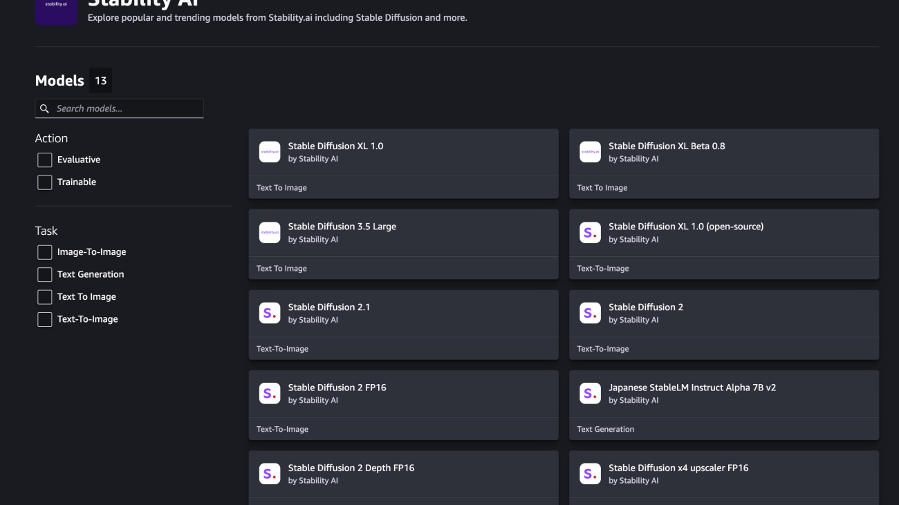


 Tom Yemington is a Senior GenAI Models Specialist focused on helping model providers and customers scale generative AI solutions in AWS. Tom is a Certified Information Systems Security Professional (CISSP). Outside of work, you can find Tom racing vintage cars or teaching people how to race as an instructor at track-day events.
 Isha Dua is a Senior Solutions Architect based in the San Francisco Bay Area working with GENAI Model providers and helping customer optimize their GENAI workloads on AWS. She helps enterprise customers grow by understanding their goals and challenges, and guides them on how they can architect their applications in a cloud-native manner while ensuring resilience and scalability. She’s passionate about machine learning technologies and environmental sustainability.
 Boshi Huang is a Senior Applied Scientist in Generative AI at Amazon Web Services, where he collaborates with customers to develop and implement generative AI solutions. Boshi’s research focuses on advancing the field of generative AI through automatic prompt engineering, adversarial attack and defense mechanisms, inference acceleration, and developing methods for responsible and reliable visual content generation.
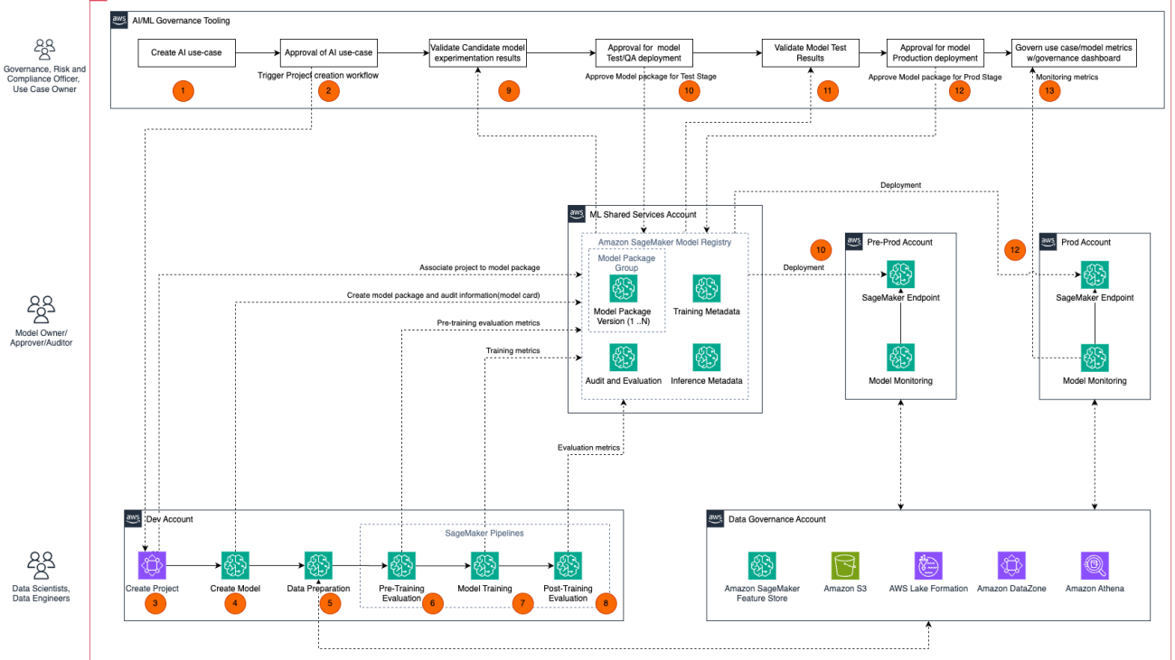


 Ram Vittal is a Principal ML Solutions Architect at AWS. He has over 3 decades of experience architecting and building distributed, hybrid, and cloud applications. He is passionate about building secure and scalable AI/ML and big data solutions to help enterprise customers with their cloud adoption and optimization journey to improve their business outcomes. In his spare time, he rides his motorcycle and walks with his 3-year-old Sheepadoodle.
 Neelam Koshiya is principal solutions architect (GenAI specialist) at AWS. With a background in software engineering, she moved organically into an architecture role. Her current focus is to help enterprise customers with their ML/ GenAI journeys for strategic business outcomes. Her area of depth is machine learning. In her spare time, she enjoys reading and being outdoors.
 Siamak Nariman is a Senior Product Manager at AWS. He is focused on AI/ML technology, ML model management, and ML governance to improve overall organizational efficiency and productivity. He has extensive experience automating processes and deploying various technologies.
 Saumitra Vikaram is a Senior Software Engineer at AWS. He is focused on AI/ML technology, ML model management, ML governance, and MLOps to improve overall organizational efficiency and productivity.
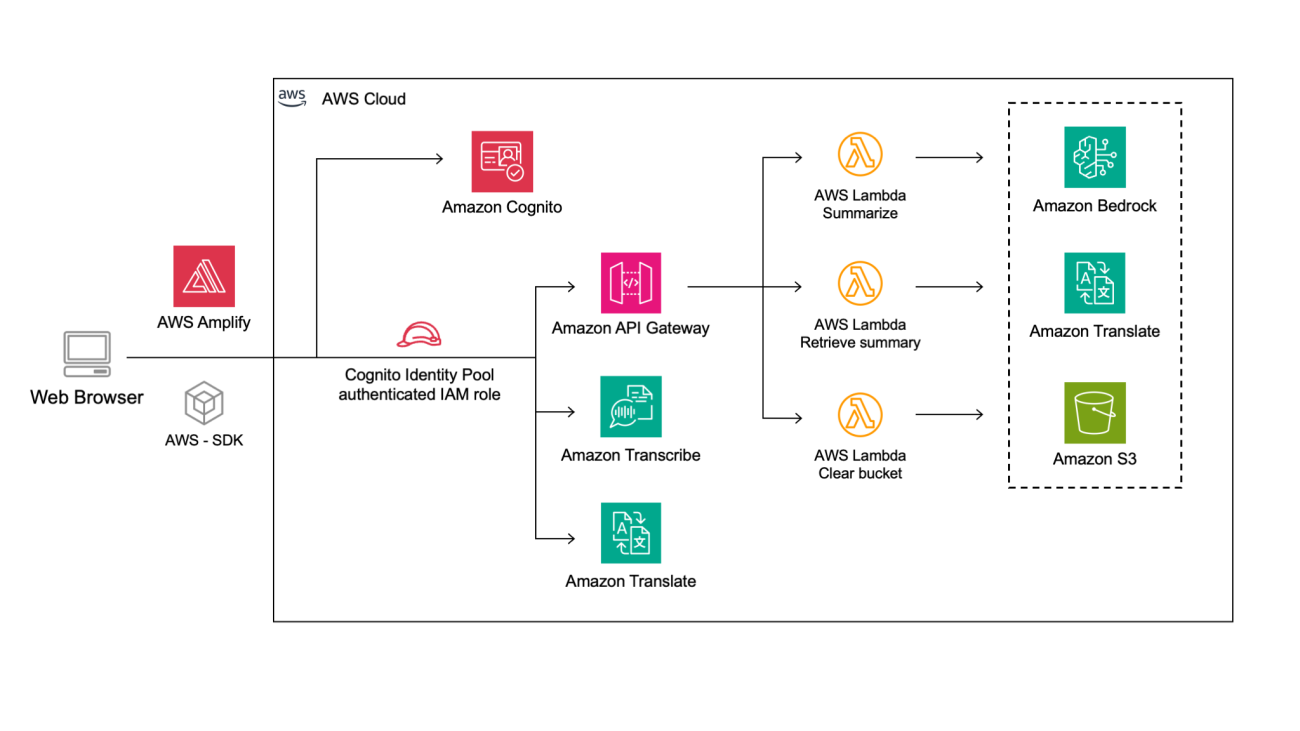


 Luca Guida is a Senior Solutions Architect at AWS; he is based in Milan and he supports independent software vendors in their cloud journey. With an academic background in computer science and engineering, he started developing his AI/ML passion at university; as a member of the natural language processing and generative AI community within AWS, Luca helps customers be successful while adopting AI/ML services.
 Chiara Relandini is an Associate Solutions Architect at AWS. She collaborates with customers from diverse sectors, including digital native businesses and independent software vendors. After focusing on ML during her studies, Chiara supports customers in using generative AI and ML technologies effectively, helping them extract maximum value from these powerful tools.
 Arian Rezai Tabrizi is an Associate Solutions Architect based in Milan. She supports enterprises across various industries, including retail, fashion, and manufacturing, on their cloud journey. Drawing from her background in data science, Arian assists customers in effectively using generative AI and other AI technologies.
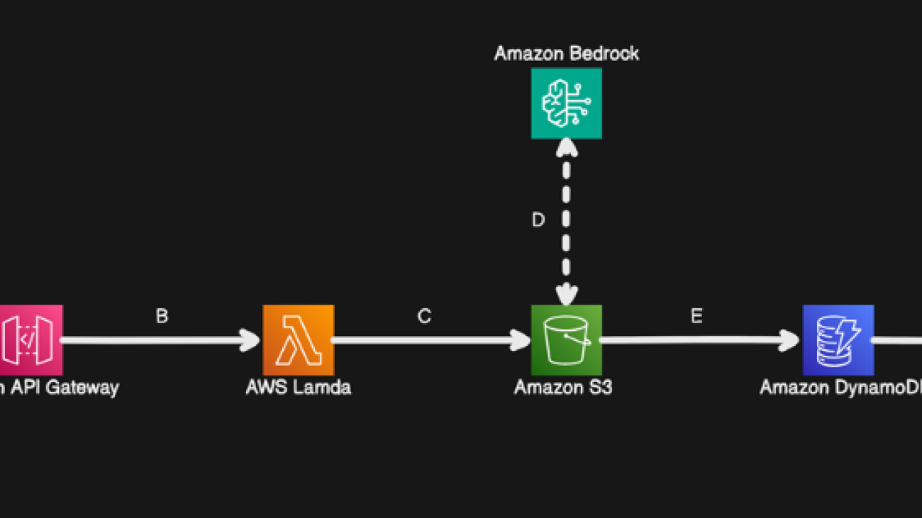


 Jason D’Alba is an AWS Solutions Architect leader focused on enterprise applications, helping customers architect highly available and scalable data & ai solutions.
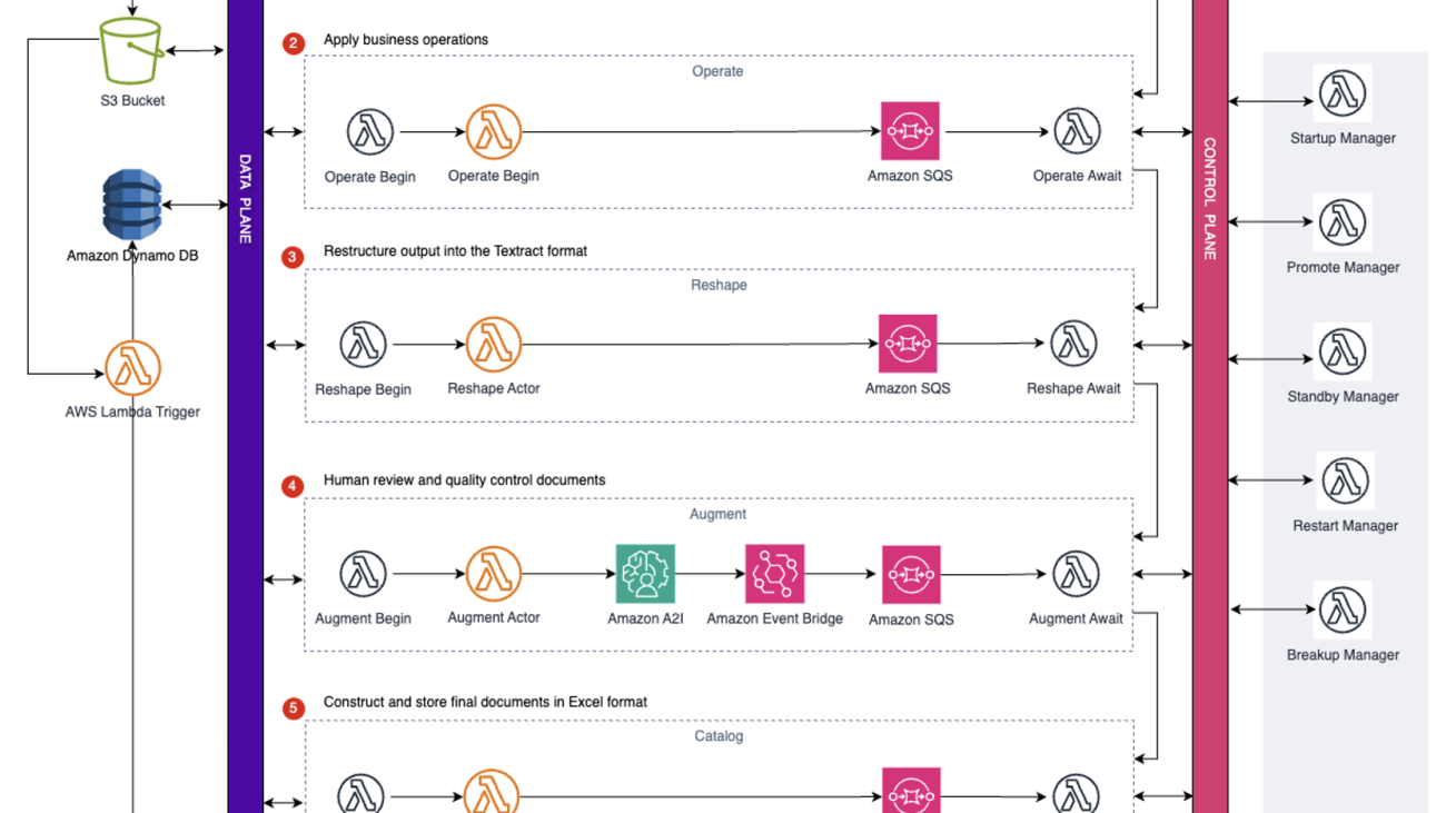


 Marin Mestrovic is a Partner Solutions Architect at Amazon Web Services, specializing in supporting partner solutions. In his role, he collaborates with leading Global System Integrators (GSIs) and independent software vendors (ISVs) to help design and build cost-efficient, scalable, industry-specific solutions. With his expertise in AWS capabilities, Marin empowers partners to develop innovative solutions that drive business growth for their clients.
 Dilin Joy is a Senior Partner Solutions Architect at Amazon Web Services. In his role, he works with leading independent software vendors (ISVs) and Global System Integrators (GSIs) to provide architectural guidance and support in building strategic industry solutions on the AWS platform. His expertise and collaborative approach help these partners develop innovative cloud-based solutions that drive business success for their clients.
 Anjan Biswas is a Senior AI Services Solutions Architect who focuses on computer vision, NLP, and generative AI. Anjan is part of the worldwide AI services specialist team and works with customers to help them understand and develop solutions to business problems with AWS AI Services and generative AI.
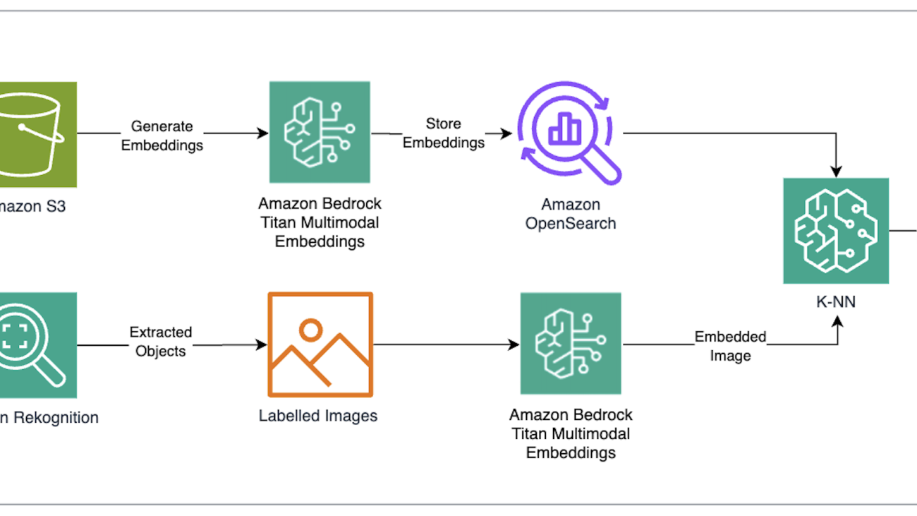
 The steps of the solution include:


 Nathan Pogue is a Solutions Architect on the Canadian Public Sector Healthcare and Life Sciences team at AWS. Based in Toronto, he focuses on empowering his customers to expand their understanding of AWS and utilize the cloud for innovative use cases. He is particularly passionate about AI/ML and enjoys building proof-of-concept solutions for his customers.
 Waleed Malik is a Solutions Architect with the Canadian Public Sector EdTech team at AWS. He holds six AWS certifications, including the Machine Learning Specialty Certification. Waleed is passionate about helping customers deepen their knowledge of AWS by translating their business challenges into technical solutions.
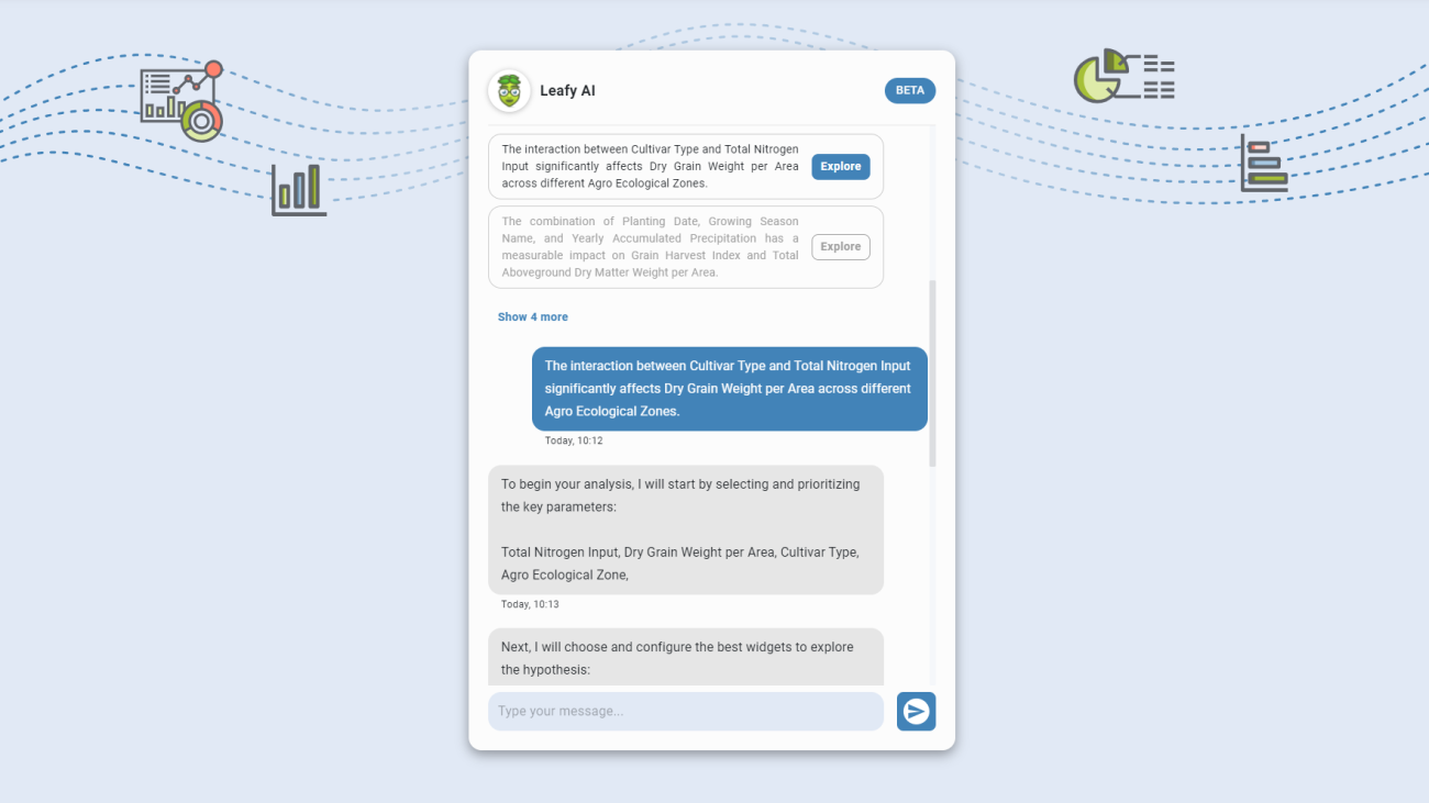

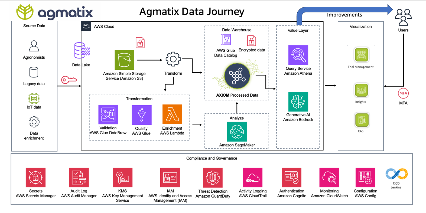
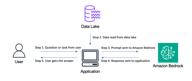

 Etzik Bega is the Chief Architect of Agmatix, where he has revolutionized the company’s data lake architecture using cutting-edge GenAI technology. With over 25 years of experience in cybersecurity, system architecture, and communications, Etzik has recently focused on helping organizations move to the public cloud securely and efficiently.
 Menachem Melamed is a Senior Solutions Architect at AWS, specializing in Big Data analytics and AI. With a deep background in software development and cloud architecture, he empowers organizations to build innovative solutions using modern cloud technologies.
 Prerana Sharma is Manager of Solutions Architects at AWS, specializing in Manufacturing. With a wide experience of working in the Digital Farming space, Prerana helps customers solve business problems by experimenting and innovating with emerging technologies on AWS.
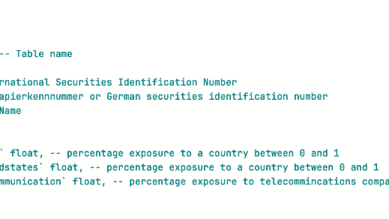


 Randy DeFauw is a Senior Principal Solutions Architect at AWS. He holds an MSEE from the University of Michigan, where he worked on computer vision for autonomous vehicles. He also holds an MBA from Colorado State University. Randy has held a variety of positions in the technology space, ranging from software engineering to product management. In entered the Big Data space in 2013 and continues to explore that area. He is actively working on projects in the ML space and has presented at numerous conferences including Strata and GlueCon.
 Arghya Banerjee is a Sr. Solutions Architect at AWS in the San Francisco Bay Area focused on helping customers adopt and use AWS Cloud. He is focused on Big Data, Data Lakes, Streaming and batch Analytics services and generative AI technologies.
 Ravi Ganesh is a Sr Solution Architect in AWS at Austin Texas Area, focused on helping customer address their business problems through adoption of Cloud, He is focussed on Analytics, Resiliency, Security and Generative AI technologies.
 Varun Mehta is a Sr. Solutions Architect at AWS. He is passionate about helping customers build enterprise-scale Well-Architected solutions on the AWS Cloud. He works with strategic customers who are using AI/ML to solve complex business problems. Outside of work, he loves to spend time with his wife and kids
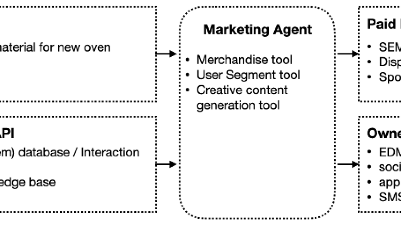


 Ray Wang is a Senior Solutions Architect at AWS. With 10 years of experience in the IT industry, Ray is dedicated to building modern solutions on the cloud, especially in NoSQL, big data, machine learning, and Generative AI. As a hungry go-getter, he passed all 12 AWS certificates to make his technical field not only deep but wide. He loves to read and watch sci-fi movies in his spare time.
 Paul Lu is a Senior Solution Architect at Amazon Web Services (AWS). He specialize in Serverless and modern application development, helping customers design high-performing, scalable cloud solutions. With extensive experience, he is passionate about driving innovation and delivering exceptional results.