 An overview of how we’re expanding code assistance features to all Colab users.Read More

An overview of how we’re expanding code assistance features to all Colab users.Read More

Fifteen minutes. That’s how long it took to empty the Colosseum, an engineering marvel that’s still standing as the largest amphitheater in the world. Two thousand years later, this design continues to work well to move enormous crowds out of sporting and entertainment venues.
But of course, exiting the arena is only the first step. Next, people must navigate the traffic that builds up in the surrounding streets. This is an age-old problem that remains unsolved to this day. In Rome, they addressed the issue by prohibiting private traffic on the street that passes directly by the Colosseum. This policy worked there, but what if you’re not in Rome? What if you’re at the Superbowl? Or at a Taylor Swift concert?
An approach to addressing this problem is to use simulation models, sometimes called “digital twins”, which are virtual replicas of real-world transportation networks that attempt to capture every detail from the layout of streets and intersections to the flow of vehicles. These models allow traffic experts to mitigate congestion, reduce accidents, and improve the experience of drivers, riders, and walkers alike. Previously, our team used these models to quantify sustainability impact of routing, test evacuation plans and show simulated traffic in Maps Immersive View.
Calibrating high-resolution traffic simulations to match the specific dynamics of a particular setting is a longstanding challenge in the field. The availability of aggregate mobility data, detailed Google Maps road network data, advances in transportation science (such as understanding the relationship between segment demands and speeds for road segments with traffic signals), and calibration techniques which make use of speed data in physics-informed traffic models are paving the way for compute-efficient optimization at a global scale.
To test this technology in the real world, Google Research partnered with the Seattle Department of Transportation (SDOT) to develop simulation-based traffic guidance plans. Our goal is to help thousands of attendees of major sports and entertainment events leave the stadium area quickly and safely. The proposed plan reduced average trip travel times by 7 minutes for vehicles leaving the stadium region during large events. We deployed it in collaboration with SDOT using Dynamic Message Signs (DMS) and verified impact over multiple events between August and November, 2023.
 |
 |
| One policy recommendation we made was to divert traffic from S Spokane St, a major thoroughfare that connects the area to highways I-5 and SR 99, and is often congested after events. Suggested changes improved the flow of traffic through highways and arterial streets near the stadium, and reduced the length of vehicle queues that formed behind traffic signals. (Note that vehicles are larger than reality in this clip for demonstration.) |
For this project, we created a new simulation model of the area around Seattle’s stadiums. The intent for this model is to replay each traffic situation for a specified day as closely as possible. We use an open-source simulation software, Simulation of Urban MObility (SUMO). SUMO’s behavioral models help us describe traffic dynamics, for instance, how drivers make decisions, like car-following, lane-changing and speed limit compliance. We also use insights from Google Maps to define the network’s structure and various static segment attributes (e.g., number of lanes, speed limit, presence of traffic lights).
 |
| Overview of the Simulation framework. |
Travel demand is an important simulator input. To compute it, we first decompose the road network of a given metropolitan area into zones, specifically level 13 S2 cells with 1.27 km2 area per cell. From there, we define the travel demand as the expected number of trips that travel from an origin zone to a destination zone in a given time period. The demand is represented as aggregated origin–destination (OD) matrices.
To get the initial expected number of trips between an origin zone and a destination zone, we use aggregated and anonymized mobility statistics. Then we solve the OD calibration problem by combining initial demand with observed traffic statistics, like segment speeds, travel times and vehicular counts, to reproduce event scenarios.
We model the traffic around multiple past events in Seattle’s T-Mobile Park and Lumen Field and evaluate the accuracy by computing aggregated and anonymized traffic statistics. Analyzing these event scenarios helps us understand the effect of different routing policies on congestion in the region.
 |
| Heatmaps demonstrate a substantial increase in numbers of trips in the region after a game as compared to the same time on a non-game day. |
 |
| The graph shows observed segment speeds on the x-axis and simulated speeds on the y-axis for a modeled event. The concentration of data points along the red x=y line demonstrates the ability of the simulation to reproduce realistic traffic conditions. |
SDOT and the Seattle Police Department’s (SPD) local knowledge helped us determine the most congested routes that needed improvement:
We developed routing policies and evaluated them using the simulation model. To disperse traffic faster, we tried policies that would route northbound/southbound traffic from the nearest ramps to further highway ramps, to shorten the wait times. We also experimented with opening HOV lanes to event traffic, recommending alternate routes (e.g., SR 99), or load sharing between different lanes to get to the nearest stadium ramps.


We model multiple events with different traffic conditions, event times, and attendee counts. For each policy, the simulation reproduces post-game traffic and reports the travel time for vehicles, from departing the stadium to reaching their destination or leaving the Seattle SODO area. The time savings are computed as the difference of travel time before/after the policy, and are shown in the below table, per policy, for small and large events. We apply each policy to a percentage of traffic, and re-estimate the travel times. Results are shown if 10%, 30%, or 50% of vehicles are affected by a policy.

Based on these simulation results, the feasibility of implementation, and other considerations, SDOT has decided to implement the “Northbound Cherry St ramp” and “Southbound S Spokane St ramp” policies using DMS during large events. The signs suggest drivers take alternative routes to reach their destinations. The combination of these two policies leads to an average of 7 minutes of travel time savings per vehicle, based on rerouting 30% of traffic during large events.
This work demonstrates the power of simulations to model, identify, and quantify the effect of proposed traffic guidance policies. Simulations allow network planners to identify underused segments and evaluate the effects of different routing policies, leading to a better spatial distribution of traffic. The offline modeling and online testing show that our approach can reduce total travel time. Further improvements can be made by adding more traffic management strategies, such as optimizing traffic lights. Simulation models have been historically time consuming and hence affordable only for the largest cities and high stake projects. By investing in more scalable techniques, we hope to bring these models to more cities and use cases around the world.
In collaboration with Alex Shashko, Andrew Tomkins, Ashley Carrick, Carolina Osorio, Chao Zhang, Damien Pierce, Iveel Tsogsuren, Sheila de Guia, and Yi-fan Chen. Visual design by John Guilyard. We would like to thank our SDOT partners Carter Danne, Chun Kwan, Ethan Bancroft, Jason Cambridge, Laura Wojcicki, Michael Minor, Mohammed Said, Trevor Partap, and SPD partners Lt. Bryan Clenna and Sgt. Brian Kokesh.

With the recent and accelerated advances in machine learning (ML), machines can understand natural language, engage in conversations, draw images, create videos and more. Modern ML models are programmed and trained using ML programming frameworks, such as TensorFlow, JAX, PyTorch, among many others. These libraries provide high-level instructions to ML practitioners, such as linear algebra operations (e.g., matrix multiplication, convolution, etc.) and neural network layers (e.g., 2D convolution layers, transformer layers). Importantly, practitioners need not worry about how to make their models run efficiently on hardware because an ML framework will automatically optimize the user’s model through an underlying compiler. The efficiency of the ML workload, thus, depends on how good the compiler is. A compiler typically relies on heuristics to solve complex optimization problems, often resulting in suboptimal performance.
In this blog post, we present exciting advancements in ML for ML. In particular, we show how we use ML to improve efficiency of ML workloads! Prior works, both internal and external, have shown that we can use ML to improve performance of ML programs by selecting better ML compiler decisions. Although there exist a few datasets for program performance prediction, they target small sub-programs, such as basic blocks or kernels. We introduce “TpuGraphs: A Performance Prediction Dataset on Large Tensor Computational Graphs” (presented at NeurIPS 2023), which we recently released to fuel more research in ML for program optimization. We hosted a Kaggle competition on the dataset, which recently completed with 792 participants on 616 teams from 66 countries. Furthermore, in “Learning Large Graph Property Prediction via Graph Segment Training”, we cover a novel method to scale graph neural network (GNN) training to handle large programs represented as graphs. The technique both enables training arbitrarily large graphs on a device with limited memory capacity and improves generalization of the model.
ML compilers are software routines that convert user-written programs (here, mathematical instructions provided by libraries such as TensorFlow) to executables (instructions to execute on the actual hardware). An ML program can be represented as a computation graph, where a node represents a tensor operation (such as matrix multiplication), and an edge represents a tensor flowing from one node to another. ML compilers have to solve many complex optimization problems, including graph-level and kernel-level optimizations. A graph-level optimization requires the context of the entire graph to make optimal decisions and transforms the entire graph accordingly. A kernel-level optimization transforms one kernel (a fused subgraph) at a time, independently of other kernels.
 |
| Important optimizations in ML compilers include graph-level and kernel-level optimizations. |
To provide a concrete example, imagine a matrix (2D tensor):
 |
It can be stored in computer memory as [A B C a b c] or [A a B b C c], known as row- and column-major memory layout, respectively. One important ML compiler optimization is to assign memory layouts to all intermediate tensors in the program. The figure below shows two different layout configurations for the same program. Let’s assume that on the left-hand side, the assigned layouts (in red) are the most efficient option for each individual operator. However, this layout configuration requires the compiler to insert a copy operation to transform the memory layout between the add and convolution operations. On the other hand, the right-hand side configuration might be less efficient for each individual operator, but it doesn’t require the additional memory transformation. The layout assignment optimization has to trade off between local computation efficiency and layout transformation overhead.
 |
| A node represents a tensor operator, annotated with its output tensor shape [n0, n1, …], where ni is the size of dimension i. Layout {d0, d1, …} represents minor-to-major ordering in memory. Applied configurations are highlighted in red, and other valid configurations are highlighted in blue. A layout configuration specifies the layouts of inputs and outputs of influential operators (i.e., convolution and reshape). A copy operator is inserted when there is a layout mismatch. |
If the compiler makes optimal choices, significant speedups can be made. For example, we have seen up to a 32% speedup when choosing an optimal layout configuration over the default compiler’s configuration in the XLA benchmark suite.
Given the above, we aim to improve ML model efficiency by improving the ML compiler. Specifically, it can be very effective to equip the compiler with a learned cost model that takes in an input program and compiler configuration and then outputs the predicted runtime of the program.
With this motivation, we release TpuGraphs, a dataset for learning cost models for programs running on Google’s custom Tensor Processing Units (TPUs). The dataset targets two XLA compiler configurations: layout (generalization of row- and column-major ordering, from matrices, to higher dimension tensors) and tiling (configurations of tile sizes). We provide download instructions and starter code on the TpuGraphs GitHub. Each example in the dataset contains a computational graph of an ML workload, a compilation configuration, and the execution time of the graph when compiled with the configuration. The graphs in the dataset are collected from open-source ML programs, featuring popular model architectures, e.g., ResNet, EfficientNet, Mask R-CNN, and Transformer. The dataset provides 25× more graphs than the largest (earlier) graph property prediction dataset (with comparable graph sizes), and graph size is 770× larger on average compared to existing performance prediction datasets on ML programs. With this greatly expanded scale, for the first time we can explore the graph-level prediction task on large graphs, which is subject to challenges such as scalability, training efficiency, and model quality.
 |
| Scale of TpuGraphs compared to other graph property prediction datasets. |
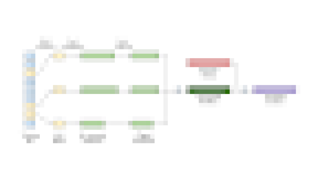
We provide baseline learned cost models with our dataset (architecture shown below). Our baseline models are based on a GNN since the input program is represented as a graph. Node features, shown in blue below, consist of two parts. The first part is an opcode id, the most important information of a node, which indicates the type of tensor operation. Our baseline models, thus, map an opcode id to an opcode embedding via an embedding lookup table. The opcode embedding is then concatenated with the second part, the rest of the node features, as inputs to a GNN. We combine the node embeddings produced by the GNN to create the fixed-size embedding of the graph using a simple graph pooling reduction (i.e., sum and mean). The resulting graph embedding is then linearly transformed into the final scalar output by a feedforward layer.
 |
| Our baseline learned cost model employs a GNN since programs can be naturally represented as graphs. |
Furthermore we present Graph Segment Training (GST), a method for scaling GNN training to handle large graphs on a device with limited memory capacity in cases where the prediction task is on the entire-graph (i.e., graph-level prediction). Unlike scaling training for node- or edge-level prediction, scaling for graph-level prediction is understudied but crucial to our domain, as computation graphs can contain hundreds of thousands of nodes. In a typical GNN training (“Full Graph Training”, on the left below), a GNN model is trained using an entire graph, meaning all nodes and edges of the graph are used to compute gradients. For large graphs, this might be computationally infeasible. In GST, each large graph is partitioned into smaller segments, and a random subset of segments is selected to update the model; embeddings for the remaining segments are produced without saving their intermediate activations (to avoid consuming memory). The embeddings of all segments are then combined to generate an embedding for the original large graph, which is then used for prediction. In addition, we introduce the historical embedding table to efficiently obtain graph segments’ embeddings and segment dropout to mitigate the staleness from historical embeddings. Together, our complete method speeds up the end-to-end training time by 3×.
 |
| Comparing Full Graph Training (typical method) vs Graph Segment Training (our proposed method). |
Finally, we ran the “Fast or Slow? Predict AI Model Runtime” competition over the TpuGraph dataset. This competition ended with 792 participants on 616 teams. We had 10507 submissions from 66 countries. For 153 users (including 47 in the top 100), this was their first competition. We learned many interesting new techniques employed by the participating teams, such as:
We will debrief the competition and preview the winning solutions at the competition session at the ML for Systems workshop at NeurIPS on December 16, 2023. Finally, congratulations to all the winners and thank you for your contributions to advancing research in ML for systems!
If you are interested in more research about structured data and artificial intelligence, we hosted the NeurIPS Expo panel Graph Learning Meets Artificial Intelligence on December 9, which covered advancing learned cost models and more!
Sami Abu-el-Haija (Google Research) contributed significantly to this work and write-up. The research in this post describes joint work with many additional collaborators including Mike Burrows, Kaidi Cao, Bahare Fatemi, Jure Leskovec, Charith Mendis, Dustin Zelle, and Yanqi Zhou.

Text-to-image models trained on large volumes of image-text pairs have enabled the creation of rich and diverse images encompassing many genres and themes. Moreover, popular styles such as “anime” or “steampunk”, when added to the input text prompt, may translate to specific visual outputs. While many efforts have been put into prompt engineering, a wide range of styles are simply hard to describe in text form due to the nuances of color schemes, illumination, and other characteristics. As an example, “watercolor painting” may refer to various styles, and using a text prompt that simply says “watercolor painting style” may either result in one specific style or an unpredictable mix of several.
 |
| When we refer to “watercolor painting style,” which do we mean? Instead of specifying the style in natural language, StyleDrop allows the generation of images that are consistent in style by referring to a style reference image*. |
In this blog we introduce “StyleDrop: Text-to-Image Generation in Any Style”, a tool that allows a significantly higher level of stylized text-to-image synthesis. Instead of seeking text prompts to describe the style, StyleDrop uses one or more style reference images that describe the style for text-to-image generation. By doing so, StyleDrop enables the generation of images in a style consistent with the reference, while effectively circumventing the burden of text prompt engineering. This is done by efficiently fine-tuning the pre-trained text-to-image generation models via adapter tuning on a few style reference images. Moreover, by iteratively fine-tuning the StyleDrop on a set of images it generated, it achieves the style-consistent image generation from text prompts.
StyleDrop is a text-to-image generation model that allows generation of images whose visual styles are consistent with the user-provided style reference images. This is achieved by a couple of iterations of parameter-efficient fine-tuning of pre-trained text-to-image generation models. Specifically, we build StyleDrop on Muse, a text-to-image generative vision transformer.
Muse is a state-of-the-art text-to-image generation model based on the masked generative image transformer (MaskGIT). Unlike diffusion models, such as Imagen or Stable Diffusion, Muse represents an image as a sequence of discrete tokens and models their distribution using a transformer architecture. Compared to diffusion models, Muse is known to be faster while achieving competitive generation quality.
StyleDrop is built by fine-tuning the pre-trained Muse model on a few style reference images and their corresponding text prompts. There have been many works on parameter-efficient fine-tuning of transformers, including prompt tuning and Low-Rank Adaptation (LoRA) of large language models. Among those, we opt for adapter tuning, which is shown to be effective at fine-tuning a large transformer network for language and image generation tasks in a parameter-efficient manner. For example, it introduces less than one million trainable parameters to fine-tune a Muse model of 3B parameters, and it requires only 1000 training steps to converge.
 |
| Parameter-efficient adapter tuning of Muse. |
While StyleDrop is effective at learning styles from a few style reference images, it is still challenging to learn from a single style reference image. This is because the model may not effectively disentangle the content (i.e., what is in the image) and the style (i.e., how it is being presented), leading to reduced text controllability in generation. For example, as shown below in Step 1 and 2, a generated image of a chihuahua from StyleDrop trained from a single style reference image shows a leakage of content (i.e., the house) from the style reference image. Furthermore, a generated image of a temple looks too similar to the house in the reference image (concept collapse).
We address this issue by training a new StyleDrop model on a subset of synthetic images, chosen by the user or by image-text alignment models (e.g., CLIP), whose images are generated by the first round of the StyleDrop model trained on a single image. By training on multiple synthetic image-text aligned images, the model can easily disentangle the style from the content, thus achieving improved image-text alignment.
 |
| Iterative training with feedback*. The first round of StyleDrop may result in reduced text controllability, such as a content leakage or concept collapse, due to the difficulty of content-style disentanglement. Iterative training using synthetic images, generated by the previous rounds of StyleDrop models and chosen by human or image-text alignment models, improves the text adherence of stylized text-to-image generation. |
We show the effectiveness of StyleDrop by running experiments on 24 distinct style reference images. As shown below, the images generated by StyleDrop are highly consistent in style with each other and with the style reference image, while depicting various contexts, such as a baby penguin, banana, piano, etc. Moreover, the model can render alphabet images with a consistent style.
 |
| Stylized text-to-image generation. Style reference images* are on the left inside the yellow box. Text prompts used are: First row: a baby penguin, a banana, a bench. Second row: a butterfly, an F1 race car, a Christmas tree. Third row: a coffee maker, a hat, a moose. Fourth row: a robot, a towel, a wood cabin. |
 |
| Stylized visual character generation. Style reference images* are on the left inside the yellow box. Text prompts used are: (first row) letter ‘A’, letter ‘B’, letter ‘C’, (second row) letter ‘E’, letter ‘F’, letter ‘G’. |
Below we show generated images by sampling from two personalized generation distributions, one for an object and another for the style.
 |
| Images at the top in the blue border are object reference images from the DreamBooth dataset (teapot, vase, dog and cat), and the image on the left at the bottom in the red border is the style reference image*. Images in the purple border (i.e. the four lower right images) are generated from the style image of the specific object. |
For the quantitative evaluation, we synthesize images from a subset of Parti prompts and measure the image-to-image CLIP score for style consistency and image-to-text CLIP score for text consistency. We study non–fine-tuned models of Muse and Imagen. Among fine-tuned models, we make a comparison to DreamBooth on Imagen, state-of-the-art personalized text-to-image method for subjects. We show two versions of StyleDrop, one trained from a single style reference image, and another, “StyleDrop (HF)”, that is trained iteratively using synthetic images with human feedback as described above. As shown below, StyleDrop (HF) shows significantly improved style consistency score over its non–fine-tuned counterpart (0.694 vs. 0.556), as well as DreamBooth on Imagen (0.694 vs. 0.644). We observe an improved text consistency score with StyleDrop (HF) over StyleDrop (0.322 vs. 0.313). In addition, in a human preference study between DreamBooth on Imagen and StyleDrop on Muse, we found that 86% of the human raters preferred StyleDrop on Muse over DreamBooth on Imagen in terms of consistency to the style reference image.
 |
StyleDrop achieves style consistency at text-to-image generation using a few style reference images. Google’s AI Principles guided our development of Style Drop, and we urge the responsible use of the technology. StyleDrop was adapted to create a custom style model in Vertex AI, and we believe it could be a helpful tool for art directors and graphic designers — who might want to brainstorm or prototype visual assets in their own styles, to improve their productivity and boost their creativity — or businesses that want to generate new media assets that reflect a particular brand. As with other generative AI capabilities, we recommend that practitioners ensure they align with copyrights of any media assets they use. More results are found on our project website and YouTube video.
This research was conducted by Kihyuk Sohn, Nataniel Ruiz, Kimin Lee, Daniel Castro Chin, Irina Blok, Huiwen Chang, Jarred Barber, Lu Jiang, Glenn Entis, Yuanzhen Li, Yuan Hao, Irfan Essa, Michael Rubinstein, and Dilip Krishnan. We thank owners of images used in our experiments (links for attribution) for sharing their valuable assets.
*See image sources ↩

 Gemini Pro is now available for developers and enterprises to build AI applications.Read More

 Launching Gemini Pro API and four more AI tools: Imagen 2, MedLM, and Duet AI for Developers and Duet AI in Security Operations.Read More


This week the 37th annual Conference on Neural Information Processing Systems (NeurIPS 2023), the biggest machine learning conference of the year, kicks off in New Orleans, LA. Google is proud to be a Diamond Level sponsor of NeurIPS this year and will have a strong presence with >170 accepted papers, two keynote talks, and additional contributions to the broader research community through organizational support and involvement in >20 workshops and tutorials. Google is also proud to be a Platinum Sponsor for both the Women in Machine Learning and LatinX in AI workshops. We look forward to sharing some of our extensive ML research and expanding our partnership with the broader ML research community.
Attending for NeurIPS 2023 in person? Come visit the Google Research booth to learn more about the exciting work we’re doing to solve some of the field’s most interesting challenges. Visit the @GoogleAI X (Twitter) account to find out about Google booth activities (e.g., demos and Q&A sessions).
You can learn more about our latest cutting edge work being presented at the conference in the list below (Google affiliations highlighted in bold). And see Google DeepMind’s blog to learn more about their participation at NeurIPS 2023.
NeurIPS Board: Corinna Cortes
Advisory Board: John C. Platt
Senior Area Chair: Inderjit S. Dhillon
Creative AI Chair: Isabelle Guyon
Program Chair: Amir Globerson
Datasets and Benchmarks Chair: Remi Denton
What You See is What You Read? Improving Text-Image Alignment Evaluation
Presenter: Yonatan Bitton
Monday, Dec 11 | 12:15PM – 1:45PM
Talk like a Graph: Encoding Graphs for Large Language Models
Presenters: Bahar Fatemi, Jonathan Halcrow, Bryan Perozzi
Monday, Dec 11 | 4:00PM – 4:45PM
VisIT-Bench: A Benchmark for Vision-Language Instruction Following Inspired by Real-World Use
Presenter: Yonatan Bitton
Monday, Dec 11 | 4:00PM – 4:45PM
MLCommons Croissant
Presenters: Omar Benjelloun, Meg Risdal, Lora Aroyo
Tuesday, Dec 12 | 9:15AM – 10:00AM
DaTaSeg: Taming a Universal Multi-Dataset Multi-Task Segmentation Model
Presenter: Xiuye Gu
Tuesday, Dec 12 | 12:45PM – 2:15PM
Embedding Large Graphs
Presenters: Bryan Perozzi, Anton Tsitsulin
Tuesday, Dec 12 | 3:20PM – 3:40PM
Correlated Noise Provably Beats Independent Noise for Differentially Private Learning
Presenter: Krishna Pillutla
Tuesday, Dec 12 | 3:20PM – 3:40PM
Med-PaLM
Presenter: Tao Tu
Tuesday, Dec 12 | 4:45PM – 5:15PM
StyleDrop: Text-to-Image Generation in Any Style
Presenters: Kihyuk Sohn, Lu Jiang, Irfan Essa
Tuesday, Dec 12 | 4:45PM – 5:15PM
DICES Dataset: Diversity in Conversational AI Evaluation for Safety
Presenters: Lora Aroyo, Alicia Parrish, Vinodkumar Prabhakaran
Wednesday, Dec 13 | 9:15AM – 10:00AM
Resonator: Scalable Game-Based Evaluation of Large Models
Presenters: Erin Drake Kajioka, Michal Todorovic
Wednesday, Dec 13 | 12:45PM – 2:15PM
Adversarial Nibbler
Presenter: Lora Aroyo
Wednesday, Dec 13 | 12:45PM – 2:15PM
Towards Generalist Biomedical AI
Presenter: Tao Tu
Wednesday, Dec 13 | 3:15PM – 3:30PM
Conditional Adaptors
Presenter: Junwen Bai
Wednesday, Dec 13 | 3:15PM – 3:30PM
Patient Assistance with Multimodal RAG
Presenters: Ryan Knuffman, Milica Cvetkovic
Wednesday, Dec 13 | 4:15PM – 5:00PM
How Hessian Structure Explains Mysteries in Sharpness Regularization
Presenter: Hossein Mobahi
Wednesday, Dec 13 | 4:15PM – 5:00PM
The Many Faces of Responsible AI
Speaker: Lora Aroyo
Sketching: Core Tools, Learning-Augmentation, and Adaptive Robustness
Speaker: Jelani Nelson
Women in ML
Google Sponsored – Platinum
LatinX in AI
Google Sponsored – Platinum
New in ML
Organizer: Isabelle Guyon
AI for Accelerated Materials Design (AI4Mat-2023)
Fireside Chat: Gowoon Cheon
Associative Memory & Hopfield Networks in 2023
Panelist: Blaise Agüera y Arcas
Information-Theoretic Principles in Cognitive Systems (InfoCog)
Speaker: Alexander Alemi
Machine Learning and the Physical Sciences
Speaker: Alexander Alemi
UniReps: Unifying Representations in Neural Models
Organizer: Mathilde Caron
Robustness of Zero/Few-shot Learning in Foundation Models (R0-FoMo)
Speaker: Partha Talukdar
Organizer: Ananth Balashankar, Yao Qin, Ahmad Beirami
Workshop on Diffusion Models
Speaker: Tali Dekel
Algorithmic Fairness through the Lens of Time
Roundtable Lead: Stephen Pfohl
Organizer: Golnoosh Farnadi
Backdoors in Deep Learning: The Good, the Bad, and the Ugly
Organizer: Eugene Bagdasaryan
OPT 2023: Optimization for Machine Learning
Organizer: Cristóbal Guzmán
Machine Learning for Creativity and Design
Speaker: Aleksander Holynski, Alexander Mordvintsev
Robot Learning Workshop: Pretraining, Fine-Tuning, and Generalization with Large Scale Models
Speaker: Matt Barnes
Machine Learning for Audio
Organizer: Shrikanth Narayanan
Federated Learning in the Age of Foundation Models (FL@FM-NeurIPS’23)
Speaker: Cho-Jui Hsieh, Zheng Xu
Socially Responsible Language Modelling Research (SoLaR)
Panelist: Vinodkumar Prabhakaran
I Can’t Believe It’s Not Better (ICBINB): Failure Modes in the Age of Foundation Models
Advisory Board: Javier Antorán
Machine Learning for Systems
Organizer: Yawen Wang
Competition Committee: Bryan Perozzi, Sami Abu-el-haija
Steering Committee: Milad Hashemi
Self-Supervised Learning: Theory and Practice
Organizer: Mathilde Caron
NeurIPS 2023 Machine Unlearning Competition
Organizer: Isabelle Guyon, Peter Kairouz
Lux AI Challenge Season 2 NeurIPS Edition
Organizer: Bovard Doerschuk-Tiberi, Addison Howard
Data-Centric AI for Reliable and Responsible AI: From Theory to Practice
Isabelle Guyon, Nabeel Seedat, Mihaela va der Schaar
Creative AI Performances 1 & 2
Speaker: Erin Drake Kajioka, Yonatan Bitton
Organizer: Isabelle Guyon
Performance 1: Mon, Dec 11 | 6:30PM – 8:30PM, Lobby Stage
Performance 2: Thu, Dec 14 | 7:00PM – 9:00PM, Lobby Stage
Creative AI Sessions 1 – 3
Speaker: Erin Drake Kajioka, Yonatan Bitton
Organizer: Isabelle Guyon
Session 1: Tue, Dec 12 | 3:05PM – 3:40PM, Hall D2
Session 2: Wed, Dec 13 | 10:45AM – 2:15PM, Hall D2
Session 3: Thu, Dec 14 | 10:45 AM – 2:15PM, Hall D2
Creative AI Videos
Organizer: Isabelle Guyon
Graph Learning Meets Artificial Intelligence
Speaker: Bryan Perozzi
Resonator: Music Space
Speakers: Erin Drake Kajioka, Michal Todorovic
Empirical Rigor in ML as a Massively Parallelizable Challenge
Speaker: Megan Risdal (Kaggle)
Ordering-based Conditions for Global Convergence of Policy Gradient Methods
Jincheng Mei, Bo Dai, Alekh Agarwal, Mohammad Ghavamzadeh*, Csaba Szepesvari, Dale Schuurmans
Private Everlasting Prediction
Moni Naor, Kobbi Nissim, Uri Stemmer, Chao Yan
User-Level Differential Privacy With Few Examples Per User
Badih Ghazi, Pritish Kamath, Ravi Kumar, Pasin Manurangsi, Raghu Meka, Chiyuan Zhang
DataComp: In Search of the Next Generation of Multimodal Datasets
Samir Yitzhak Gadre, Gabriel Ilharco, Alex Fang, Jonathan Hayase, Georgios Smyrnis, Thao Nguyen, Ryan Marten, Mitchell Wortsman, Dhruba Ghosh, Jieyu Zhang, Eyal Orgad, Rahim Entezari, Giannis Daras, Sarah Pratt, Vivek Ramanujan, Yonatan Bitton, Kalyani Marathe, Stephen Mussmann, Richard Vencu, Mehdi Cherti, Ranjay Krishna, Pang Wei Koh, Olga Saukh, Alexander Ratner, Shuran Song, Hannaneh Hajishirzi, Ali Farhadi, Romain Beaumont, Sewoong Oh, Alex Dimakis, Jenia Jitsev, Yair Carmon, Vaishaal Shankar, Ludwig Schmidt
Optimal Learners for Realizable Regression: PAC Learning and Online Learning
Idan Attias, Steve Hanneke, Alkis Kalavasis, Amin Karbasi, Grigoris Velegkas
The Surprising Effectiveness of Diffusion Models for Optical Flow and Monocular Depth Estimation
Saurabh Saxena, Charles Herrmann, Junhwa Hur, Abhishek Kar, Mohammad Norouzi*, Deqing Sun, David J. Fleet
Graph Clustering with Graph Neural Networks
Anton Tsitsulin, John Palowitch, Bryan Perozzi, Emmanuel Müller
Alternating Updates for Efficient Transformers (see blog post)
Cenk Baykal, Dylan Cutler, Nishanth Dikkala, Nikhil Ghosh*, Rina Panigrahy, Xin Wang
Does Localization Inform Editing? Surprising Differences in Causality-Based Localization vs. Knowledge Editing in Language Models
Peter Hase, Mohit Bansal, Been Kim, Asma Ghandeharioun
Is Learning in Games Good for the Learners?
William Brown, Jon Schneider, Kiran Vodrahalli
Participatory Personalization in Classification
Hailey Joren, Chirag Nagpal, Katherine Heller, Berk Ustun
Tight Risk Bounds for Gradient Descent on Separable Data
Matan Schliserman, Tomer Koren
Counterfactual Memorization in Neural Language Models
Chiyuan Zhang, Daphne Ippolito, Katherine Lee, Matthew Jagielski, Florian Tramèr, Nicholas Carlini
Debias Coarsely, Sample Conditionally: Statistical Downscaling through Optimal Transport and Probabilistic Diffusion Models
Zhong Yi Wan, Ricardo Baptista, Anudhyan Boral, Yi-Fan Chen, John Anderson, Fei Sha, Leonardo Zepeda-Nunez
Faster Margin Maximization Rates for Generic Optimization Methods
Guanghui Wang, Zihao Hu, Vidya Muthukumar, Jacob Abernethy
From Pixels to UI Actions: Learning to Follow Instructions via Graphical User Interfaces
Peter Shaw, Mandar Joshi, James Cohan, Jonathan Berant, Panupong Pasupat, Hexiang Hu, Urvashi Khandelwal, Kenton Lee, Kristina N Toutanova
PAC Learning Linear Thresholds from Label Proportions
Anand Brahmbhatt, Rishi Saket, Aravindan Raghuveer
SPAE: Semantic Pyramid AutoEncoder for Multimodal Generation with Frozen LLMs
Lijun Yu*, Yong Cheng, Zhiruo Wang, Vivek Kumar, Wolfgang Macherey, Yanping Huang, David Ross, Irfan Essa, Yonatan Bisk, Ming-Hsuan Yang, Kevin Murphy, Alexander Hauptmann, Lu Jiang
Adaptive Data Analysis in a Balanced Adversarial Model
Kobbi Nissim, Uri Stemmer, Eliad Tsfadia
Lexinvariant Language Models
Qian Huang, Eric Zelikman, Sarah Chen, Yuhuai Wu, Gregory Valiant, Percy Liang
On Quantum Backpropagation, Information Reuse, and Cheating Measurement Collapse
Amira Abbas, Robbie King, Hsin-Yuan Huang, William J. Huggins, Ramis Movassagh, Dar Gilboa, Jarrod McClean
Private Estimation Algorithms for Stochastic Block Models and Mixture Models
Hongjie Chen, Vincent Cohen-Addad, Tommaso d’Orsi, Alessandro Epasto, Jacob Imola, David Steurer, Stefan Tiegel
Provably Fast Finite Particle Variants of SVGD via Virtual Particle Stochastic Approximation
Aniket Das, Dheeraj Nagaraj
Private (Stochastic) Non-Convex Optimization Revisited: Second-Order Stationary Points and Excess Risks
Arun Ganesh, Daogao Liu*, Sewoong Oh, Abhradeep Guha Thakurta
Uncovering the Hidden Dynamics of Video Self-supervised Learning under Distribution Shifts
Pritam Sarkar, Ahmad Beirami, Ali Etemad
AIMS: All-Inclusive Multi-Level Segmentation for Anything
Lu Qi, Jason Kuen, Weidong Guo, Jiuxiang Gu, Zhe Lin, Bo Du, Yu Xu, Ming-Hsuan Yang
DreamHuman: Animatable 3D Avatars from Text
Nikos Kolotouros, Thiemo Alldieck, Andrei Zanfir, Eduard Gabriel Bazavan, Mihai Fieraru, Cristian Sminchisescu
Follow-ups Also Matter: Improving Contextual Bandits via Post-serving Contexts
Chaoqi Wang, Ziyu Ye, Zhe Feng, Ashwinkumar Badanidiyuru, Haifeng Xu
Learning List-Level Domain-Invariant Representations for Ranking
Ruicheng Xian*, Honglei Zhuang, Zhen Qin, Hamed Zamani*, Jing Lu, Ji Ma, Kai Hui, Han Zhao, Xuanhui Wang, Michael Bendersky
Optimal Guarantees for Algorithmic Reproducibility and Gradient Complexity in Convex Optimization
Liang Zhang, Junchi Yang, Amin Karbasi, Niao He
Unified Embedding: Battle-Tested Feature Representations for Web-Scale ML Systems
Benjamin Coleman, Wang-Cheng Kang, Matthew Fahrbach, Ruoxi Wang, Lichan Hong, Ed Chi, Derek Cheng
Proximity-Informed Calibration for Deep Neural Networks
Miao Xiong, Ailin Deng, Pang Wei Koh, Jiaying Wu, Shen Li, Jianqing Xu, Bryan Hooi
Anonymous Learning via Look-Alike Clustering: A Precise Analysis of Model Generalization
Adel Javanmard, Vahab Mirrokni
Better Private Linear Regression Through Better Private Feature Selection
Travis Dick, Jennifer Gillenwater*, Matthew Joseph
Binarized Neural Machine Translation
Yichi Zhang, Ankush Garg, Yuan Cao, Łukasz Lew, Behrooz Ghorbani*, Zhiru Zhang, Orhan Firat
BoardgameQA: A Dataset for Natural Language Reasoning with Contradictory Information
Mehran Kazemi, Quan Yuan, Deepti Bhatia, Najoung Kim, Xin Xu, Vaiva Imbrasaite, Deepak Ramachandran
Boosting with Tempered Exponential Measures
Richard Nock, Ehsan Amid, Manfred Warmuth
Concept Algebra for (Score-Based) Text-Controlled Generative Models
Zihao Wang, Lin Gui, Jeffrey Negrea, Victor Veitch
Deep Contract Design via Discontinuous Networks
Tonghan Wang, Paul Dütting, Dmitry Ivanov, Inbal Talgam-Cohen, David C. Parkes
Diffusion-SS3D: Diffusion Model for Semi-supervised 3D Object Detection
Cheng-Ju Ho, Chen-Hsuan Tai, Yen-Yu Lin, Ming-Hsuan Yang, Yi-Hsuan Tsai
Eliciting User Preferences for Personalized Multi-Objective Decision Making through Comparative Feedback
Han Shao, Lee Cohen, Avrim Blum, Yishay Mansour, Aadirupa Saha, Matthew Walter
Gradient Descent with Linearly Correlated Noise: Theory and Applications to Differential Privacy
Anastasia Koloskova*, Ryan McKenna, Zachary Charles, J Keith Rush, Hugh Brendan McMahan
Hardness of Low Rank Approximation of Entrywise Transformed Matrix Products
Tamas Sarlos, Xingyou Song, David P. Woodruff, Qiuyi (Richard) Zhang
Module-wise Adaptive Distillation for Multimodality Foundation Models
Chen Liang, Jiahui Yu, Ming-Hsuan Yang, Matthew Brown, Yin Cui, Tuo Zhao, Boqing Gong, Tianyi Zhou
Multi-Swap k-Means++
Lorenzo Beretta, Vincent Cohen-Addad, Silvio Lattanzi, Nikos Parotsidis
OpenMask3D: Open-Vocabulary 3D Instance Segmentation
Ayça Takmaz, Elisabetta Fedele, Robert Sumner, Marc Pollefeys, Federico Tombari, Francis Engelmann
Order Matters in the Presence of Dataset Imbalance for Multilingual Learning
Dami Choi*, Derrick Xin, Hamid Dadkhahi, Justin Gilmer, Ankush Garg, Orhan Firat, Chih-Kuan Yeh, Andrew M. Dai, Behrooz Ghorbani
PopSign ASL v1.0: An Isolated American Sign Language Dataset Collected via Smartphones
Thad Starner, Sean Forbes, Matthew So, David Martin, Rohit Sridhar, Gururaj Deshpande, Sam Sepah, Sahir Shahryar, Khushi Bhardwaj, Tyler Kwok, Daksh Sehgal, Saad Hassan, Bill Neubauer, Sofia Vempala, Alec Tan, Jocelyn Heath, Unnathi Kumar, Priyanka Mosur, Tavenner Hall, Rajandeep Singh, Christopher Cui, Glenn Cameron, Sohier Dane, Garrett Tanzer
Semi-Implicit Denoising Diffusion Models (SIDDMs)
Yanwu Xu*, Mingming Gong, Shaoan Xie, Wei Wei, Matthias Grundmann, Kayhan Batmanghelich, Tingbo Hou
State2Explanation: Concept-Based Explanations to Benefit Agent Learning and User Understanding
Devleena Das, Sonia Chernova, Been Kim
StoryBench: A Multifaceted Benchmark for Continuous Story Visualization
Emanuele Bugliarello*, Hernan Moraldo, Ruben Villegas, Mohammad Babaeizadeh, Mohammad Taghi Saffar, Han Zhang, Dumitru Erhan, Vittorio Ferrari, Pieter-Jan Kindermans, Paul Voigtlaender
Subject-driven Text-to-Image Generation via Apprenticeship Learning
Wenhu Chen, Hexiang Hu, Yandong Li, Nataniel Ruiz, Xuhui Jia, Ming-Wei Chang, William W. Cohen
TpuGraphs: A Performance Prediction Dataset on Large Tensor Computational Graphs
Phitchaya Mangpo Phothilimthana, Sami Abu-El-Haija, Kaidi Cao*, Bahare Fatemi, Mike Burrows, Charith Mendis*, Bryan Perozzi
Training Chain-of-Thought via Latent-Variable Inference
Du Phan, Matthew D. Hoffman, David Dohan*, Sholto Douglas, Tuan Anh Le, Aaron Parisi, Pavel Sountsov, Charles Sutton, Sharad Vikram, Rif A. Saurous
Unified Lower Bounds for Interactive High-dimensional Estimation under Information Constraints
Jayadev Acharya, Clement L. Canonne, Ziteng Sun, Himanshu Tyagi
What You See is What You Read? Improving Text-Image Alignment Evaluation
Michal Yarom, Yonatan Bitton, Soravit Changpinyo, Roee Aharoni, Jonathan Herzig, Oran Lang, Eran Ofek, Idan Szpektor
When Does Confidence-Based Cascade Deferral Suffice?
Wittawat Jitkrittum, Neha Gupta, Aditya Krishna Menon, Harikrishna Narasimhan, Ankit Singh Rawat, Sanjiv Kumar
Accelerating Molecular Graph Neural Networks via Knowledge Distillation
Filip Ekström Kelvinius, Dimitar Georgiev, Artur Petrov Toshev, Johannes Gasteiger
AVIS: Autonomous Visual Information Seeking with Large Language Model Agent
Ziniu Hu*, Ahmet Iscen, Chen Sun, Kai-Wei Chang, Yizhou Sun, David Ross, Cordelia Schmid, Alireza Fathi
Beyond Invariance: Test-Time Label-Shift Adaptation for Addressing “Spurious” Correlations
Qingyao Sun, Kevin Patrick Murphy, Sayna Ebrahimi, Alexander D’Amour
Collaborative Score Distillation for Consistent Visual Editing
Subin Kim, Kyungmin Lee, June Suk Choi, Jongheon Jeong, Kihyuk Sohn, Jinwoo Shin
CommonScenes: Generating Commonsense 3D Indoor Scenes with Scene Graphs
Guangyao Zhai, Evin Pınar Örnek, Shun-Cheng Wu, Yan Di, Federico Tombari, Nassir Navab, Benjamin Busam
Computational Complexity of Learning Neural Networks: Smoothness and Degeneracy
Amit Daniely, Nathan Srebro, Gal Vardi
A Computationally Efficient Sparsified Online Newton Method
Fnu Devvrit*, Sai Surya Duvvuri, Rohan Anil, Vineet Gupta, Cho-Jui Hsieh, Inderjit S Dhillon
DDF-HO: Hand-Held Object Reconstruction via Conditional Directed Distance Field
Chenyangguang Zhang, Yan Di, Ruida Zhang, Guangyao Zhai, Fabian Manhardt, Federico Tombari, Xiangyang Ji
Double Auctions with Two-sided Bandit Feedback
Soumya Basu, Abishek Sankararaman
Grammar Prompting for Domain-Specific Language Generation with Large Language Models
Bailin Wang, Zi Wang, Xuezhi Wang, Yuan Cao, Rif A. Saurous, Yoon Kim
Inconsistency, Instability, and Generalization Gap of Deep Neural Network Training
Rie Johnson, Tong Zhang*
Large Graph Property Prediction via Graph Segment Training
Kaidi Cao*, Phitchaya Mangpo Phothilimthana, Sami Abu-El-Haija, Dustin Zelle, Yanqi Zhou, Charith Mendis*, Jure Leskovec, Bryan Perozzi
On Computing Pairwise Statistics with Local Differential Privacy
Badih Ghazi, Pritish Kamath, Ravi Kumar, Pasin Manurangsi, Adam Sealfon
On Student-teacher Deviations in Distillation: Does it Pay to Disobey?
Vaishnavh Nagarajan, Aditya Krishna Menon, Srinadh Bhojanapalli, Hossein Mobahi, Sanjiv Kumar
Optimal Cross-learning for Contextual Bandits with Unknown Context Distributions
Jon Schneider, Julian Zimmert
Near-Optimal k-Clustering in the Sliding Window Model
David Woodruff, Peilin Zhong, Samson Zhou
Post Hoc Explanations of Language Models Can Improve Language Models
Satyapriya Krishna, Jiaqi Ma, Dylan Z Slack, Asma Ghandeharioun, Sameer Singh, Himabindu Lakkaraju
Recommender Systems with Generative Retrieval
Shashank Rajput*, Nikhil Mehta, Anima Singh, Raghunandan Hulikal Keshavan, Trung Vu, Lukasz Heldt, Lichan Hong, Yi Tay, Vinh Q. Tran, Jonah Samost, Maciej Kula, Ed H. Chi, Maheswaran Sathiamoorthy
Reinforcement Learning for Fine-tuning Text-to-Image Diffusion Models
Ying Fan, Olivia Watkins, Yuqing Du, Hao Liu, Moonkyung Ryu, Craig Boutilier, Pieter Abbeel, Mohammad Ghavamzadeh*, Kangwook Lee, Kimin Lee*
Replicable Clustering
Hossein Esfandiari, Amin Karbasi, Vahab Mirrokni, Grigoris Velegkas, Felix Zhou
Replicability in Reinforcement Learning
Amin Karbasi, Grigoris Velegkas, Lin Yang, Felix Zhou
Riemannian Projection-free Online Learning
Zihao Hu, Guanghui Wang, Jacob Abernethy
Sharpness-Aware Minimization Leads to Low-Rank Features
Maksym Andriushchenko, Dara Bahri, Hossein Mobahi, Nicolas Flammarion
What is the Inductive Bias of Flatness Regularization? A Study of Deep Matrix Factorization Models
Khashayar Gatmiry, Zhiyuan Li, Ching-Yao Chuang, Sashank Reddi, Tengyu Ma, Stefanie Jegelka
Block Low-Rank Preconditioner with Shared Basis for Stochastic Optimization
Jui-Nan Yen, Sai Surya Duvvuri, Inderjit S Dhillon, Cho-Jui Hsieh
Blocked Collaborative Bandits: Online Collaborative Filtering with Per-Item Budget Constraints
Soumyabrata Pal, Arun Sai Suggala, Karthikeyan Shanmugam, Prateek Jain
Boundary Guided Learning-Free Semantic Control with Diffusion Models
Ye Zhu, Yu Wu, Zhiwei Deng, Olga Russakovsky, Yan Yan
Conditional Adapters: Parameter-efficient Transfer Learning with Fast Inference
Tao Lei, Junwen Bai, Siddhartha Brahma, Joshua Ainslie, Kenton Lee, Yanqi Zhou, Nan Du*, Vincent Y. Zhao, Yuexin Wu, Bo Li, Yu Zhang, Ming-Wei Chang
Conformal Prediction for Time Series with Modern Hopfield Networks
Andreas Auer, Martin Gauch, Daniel Klotz, Sepp Hochreiter
Does Visual Pretraining Help End-to-End Reasoning?
Chen Sun, Calvin Luo, Xingyi Zhou, Anurag Arnab, Cordelia Schmid
Effective Robustness Against Natural Distribution Shifts for Models with Different Training Data
Zhouxing Shi*, Nicholas Carlini, Ananth Balashankar, Ludwig Schmidt, Cho-Jui Hsieh, Alex Beutel*, Yao Qin
Improving Neural Network Representations Using Human Similarity Judgments
Lukas Muttenthaler*, Lorenz Linhardt, Jonas Dippel, Robert A. Vandermeulen, Katherine Hermann, Andrew K. Lampinen, Simon Kornblith
Label Robust and Differentially Private Linear Regression: Computational and Statistical Efficiency
Xiyang Liu, Prateek Jain, Weihao Kong, Sewoong Oh, Arun Sai Suggala
Mnemosyne: Learning to Train Transformers with Transformers
Deepali Jain, Krzysztof Choromanski, Avinava Dubey, Sumeet Singh, Vikas Sindhwani, Tingnan Zhang, Jie Tan
Nash Regret Guarantees for Linear Bandits
Ayush Sawarni, Soumyabrata Pal, Siddharth Barman
A Near-Linear Time Algorithm for the Chamfer Distance
Ainesh Bakshi, Piotr Indyk, Rajesh Jayaram, Sandeep Silwal, Erik Waingarten.
On Differentially Private Sampling from Gaussian and Product Distributions
Badih Ghazi, Xiao Hu*, Ravi Kumar, Pasin Manurangsi
On Dynamic Programming Decompositions of Static Risk Measures in Markov Decision Processes
Jia Lin Hau, Erick Delage, Mohammad Ghavamzadeh*, Marek Petrik
ResMem: Learn What You Can and Memorize the Rest
Zitong Yang, Michal Lukasik, Vaishnavh Nagarajan, Zonglin Li, Ankit Singh Rawat, Manzil Zaheer, Aditya Krishna Menon, Sanjiv Kumar
Responsible AI (RAI) Games and Ensembles
Yash Gupta, Runtian Zhai, Arun Suggala, Pradeep Ravikumar
RoboCLIP: One Demonstration Is Enough to Learn Robot Policies
Sumedh A Sontakke, Jesse Zhang, Sébastien M. R. Arnold, Karl Pertsch, Erdem Biyik, Dorsa Sadigh, Chelsea Finn, Laurent Itti
Robust Concept Erasure via Kernelized Rate-Distortion Maximization
Somnath Basu Roy Chowdhury, Nicholas Monath, Kumar Avinava Dubey, Amr Ahmed, Snigdha Chaturvedi
Robust Multi-Agent Reinforcement Learning via Adversarial Regularization: Theoretical Foundation and Stable Algorithms
Alexander Bukharin, Yan Li, Yue Yu, Qingru Zhang, Zhehui Chen, Simiao Zuo, Chao Zhang, Songan Zhang, Tuo Zhao
Simplicity Bias in 1-Hidden Layer Neural Networks
Depen Morwani*, Jatin Batra, Prateek Jain, Praneeth Netrapalli
SLaM: Student-Label Mixing for Distillation with Unlabeled Examples
Vasilis Kontonis, Fotis Iliopoulos, Khoa Trinh, Cenk Baykal, Gaurav Menghani, Erik Vee
SNAP: Self-Supervised Neural Maps for Visual Positioning and Semantic Understanding
Paul-Edouard Sarlin*, Eduard Trulls, Marc Pollefeys, Jan Hosang, Simon Lynen
SOAR: Improved Indexing for Approximate Nearest Neighbor Search
Philip Sun, David Simcha, Dave Dopson, Ruiqi Guo, Sanjiv Kumar
StyleDrop: Text-to-Image Synthesis of Any Style
Kihyuk Sohn, Lu Jiang, Jarred Barber, Kimin Lee*, Nataniel Ruiz, Dilip Krishnan, Huiwen Chang*, Yuanzhen Li, Irfan Essa, Michael Rubinstein, Yuan Hao, Glenn Entis, Irina Blok, Daniel Castro Chin
Three Towers: Flexible Contrastive Learning with Pretrained Image Models
Jannik Kossen*, Mark Collier, Basil Mustafa, Xiao Wang, Xiaohua Zhai, Lucas Beyer, Andreas Steiner, Jesse Berent, Rodolphe Jenatton, Efi Kokiopoulou
Two-Stage Learning to Defer with Multiple Experts
Anqi Mao, Christopher Mohri, Mehryar Mohri, Yutao Zhong
AdANNS: A Framework for Adaptive Semantic Search
Aniket Rege, Aditya Kusupati, Sharan Ranjit S, Alan Fan, Qingqing Cao, Sham Kakade, Prateek Jain, Ali Farhadi
Cappy: Outperforming and Boosting Large Multi-Task LMs with a Small Scorer
Bowen Tan*, Yun Zhu, Lijuan Liu, Eric Xing, Zhiting Hu, Jindong Chen
Causal-structure Driven Augmentations for Text OOD Generalization
Amir Feder, Yoav Wald, Claudia Shi, Suchi Saria, David Blei
Dense-Exponential Random Features: Sharp Positive Estimators of the Gaussian Kernel
Valerii Likhosherstov, Krzysztof Choromanski, Avinava Dubey, Frederick Liu, Tamas Sarlos, Adrian Weller
Diffusion Hyperfeatures: Searching Through Time and Space for Semantic Correspondence
Grace Luo, Lisa Dunlap, Dong Huk Park, Aleksander Holynski, Trevor Darrell
Diffusion Self-Guidance for Controllable Image Generation
Dave Epstein, Allan Jabri, Ben Poole, Alexei A Efros, Aleksander Holynski
Fully Dynamic k-Clustering in Õ(k) Update Time
Sayan Bhattacharya, Martin Nicolas Costa, Silvio Lattanzi, Nikos Parotsidis
Improving CLIP Training with Language Rewrites
Lijie Fan, Dilip Krishnan, Phillip Isola, Dina Katabi, Yonglong Tian
<!–k-Means Clustering with Distance-Based Privacy
Alessandro Epasto, Vahab Mirrokni, Shyam Narayanan, Peilin Zhong
–>
LayoutGPT: Compositional Visual Planning and Generation with Large Language Models
Weixi Feng, Wanrong Zhu, Tsu-Jui Fu, Varun Jampani, Arjun Reddy Akula, Xuehai He, Sugato Basu, Xin Eric Wang, William Yang Wang
Offline Reinforcement Learning for Mixture-of-Expert Dialogue Management
Dhawal Gupta*, Yinlam Chow, Azamat Tulepbergenov, Mohammad Ghavamzadeh*, Craig Boutilier
Optimal Unbiased Randomizers for Regression with Label Differential Privacy
Ashwinkumar Badanidiyuru, Badih Ghazi, Pritish Kamath, Ravi Kumar, Ethan Jacob Leeman, Pasin Manurangsi, Avinash V Varadarajan, Chiyuan Zhang
Paraphrasing Evades Detectors of AI-generated Text, but Retrieval Is an Effective Defense
Kalpesh Krishna, Yixiao Song, Marzena Karpinska, John Wieting, Mohit Iyyer
ReMaX: Relaxing for Better Training on Efficient Panoptic Segmentation
Shuyang Sun*, Weijun Wang, Qihang Yu*, Andrew Howard, Philip Torr, Liang-Chieh Chen*
Robust and Actively Secure Serverless Collaborative Learning
Nicholas Franzese, Adam Dziedzic, Christopher A. Choquette-Choo, Mark R. Thomas, Muhammad Ahmad Kaleem, Stephan Rabanser, Congyu Fang, Somesh Jha, Nicolas Papernot, Xiao Wang
SpecTr: Fast Speculative Decoding via Optimal Transport
Ziteng Sun, Ananda Theertha Suresh, Jae Hun Ro, Ahmad Beirami, Himanshu Jain, Felix Yu
Structured Prediction with Stronger Consistency Guarantees
Anqi Mao, Mehryar Mohri, Yutao Zhong
Affinity-Aware Graph Networks
Ameya Velingker, Ali Kemal Sinop, Ira Ktena, Petar Veličković, Sreenivas Gollapudi
ARTIC3D: Learning Robust Articulated 3D Shapes from Noisy Web Image Collections
Chun-Han Yao*, Amit Raj, Wei-Chih Hung, Yuanzhen Li, Michael Rubinstein, Ming-Hsuan Yang, Varun Jampani
Black-Box Differential Privacy for Interactive ML
Haim Kaplan, Yishay Mansour, Shay Moran, Kobbi Nissim, Uri Stemmer
Bypassing the Simulator: Near-Optimal Adversarial Linear Contextual Bandits
Haolin Liu, Chen-Yu Wei, Julian Zimmert
DaTaSeg: Taming a Universal Multi-Dataset Multi-Task Segmentation Model
Xiuye Gu, Yin Cui*, Jonathan Huang, Abdullah Rashwan, Xuan Yang, Xingyi Zhou, Golnaz Ghiasi, Weicheng Kuo, Huizhong Chen, Liang-Chieh Chen*, David Ross
Easy Learning from Label Proportions
Robert Busa-Fekete, Heejin Choi*, Travis Dick, Claudio Gentile, Andres Munoz Medina
Efficient Data Subset Selection to Generalize Training Across Models: Transductive and Inductive Networks
Eeshaan Jain, Tushar Nandy, Gaurav Aggarwal, Ashish Tendulkar, Rishabh Iyer, Abir De
Faster Differentially Private Convex Optimization via Second-Order Methods
Arun Ganesh, Mahdi Haghifam*, Thomas Steinke, Abhradeep Guha Thakurta
Finding Safe Zones of Markov Decision Processes Policies
Lee Cohen, Yishay Mansour, Michal Moshkovitz
Focused Transformer: Contrastive Training for Context Scaling
Szymon Tworkowski, Konrad Staniszewski, Mikołaj Pacek, Yuhuai Wu*, Henryk Michalewski, Piotr Miłoś
Front-door Adjustment Beyond Markov Equivalence with Limited Graph Knowledge
Abhin Shah, Karthikeyan Shanmugam, Murat Kocaoglu
H-Consistency Bounds: Characterization and Extensions
Anqi Mao, Mehryar Mohri, Yutao Zhong
Inverse Dynamics Pretraining Learns Good Representations for Multitask Imitation
David Brandfonbrener, Ofir Nachum, Joan Bruna
Most Neural Networks Are Almost Learnable
Amit Daniely, Nathan Srebro, Gal Vardi
Multiclass Boosting: Simple and Intuitive Weak Learning Criteria
Nataly Brukhim, Amit Daniely, Yishay Mansour, Shay Moran
NeRF Revisited: Fixing Quadrature Instability in Volume Rendering
Mikaela Angelina Uy, Kiyohiro Nakayama, Guandao Yang, Rahul Krishna Thomas, Leonidas Guibas, Ke Li
Privacy Amplification via Compression: Achieving the Optimal Privacy-Accuracy-Communication Trade-off in Distributed Mean Estimation
Wei-Ning Chen, Dan Song, Ayfer Ozgur, Peter Kairouz
Private Federated Frequency Estimation: Adapting to the Hardness of the Instance
Jingfeng Wu*, Wennan Zhu, Peter Kairouz, Vladimir Braverman
RETVec: Resilient and Efficient Text Vectorizer
Elie Bursztein, Marina Zhang, Owen Skipper Vallis, Xinyu Jia, Alexey Kurakin
Symbolic Discovery of Optimization Algorithms
Xiangning Chen*, Chen Liang, Da Huang, Esteban Real, Kaiyuan Wang, Hieu Pham, Xuanyi Dong, Thang Luong, Cho-Jui Hsieh, Yifeng Lu, Quoc V. Le
A Tale of Two Features: Stable Diffusion Complements DINO for Zero-Shot Semantic Correspondence
Junyi Zhang, Charles Herrmann, Junhwa Hur, Luisa F. Polania, Varun Jampani, Deqing Sun, Ming-Hsuan Yang
A Trichotomy for Transductive Online Learning
Steve Hanneke, Shay Moran, Jonathan Shafer
A Unified Fast Gradient Clipping Framework for DP-SGD
William Kong, Andres Munoz Medina
Unleashing the Power of Randomization in Auditing Differentially Private ML
Krishna Pillutla, Galen Andrew, Peter Kairouz, H. Brendan McMahan, Alina Oprea, Sewoong Oh
(Amplified) Banded Matrix Factorization: A unified approach to private training
Christopher A Choquette-Choo, Arun Ganesh, Ryan McKenna, H Brendan McMahan, Keith Rush, Abhradeep Guha Thakurta, Zheng Xu
Adversarial Resilience in Sequential Prediction via Abstention
Surbhi Goel, Steve Hanneke, Shay Moran, Abhishek Shetty
Alternating Gradient Descent and Mixture-of-Experts for Integrated Multimodal Perception
Hassan Akbari, Dan Kondratyuk, Yin Cui, Rachel Hornung, Huisheng Wang, Hartwig Adam
Android in the Wild: A Large-Scale Dataset for Android Device Control
Christopher Rawles, Alice Li, Daniel Rodriguez, Oriana Riva, Timothy Lillicrap
Benchmarking Robustness to Adversarial Image Obfuscations
Florian Stimberg, Ayan Chakrabarti, Chun-Ta Lu, Hussein Hazimeh, Otilia Stretcu, Wei Qiao, Yintao Liu, Merve Kaya, Cyrus Rashtchian, Ariel Fuxman, Mehmet Tek, Sven Gowal
Building Socio-culturally Inclusive Stereotype Resources with Community Engagement
Sunipa Dev, Jaya Goyal, Dinesh Tewari, Shachi Dave, Vinodkumar Prabhakaran
Consensus and Subjectivity of Skin Tone Annotation for ML Fairness
Candice Schumann, Gbolahan O Olanubi, Auriel Wright, Ellis Monk Jr*, Courtney Heldreth, Susanna Ricco
Counting Distinct Elements Under Person-Level Differential Privacy
Alexander Knop, Thomas Steinke
DICES Dataset: Diversity in Conversational AI Evaluation for Safety
Lora Aroyo, Alex S. Taylor, Mark Diaz, Christopher M. Homan, Alicia Parrish, Greg Serapio-García, Vinodkumar Prabhakaran, Ding Wang
Does Progress on ImageNet Transfer to Real-world Datasets?
Alex Fang, Simon Kornblith, Ludwig Schmidt
Estimating Generic 3D Room Structures from 2D Annotations
Denys Rozumnyi*, Stefan Popov, Kevis-kokitsi Maninis, Matthias Nießner, Vittorio Ferrari
Large Language Model as Attributed Training Data Generator: A Tale of Diversity and Bias
Yue Yu, Yuchen Zhuang, Jieyu Zhang, Yu Meng, Alexander Ratner, Ranjay Krishna, Jiaming Shen, Chao Zhang
MADLAD-400: A Multilingual And Document-Level Large Audited Dataset
Sneha Kudugunta, Isaac Caswell, Biao Zhang, Xavier Garcia, Derrick Xin, Aditya Kusupati, Romi Stella, Ankur Bapna, Orhan Firat
Mechanic: A Learning Rate Tuner
Ashok Cutkosky, Aaron Defazio, Harsh Mehta
NAVI: Category-Agnostic Image Collections with High-Quality 3D Shape and Pose Annotations
Varun Jampani, Kevis-kokitsi Maninis, Andreas Engelhardt, Arjun Karpur, Karen Truong, Kyle Sargent, Stefan Popov, Andre Araujo, Ricardo Martin Brualla, Kaushal Patel, Daniel Vlasic, Vittorio Ferrari, Ameesh Makadia, Ce Liu*, Yuanzhen Li, Howard Zhou
Neural Ideal Large Eddy Simulation: Modeling Turbulence with Neural Stochastic Differential Equations
Anudhyan Boral, Zhong Yi Wan, Leonardo Zepeda-Nunez, James Lottes, Qing Wang, Yi-Fan Chen, John Roberts Anderson, Fei Sha
Restart Sampling for Improving Generative Processes
Yilun Xu, Mingyang Deng, Xiang Cheng, Yonglong Tian, Ziming Liu, Tommi Jaakkola
Rethinking Incentives in Recommender Systems: Are Monotone Rewards Always Beneficial?
Fan Yao, Chuanhao Li, Karthik Abinav Sankararaman, Yiming Liao, Yan Zhu, Qifan Wang, Hongning Wang, Haifeng Xu
Revisiting Evaluation Metrics for Semantic Segmentation: Optimization and Evaluation of Fine-grained Intersection over Union
Zifu Wang, Maxim Berman, Amal Rannen-Triki, Philip Torr, Devis Tuia, Tinne Tuytelaars, Luc Van Gool, Jiaqian Yu, Matthew B. Blaschko
RoboHive: A Unified Framework for Robot Learning
Vikash Kumar, Rutav Shah, Gaoyue Zhou, Vincent Moens, Vittorio Caggiano, Abhishek Gupta, Aravind Rajeswaran
SatBird: Bird Species Distribution Modeling with Remote Sensing and Citizen Science Data
Mélisande Teng, Amna Elmustafa, Benjamin Akera, Yoshua Bengio, Hager Radi, Hugo Larochelle, David Rolnick
Sparsity-Preserving Differentially Private Training of Large Embedding Models
Badih Ghazi, Yangsibo Huang*, Pritish Kamath, Ravi Kumar, Pasin Manurangsi, Amer Sinha, Chiyuan Zhang
StableRep: Synthetic Images from Text-to-Image Models Make Strong Visual Representation Learners
Yonglong Tian, Lijie Fan, Phillip Isola, Huiwen Chang, Dilip Krishnan
Towards Federated Foundation Models: Scalable Dataset Pipelines for Group-Structured Learning
Zachary Charles, Nicole Mitchell, Krishna Pillutla, Michael Reneer, Zachary Garrett
Universality and Limitations of Prompt Tuning
Yihan Wang, Jatin Chauhan, Wei Wang, Cho-Jui Hsieh
Unsupervised Semantic Correspondence Using Stable Diffusion
Eric Hedlin, Gopal Sharma, Shweta Mahajan, Hossam Isack, Abhishek Kar, Andrea Tagliasacchi, Kwang Moo Yi
YouTube-ASL: A Large-Scale, Open-Domain American Sign Language-English Parallel Corpus
Dave Uthus, Garrett Tanzer, Manfred Georg
The Noise Level in Linear Regression with Dependent Data
Ingvar Ziemann, Stephen Tu, George J. Pappas, Nikolai Matni
* Work done while at Google

Large embedding models have emerged as a fundamental tool for various applications in recommendation systems [1, 2] and natural language processing [3, 4, 5]. Such models enable the integration of non-numerical data into deep learning models by mapping categorical or string-valued input attributes with large vocabularies to fixed-length representation vectors using embedding layers. These models are widely deployed in personalized recommendation systems and achieve state-of-the-art performance in language tasks, such as language modeling, sentiment analysis, and question answering. In many such scenarios, privacy is an equally important feature when deploying those models. As a result, various techniques have been proposed to enable private data analysis. Among those, differential privacy (DP) is a widely adopted definition that limits exposure of individual user information while still allowing for the analysis of population-level patterns.
For training deep neural networks with DP guarantees, the most widely used algorithm is DP-SGD (DP stochastic gradient descent). One key component of DP-SGD is adding Gaussian noise to every coordinate of the gradient vectors during training. However, this creates scalability challenges when applied to large embedding models, because they rely on gradient sparsity for efficient training, but adding noise to all the coordinates destroys sparsity.
To mitigate this gradient sparsity problem, in “Sparsity-Preserving Differentially Private Training of Large Embedding Models” (to be presented at NeurIPS 2023), we propose a new algorithm called adaptive filtering-enabled sparse training (DP-AdaFEST). At a high level, the algorithm maintains the sparsity of the gradient by selecting only a subset of feature rows to which noise is added at each iteration. The key is to make such selections differentially private so that a three-way balance is achieved among the privacy cost, the training efficiency, and the model utility. Our empirical evaluation shows that DP-AdaFEST achieves a substantially sparser gradient, with a reduction in gradient size of over 105X compared to the dense gradient produced by standard DP-SGD, while maintaining comparable levels of accuracy. This gradient size reduction could translate into 20X wall-clock time improvement.
To better understand the challenges and our solutions to the gradient sparsity problem, let us start with an overview of how DP-SGD works during training. As illustrated by the figure below, DP-SGD operates by clipping the gradient contribution from each example in the current random subset of samples (called a mini-batch), and adding coordinate-wise Gaussian noise to the average gradient during each iteration of stochastic gradient descent (SGD). DP-SGD has demonstrated its effectiveness in protecting user privacy while maintaining model utility in a variety of applications [6, 7].
 |
| An illustration of how DP-SGD works. During each training step, a mini-batch of examples is sampled, and used to compute the per-example gradients. Those gradients are processed through clipping, aggregation and summation of Gaussian noise to produce the final privatized gradients. |
The challenges of applying DP-SGD to large embedding models mainly come from 1) the non-numerical feature fields like user/product IDs and categories, and 2) words and tokens that are transformed into dense vectors through an embedding layer. Due to the vocabulary sizes of those features, the process requires large embedding tables with a substantial number of parameters. In contrast to the number of parameters, the gradient updates are usually extremely sparse because each mini-batch of examples only activates a tiny fraction of embedding rows (the figure below visualizes the ratio of zero-valued coordinates, i.e., the sparsity, of the gradients under various batch sizes). This sparsity is heavily leveraged for industrial applications that efficiently handle the training of large-scale embeddings. For example, Google Cloud TPUs, custom-designed AI accelerators which are optimized for training and inference of large AI models, have dedicated APIs to handle large embeddings with sparse updates. This leads to significantly improved training throughput compared to training on GPUs, which at thisAt a high level, the algorithm maintains the sparsity of the gradient by selecting only a subset of feature rows to which noise is added at each iteration. time did not have specialized optimization for sparse embedding lookups. On the other hand, DP-SGD completely destroys the gradient sparsity because it requires adding independent Gaussian noise to all the coordinates. This creates a road block for private training of large embedding models as the training efficiency would be significantly reduced compared to non-private training.
 |
| Embedding gradient sparsity (the fraction of zero-value gradient coordinates) in the Criteo pCTR model (see below). The figure reports the gradient sparsity, averaged over 50 update steps, of the top five categorical features (out of a total of 26) with the highest number of buckets, as well as the sparsity of all categorical features. The sprasity decreases with the batch size as more examples hit more rows in the embedding table, creating non-zero gradients. However, the sparsity is above 0.97 even for very large batch sizes. This pattern is consistently observed for all the five features. |
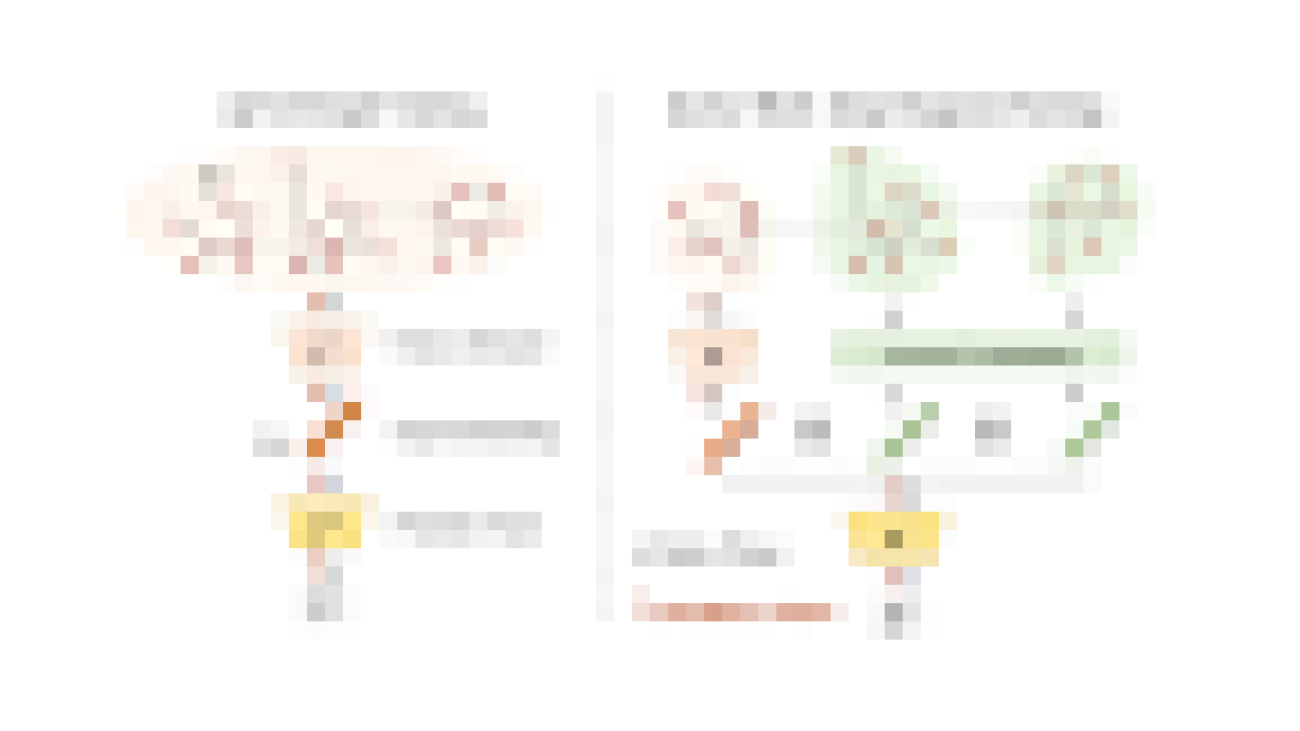
Our algorithm is built by extending standard DP-SGD with an extra mechanism at each iteration to privately select the “hot features”, which are the features that are activated by multiple training examples in the current mini-batch. As illustrated below, the mechanism works in a few steps:
 |
| Illustration of the process of the algorithm on a synthetic categorical feature that has 20 buckets. We compute the number of examples contributing to each bucket, adjust the value based on per-example total contributions (including those to other features), add Gaussian noise, and retain only those buckets with a noisy contribution exceeding the threshold for (noisy) gradient update. |
We provide the theoretical motivation that underlies DP-AdaFEST by viewing it as optimization using stochastic gradient oracles. Standard analysis of stochastic gradient descent in a theoretical setting decomposes the test error of the model into “bias” and “variance” terms. The advantage of DP-AdaFEST can be viewed as reducing variance at the cost of slightly increasing the bias. This is because DP-AdaFEST adds noise to a smaller set of coordinates compared to DP-SGD, which adds noise to all the coordinates. On the other hand, DP-AdaFEST introduces some bias to the gradients since the gradient on the embedding features are dropped with some probability. We refer the interested reader to Section 3.4 of the paper for more details.
We evaluate the effectiveness of our algorithm with large embedding model applications, on public datasets, including one ad prediction dataset (Criteo-Kaggle) and one language understanding dataset (SST-2). We use DP-SGD with exponential selection as a baseline comparison.
The effectiveness of DP-AdaFEST is evident in the figure below, where it achieves significantly higher gradient size reduction (i.e., gradient sparsity) than the baseline while maintaining the same level of utility (i.e., only minimal performance degradation).
Specifically, on the Criteo-Kaggle dataset, DP-AdaFEST reduces the gradient computation cost of regular DP-SGD by more than 5×10⁵ times while maintaining a comparable AUC (which we define as a loss of less than 0.005). This reduction translates into a more efficient and cost-effective training process. In comparison, as shown by the green line below, the baseline method is not able to achieve reasonable cost reduction within such a small utility loss threshold.
In language tasks, there isn’t as much potential for reducing the size of gradients, because the vocabulary used is often smaller and already quite compact (shown on the right below). However, the adoption of sparsity-preserving DP-SGD effectively obviates the dense gradient computation. Furthermore, in line with the bias-variance trade-off presented in the theoretical analysis, we note that DP-AdaFEST occasionally exhibits superior utility compared to DP-SGD when the reduction in gradient size is minimal. Conversely, when incorporating sparsity, the baseline algorithm faces challenges in maintaining utility.
 |
| A comparison of the best gradient size reduction (the ratio of the non-zero gradient value counts between regular DP-SGD and sparsity-preserving algorithms) achieved under ε =1.0 by DP-AdaFEST (our algorithm) and the baseline algorithm (DP-SGD with exponential selection) compared to DP-SGD at different thresholds for utility difference. A higher curve indicates a better utility/efficiency trade-off. |
In practice, most ad prediction models are being continuously trained and evaluated. To simulate this online learning setup, we also evaluate with time-series data, which are notoriously challenging due to being non-stationary. Our evaluation uses the Criteo-1TB dataset, which comprises real-world user-click data collected over 24 days. Consistently, DP-AdaFEST reduces the gradient computation cost of regular DP-SGD by more than 104 times while maintaining a comparable AUC.
 |
| A comparison of the best gradient size reduction achieved under ε =1.0 by DP-AdaFEST (our algorithm) and DP-SGD with exponential selection (a previous algorithm) compared to DP-SGD at different thresholds for utility difference. A higher curve indicates a better utility/efficiency trade-off. DP-AdaFEST consistently outperforms the previous method. |
We present a new algorithm, DP-AdaFEST, for preserving gradient sparsity in differentially private training — particularly in applications involving large embedding models, a fundamental tool for various applications in recommendation systems and natural language processing. Our algorithm achieves significant reductions in gradient size while maintaining accuracy on real-world benchmark datasets. Moreover, it offers flexible options for balancing utility and efficiency via sparsity-controlling parameters, while our proposals offer much better privacy-utility loss.
This work was a collaboration with Badih Ghazi, Pritish Kamath, Ravi Kumar, Pasin Manurangsi and Amer Sinha.

 Now available in the U.S., NotebookLM has new features to help you easily read, take notes and organize your writing projects.Read More
As virtual reality (VR) and augmented reality (AR) technologies continue to grow in popularity, virtual avatars are becoming an increasingly important part of our digital interactions. In particular, virtual avatars are at the center of many social VR and AR interactions, as they are key to representing remote participants and facilitating collaboration.
In the last decade, interdisciplinary scientists have dedicated a significant amount of effort to better understand the use of avatars, and have made many interesting observations, including the capacity of the users to embody their avatar (i.e., the illusion that the avatar body is their own) and the self-avatar follower effect, which creates a binding between the actions of the avatar and the user strong enough that the avatar can actually affect user behavior.
The use of avatars in experiments isn’t just about how users will interact and behave in VR spaces, but also about discovering the limits of human perception and neuroscience. In fact, some VR social experiments often rely on recreating scenarios that can’t be reproduced easily in the real world, such as bar crawls to explore ingroup vs. outgroup effects, or deception experiments, such as the Milgram obedience to authority inside virtual reality. Other studies try to explore deep neuroscientific phenomena, like the human mechanisms for motor control. This perhaps follows the trail of the rubber hand illusion on brain plasticity, where a person can start feeling as if they own a rubber hand while their real hand is hidden behind a curtain. There is also an increased number of possible therapies for psychiatric treatment using personalized avatars. In these cases, VR becomes an ecologically valid tool that allows scientists to explore or treat human behavior and perception.
None of these experiments and therapies could exist without good access to research tools and libraries that can enable easy experimentation. As such, multiple systems and open source tools have been released around avatar creation and animation over recent years. However, existing avatar libraries have not been validated systematically on the diversity spectrum. Societal bias and dynamics also transfer to VR/AR when interacting with avatars, which could lead to incomplete conclusions for studies on human behavior inside VR/AR.
To partially overcome this problem, we partnered with the University of Central Florida to create and release the open-source Virtual Avatar Library for Inclusion and Diversity (VALID). Described in our recent paper, published in Frontiers in Virtual Reality, this library of avatars is readily available for usage in VR/AR experiments and includes 210 avatars of seven different races and ethnicities recognized by the US Census Bureau. The avatars have been perceptually validated and designed to advance diversity and inclusion in virtual avatar research.
 |
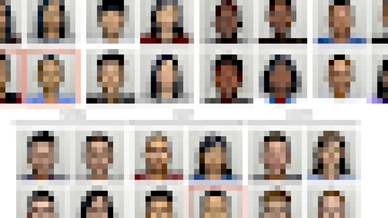
| Headshots of all 42 base avatars available on the VALID library were created in extensive interaction with members of the 7 ethnic and racial groups from the Federal Register, which include (AIAN, Asian, Black, Hispanic, MENA, NHPI and White). |
Our initial selection of races and ethnicities for the diverse avatar library follows the most recent guidelines of the US Census Bureau that as of 2023 recommended the use of 7 ethnic and racial groups representing a large demographic of the US society, which can also be extrapolated to the global population. These groups include Hispanic or Latino, American Indian or Alaska Native (AIAN), Asian, Black or African American, Native Hawaiian or Other Pacific Islander (NHPI), White, Middle East or North Africa (MENA). We envision the library will continue to evolve to bring even more diversity and representation with future additions of avatars.
The avatars were hand modeled and created using a process that combined average facial features with extensive collaboration with representative stakeholders from each racial group, where their feedback was used to artistically modify the facial mesh of the avatars. Then we conducted an online study with participants from 33 countries to determine whether the race and gender of each avatar in the library are recognizable. In addition to the avatars, we also provide labels statistically validated through observation of users for the race and gender of all 42 base avatars (see below).
 |
| Example of the headshots of a Black/African American avatar presented to participants during the validation of the library. |
We found that all Asian, Black, and White avatars were universally identified as their modeled race by all participants, while our American Indian or Native Alaskan (AIAN), Hispanic, and Middle Eastern or North African (MENA) avatars were typically only identified by participants of the same race. This also indicates that participant race can improve identification of a virtual avatar of the same race. The paper accompanying the library release highlights how this ingroup familiarity should also be taken into account when studying avatar behavior in VR.
 |
| Confusion matrix heatmap of agreement rates for the 42 base avatars separated by other-race participants and same-race participants. One interesting aspect visible in this matrix, is that participants were significantly better at identifying the avatars of their own race than other races. |
Our models are available in FBX format, are compatible with previous avatar libraries like the commonly used Rocketbox, and can be easily integrated into most game engines such as Unity and Unreal. Additionally, the avatars come with 69 bones and 65 facial blendshapes to enable researchers and developers to easily create and apply dynamic facial expressions and animations. The avatars were intentionally made to be partially cartoonish to avoid extreme look-a-like scenarios in which a person could be impersonated, but still representative enough to be able to run reliable user studies and social experiments.
 |
| Images of the skeleton rigging (bones that allow for animation) and some facial blend shapes included with the VALID avatars. |
The avatars can be further combined with variations of casual attires and five professional attires, including medical, military, worker and business. This is an intentional improvement from prior libraries that in some cases reproduced stereotypical gender and racial bias into the avatar attires, and provided very limited diversity to certain professional avatars.
 |
| Images of some sample attire included with the VALID avatars. |
We believe that the Virtual Avatar Library for Inclusion and Diversity (VALID) will be a valuable resource for researchers and developers working on VR/AR applications. We hope it will help to create more inclusive and equitable virtual experiences. To this end, we invite you to explore the avatar library, which we have released under the open source MIT license. You can download the avatars and use them in a variety of settings at no charge.
This library of avatars was born out of a collaboration with Tiffany D. Do, Steve Zelenty and Prof. Ryan P McMahan from the University of Central Florida.