
Caching is a ubiquitous idea in computer science that significantly improves the performance of storage and retrieval systems by storing a subset of popular items closer to the client based on request patterns. An important algorithmic piece of cache management is the decision policy used for dynamically updating the set of items being stored, which has been extensively optimized over several decades, resulting in several efficient and robust heuristics. While applying machine learning to cache policies has shown promising results in recent years (e.g., LRB, LHD, storage applications), it remains a challenge to outperform robust heuristics in a way that can generalize reliably beyond benchmarks to production settings, while maintaining competitive compute and memory overheads.
In “HALP: Heuristic Aided Learned Preference Eviction Policy for YouTube Content Delivery Network”, presented at NSDI 2023, we introduce a scalable state-of-the-art cache eviction framework that is based on learned rewards and uses preference learning with automated feedback. The Heuristic Aided Learned Preference (HALP) framework is a meta-algorithm that uses randomization to merge a lightweight heuristic baseline eviction rule with a learned reward model. The reward model is a lightweight neural network that is continuously trained with ongoing automated feedback on preference comparisons designed to mimic the offline oracle. We discuss how HALP has improved infrastructure efficiency and user video playback latency for YouTube’s content delivery network.
Learned preferences for cache eviction decisions
The HALP framework computes cache eviction decisions based on two components: (1) a neural reward model trained with automated feedback via preference learning, and (2) a meta-algorithm that combines a learned reward model with a fast heuristic. As the cache observes incoming requests, HALP continuously trains a small neural network that predicts a scalar reward for each item by formulating this as a preference learning method via pairwise preference feedback. This aspect of HALP is similar to reinforcement learning from human feedback (RLHF) systems, but with two important distinctions:
- Feedback is automated and leverages well-known results about the structure of offline optimal cache eviction policies.
- The model is learned continuously using a transient buffer of training examples constructed from the automated feedback process.
The eviction decisions rely on a filtering mechanism with two steps. First, a small subset of candidates is selected using a heuristic that is efficient, but suboptimal in terms of performance. Then, a re-ranking step optimizes from within the baseline candidates via the sparing use of a neural network scoring function to “boost” the quality of the final decision.
As a production ready cache policy implementation, HALP not only makes eviction decisions, but also subsumes the end-to-end process of sampling pairwise preference queries used to efficiently construct relevant feedback and update the model to power eviction decisions.
A neural reward model
HALP uses a light-weight two-layer multilayer perceptron (MLP) as its reward model to selectively score individual items in the cache. The features are constructed and managed as a metadata-only “ghost cache” (similar to classical policies like ARC). After any given lookup request, in addition to regular cache operations, HALP conducts the book-keeping (e.g., tracking and updating feature metadata in a capacity-constrained key-value store) needed to update the dynamic internal representation. This includes: (1) externally tagged features provided by the user as input, along with a cache lookup request, and (2) internally constructed dynamic features (e.g., time since last access, average time between accesses) constructed from lookup times observed on each item.
HALP learns its reward model fully online starting from a random weight initialization. This might seem like a bad idea, especially if the decisions are made exclusively for optimizing the reward model. However, the eviction decisions rely on both the learned reward model and a suboptimal but simple and robust heuristic like LRU. This allows for optimal performance when the reward model has fully generalized, while remaining robust to a temporarily uninformative reward model that is yet to generalize, or in the process of catching up to a changing environment.
Another advantage of online training is specialization. Each cache server runs in a potentially different environment (e.g., geographic location), which influences local network conditions and what content is locally popular, among other things. Online training automatically captures this information while reducing the burden of generalization, as opposed to a single offline training solution.
Scoring samples from a randomized priority queue
It can be impractical to optimize for the quality of eviction decisions with an exclusively learned objective for two reasons.
- Compute efficiency constraints: Inference with a learned network can be significantly more expensive than the computations performed in practical cache policies operating at scale. This limits not only the expressivity of the network and features, but also how often these are invoked during each eviction decision.
- Robustness for generalizing out-of-distribution: HALP is deployed in a setup that involves continual learning, where a quickly changing workload might generate request patterns that might be temporarily out-of-distribution with respect to previously seen data.
To address these issues, HALP first applies an inexpensive heuristic scoring rule that corresponds to an eviction priority to identify a small candidate sample. This process is based on efficient random sampling that approximates exact priority queues. The priority function for generating candidate samples is intended to be quick to compute using existing manually-tuned algorithms, e.g., LRU. However, this is configurable to approximate other cache replacement heuristics by editing a simple cost function. Unlike prior work, where the randomization was used to tradeoff approximation for efficiency, HALP also relies on the inherent randomization in the sampled candidates across time steps for providing the necessary exploratory diversity in the sampled candidates for both training and inference.
The final evicted item is chosen from among the supplied candidates, equivalent to the best-of-n reranked sample, corresponding to maximizing the predicted preference score according to the neural reward model. The same pool of candidates used for eviction decisions is also used to construct the pairwise preference queries for automated feedback, which helps minimize the training and inference skew between samples.
 |
| An overview of the two-stage process invoked for each eviction decision. |
Online preference learning with automated feedback
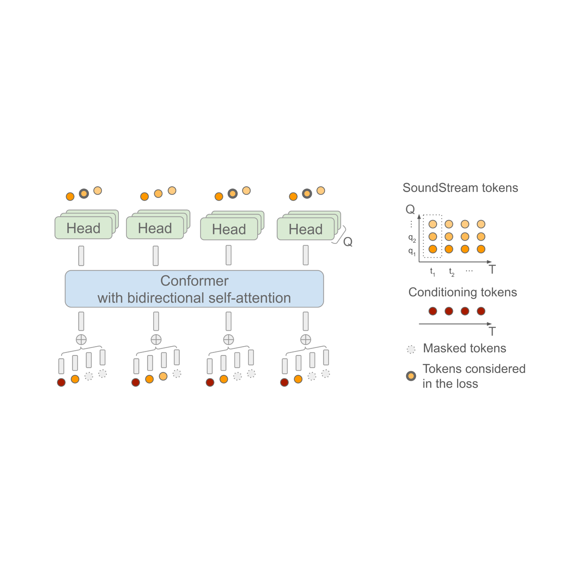
The reward model is learned using online feedback, which is based on automatically assigned preference labels that indicate, wherever feasible, the ranked preference ordering for the time taken to receive future re-accesses, starting from a given snapshot in time among each queried sample of items. This is similar to the oracle optimal policy, which, at any given time, evicts an item with the farthest future access from all the items in the cache.
 |
| Generation of the automated feedback for learning the reward model. |
To make this feedback process informative, HALP constructs pairwise preference queries that are most likely to be relevant for eviction decisions. In sync with the usual cache operations, HALP issues a small number of pairwise preference queries while making each eviction decision, and appends them to a set of pending comparisons. The labels for these pending comparisons can only be resolved at a random future time. To operate online, HALP also performs some additional book-keeping after each lookup request to process any pending comparisons that can be labeled incrementally after the current request. HALP indexes the pending comparison buffer with each element involved in the comparison, and recycles the memory consumed by stale comparisons (neither of which may ever get a re-access) to ensure that the memory overhead associated with feedback generation remains bounded over time.
 |
| Overview of all main components in HALP. |
Results: Impact on the YouTube CDN
Through empirical analysis, we show that HALP compares favorably to state-of-the-art cache policies on public benchmark traces in terms of cache miss rates. However, while public benchmarks are a useful tool, they are rarely sufficient to capture all the usage patterns across the world over time, not to mention the diverse hardware configurations that we have already deployed.
Until recently, YouTube servers used an optimized LRU-variant for memory cache eviction. HALP increases YouTube’s memory egress/ingress — the ratio of the total bandwidth egress served by the CDN to that consumed for retrieval (ingress) due to cache misses — by roughly 12% and memory hit rate by 6%. This reduces latency for users, since memory reads are faster than disk reads, and also improves egressing capacity for disk-bounded machines by shielding the disks from traffic.
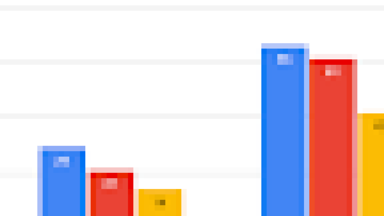
The figure below shows a visually compelling reduction in the byte miss ratio in the days following HALP’s final rollout on the YouTube CDN, which is now serving significantly more content from within the cache with lower latency to the end user, and without having to resort to more expensive retrieval that increases the operating costs.
 |
| Aggregate worldwide YouTube byte miss ratio before and after rollout (vertical dashed line). |
An aggregated performance improvement could still hide important regressions. In addition to measuring overall impact, we also conduct an analysis in the paper to understand its impact on different racks using a machine level analysis, and find it to be overwhelmingly positive.
Conclusion
We introduced a scalable state-of-the-art cache eviction framework that is based on learned rewards and uses preference learning with automated feedback. Because of its design choices, HALP can be deployed in a manner similar to any other cache policy without the operational overhead of having to separately manage the labeled examples, training procedure and the model versions as additional offline pipelines common to most machine learning systems. Therefore, it incurs only a small extra overhead compared to other classical algorithms, but has the added benefit of being able to take advantage of additional features to make its eviction decisions and continuously adapt to changing access patterns.
This is the first large-scale deployment of a learned cache policy to a widely used and heavily trafficked CDN, and has significantly improved the CDN infrastructure efficiency while also delivering a better quality of experience to users.
Acknowledgements
Ramki Gummadi is now part of Google DeepMind. We would like to thank John Guilyard for help with the illustrations and Richard Schooler for feedback on this post.

 Google’s Yossi Matias and WMO Director of Infrastructure Anthony Rea discuss the Early Warnings For All Initiative.
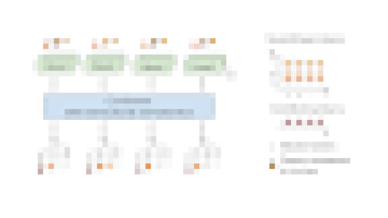


 This 10-week program supports startups using AI in their core business through tailored training and mentoring by making use of the best of Google and its network.
 James Manyika spoke at the Cannes Lions Festival about AI and creativity. Read excerpts from his remarks.


 Lens makes it easy to search what you see and explore the world around you — including the new ability to search for skin conditions.