Posts in category: Google AI

Posted by Bowen Zhang, Student Researcher and Jiahui Yu, Senior Research Scientist, Google Research, Brain Team

Action recognition has become a major focus area for the research community because many applications can benefit from improved modeling, such as video retrieval, video captioning, video question-answering, etc. Transformer-based approaches have recently demonstrated state-of-the-art performance on several benchmarks. While Transformer models require data to learn better visual priors compared to ConvNets, action recognition datasets are relatively small in scale. Large Transformer models are typically first trained on image datasets and later fine-tuned on a target action recognition dataset.

While the current pre-training and fine-tuning action recognition paradigm is straightforward and manifests strong empirical results, it may be overly restrictive for building general-purpose action-recognition models. Compared to a dataset like ImageNet that covers a large range of object recognition classes, action recognition datasets like Kinetics and Something-Something-v2 (SSv2) pertain to limited topics. For example, Kinetics include object-centric actions like “cliff diving” and “ice climbing’ while SSv2 contains object-agnostic activities like ’pretending to put something onto something else.’ As a result, we observed poor performance adapting an action recognition model that has been fine-tuned on one dataset to another disparate dataset.

Differences in objects and video backgrounds among datasets further exacerbate learning a general-purpose action recognition classification model. Despite the fact that video datasets may be increasing in size, prior work suggests significant data augmentation and regularization is necessary to achieve strong performance. This latter finding may indicate the model quickly overfits on the target dataset, and as a result, hinders its capacity to generalize to other action recognition tasks.

In “Co-training Transformer with Videos and Images Improves Action Recognition”, we propose a training strategy, named CoVeR, that leverages both image and video data to jointly learn a single general-purpose action recognition model. Our approach is buttressed by two main findings. First, disparate video datasets cover a diverse set of activities, and training them together in a single model could lead to a model that excels at a wide range of activities. Second, video is a perfect source for learning motion information, while images are great for exploiting structural appearance. Leveraging a diverse distribution of image examples may be beneficial in building robust spatial representations in video models. Concretely, CoVeR first pre-trains the model on an image dataset, and during fine-tuning, it simultaneously trains a single model on multiple video and image datasets to build robust spatial and temporal representations for a general-purpose video understanding model.

Architecture and Training Strategy
We applied the CoVeR approach to the recently proposed spatial-temporal video transformer, called TimeSFormer, that contains 24 layers of transformer blocks. Each block contains one temporal attention, one spatial attention, and one multilayer perceptron (MLP) layer. To learn from multiple video and image datasets, we adopt a multi-task learning paradigm and equip the action recognition model with multiple classification heads. We pre-train all non-temporal parameters on the large-scale JFT dataset. During fine-tuning, a batch of videos and images are sampled from multiple video and image datasets. The sampling rate is proportional to the size of the datasets. Each sample within the batch is processed by the TimeSFormer and then distributed to the corresponding classifier to get the predictions.

Compared with the standard training strategy, CoVeR has two advantages. First, as the model is directly trained on multiple datasets, the learned video representations are more general and can be directly evaluated on those datasets without additional fine-tuning. Second, Transformer-based models may easily overfit to a smaller video distribution, thus degrading the generalization of the learned representations. Training on multiple datasets mitigates this challenge by reducing the risk of overfitting.

CoVeR adopts a multi-task learning strategy trained on multiple datasets, each with their own classifier.

Benchmark Results
We evaluate the CoVeR approach to train on Kinetics-400 (K400), Kinetics-600 (K600), Kinetics-700 (K700), SomethingSomething-V2 (SSv2), and Moments-in-Time (MiT) datasets. Compared with other approaches — such as TimeSFormer, Video SwinTransformer, TokenLearner, ViViT, MoViNet, VATT, VidTr, and OmniSource — CoVeR established the new state-of-the-art on multiple datasets (shown below). Unlike previous approaches that train a dedicated model for one single dataset, a model trained by CoVeR can be directly applied to multiple datasets without further fine-tuning.

Transfer Learning
We use transfer learning to further verify the video action recognition performance and compare with co-training on multiple datasets, results are summarized below. Specifically, we train on the source datasets, then fine-tune and evaluate on the target dataset.

We first consider K400 as the target dataset. CoVeR co-trained on SSv2 and MiT improves the top-1 accuracy on K400→K400 (where the model is trained on K400 and then fine-tuned on K400) by 1.3%, SSv2→K400 by 1.7%, and MiT→K400 by 0.4%. Similarly, we observe that by transferring to SSv2, CoVeR achieves 2%, 1.8%, and 1.1% improvement over SSv2→SSv2, K400→SSv2, and MiT→SSv2, respectively. The 1.2% and 2% performance improvement on K400 and SSv2 indicates that CoVeR co-trained on multiple datasets could learn better visual representations than the standard training paradigm, which is useful for downstream tasks.

Comparison of transfer learning the representation learned by CoVeR and standard training paradigm. A→B means the model is trained on dataset A and then fine-tuned on dataset B.

Conclusion
In this work, we present CoVeR, a training paradigm that jointly learns action recognition and object recognition tasks in a single model for the purpose of constructing a general-purpose action recognition framework. Our analysis indicates that it may be beneficial to integrate many video datasets into one multi-task learning paradigm. We highlight the importance of continuing to learn on image data during fine-tuning to maintain robust spatial representations. Our empirical findings suggest CoVeR can learn a single general-purpose video understanding model which achieves impressive performance across many action recognition datasets without an additional stage of fine-tuning on each downstream application.

Acknowledgements
We would like to thank Christopher Fifty, Wei Han, Andrew M. Dai, Ruoming Pang, and Fei Sha for preparation of the CoVeR paper, Yue Zhao, Hexiang Hu, Zirui Wang, Zitian Chen, Qingqing Huang, Claire Cui and Yonghui Wu for helpful discussions and feedbacks, and others on the Brain Team for support throughout this project.

Read More

Posted by Brendan McMahan and Abhradeep Thakurta, Research Scientists, Google Research

In 2017, Google introduced federated learning (FL), an approach that enables mobile devices to collaboratively train machine learning (ML) models while keeping the raw training data on each user’s device, decoupling the ability to do ML from the need to store the data in the cloud. Since its introduction, Google has continued to actively engage in FL research and deployed FL to power many features in Gboard, including next word prediction, emoji suggestion and out-of-vocabulary word discovery. Federated learning is improving the “Hey Google” detection models in Assistant, suggesting replies in Google Messages, predicting text selections, and more.

While FL allows ML without raw data collection, differential privacy (DP) provides a quantifiable measure of data anonymization, and when applied to ML can address concerns about models memorizing sensitive user data. This too has been a top research priority, and has yielded one of the first production uses of DP for analytics with RAPPOR in 2014, our open-source DP library, Pipeline DP, and TensorFlow Privacy.

Through a multi-year, multi-team effort spanning fundamental research and product integration, today we are excited to announce that we have deployed a production ML model using federated learning with a rigorous differential privacy guarantee. For this proof-of-concept deployment, we utilized the DP-FTRL algorithm to train a recurrent neural network to power next-word-prediction for Spanish-language Gboard users. To our knowledge, this is the first production neural network trained directly on user data announced with a formal DP guarantee (technically ρ=0.81 zero-Concentrated-Differential-Privacy, zCDP, discussed in detail below). Further, the federated approach offers complimentary data minimization advantages, and the DP guarantee protects all of the data on each device, not just individual training examples.

Data Minimization and Anonymization in Federated Learning
Along with fundamentals like transparency and consent, the privacy principles of data minimization and anonymization are important in ML applications that involve sensitive data.

Federated learning systems structurally incorporate the principle of data minimization. FL only transmits minimal updates for a specific model training task (focused collection), limits access to data at all stages, processes individuals’ data as early as possible (early aggregation), and discards both collected and processed data as soon as possible (minimal retention).

Another principle that is important for models trained on user data is anonymization, meaning that the final model should not memorize information unique to a particular individual’s data, e.g., phone numbers, addresses, credit card numbers. However, FL on its own does not directly tackle this problem.

The mathematical concept of DP allows one to formally quantify this principle of anonymization. Differentially private training algorithms add random noise during training to produce a probability distribution over output models, and ensure that this distribution doesn’t change too much given a small change to the training data; ρ-zCDP quantifies how much the distribution could possibly change. We call this example-level DP when adding or removing a single training example changes the output distribution on models in a provably minimal way.

Showing that deep learning with example-level differential privacy was even possible in the simpler setting of centralized training was a major step forward in 2016. Achieved by the DP-SGD algorithm, the key was amplifying the privacy guarantee by leveraging the randomness in sampling training examples (“amplification-via-sampling”).

However, when users can contribute multiple examples to the training dataset, example-level DP is not necessarily strong enough to ensure the users’ data isn’t memorized. Instead, we have designed algorithms for user-level DP, which requires that the output distribution of models doesn’t change even if we add/remove all of the training examples from any one user (or all the examples from any one device in our application). Fortunately, because FL summarizes all of a user’s training data as a single model update, federated algorithms are well-suited to offering user-level DP guarantees.

Both limiting the contributions from one user and adding noise can come at the expense of model accuracy, however, so maintaining model quality while also providing strong DP guarantees is a key research focus.

The Challenging Path to Federated Learning with Differential Privacy
In 2018, we introduced the DP-FedAvg algorithm, which extended the DP-SGD approach to the federated setting with user-level DP guarantees, and in 2020 we deployed this algorithm to mobile devices for the first time. This approach ensures the training mechanism is not too sensitive to any one user’s data, and empirical privacy auditing techniques rule out some forms of memorization.

However, the amplification-via-samping argument is essential to providing a strong DP guarantee for DP-FedAvg, but in a real-world cross-device FL system ensuring devices are subsampled precisely and uniformly at random from a large population would be complex and hard to verify. One challenge is that devices choose when to connect (or “check in”) based on many external factors (e.g., requiring the device is idle, on unmetered WiFi, and charging), and the number of available devices can vary substantially.

Achieving a formal privacy guarantee requires a protocol that does all of the following:

• Makes progress on training even as the set of devices available varies significantly with time.
• Maintains privacy guarantees even in the face of unexpected or arbitrary changes in device availability.
• For efficiency, allows client devices to locally decide whether they will check in to the server in order to participate in training, independent of other devices.

Initial work on privacy amplification via random check-ins highlighted these challenges and introduced a feasible protocol, but it would have required complex changes to our production infrastructure to deploy. Further, as with the amplification-via-sampling analysis of DP-SGD, the privacy amplification possible with random check-ins depends on a large number of devices being available. For example, if only 1000 devices are available for training, and participation of at least 1000 devices is needed in each training step, that requires either 1) including all devices currently available and paying a large privacy cost since there is no randomness in the selection, or 2) pausing the protocol and not making progress until more devices are available.

Achieving Provable Differential Privacy for Federated Learning with DP-FTRL
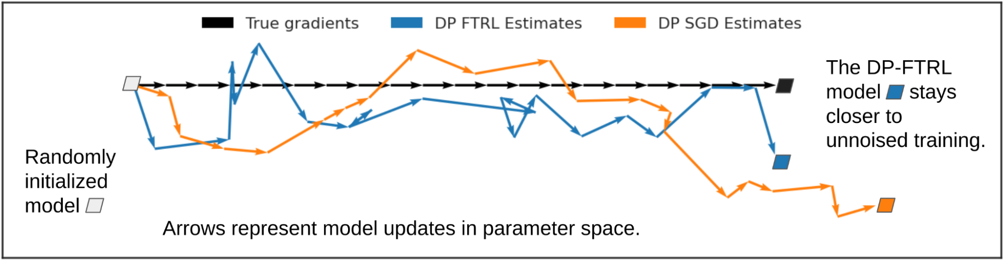
To address this challenge, the DP-FTRL algorithm is built on two key observations: 1) the convergence of gradient-descent-style algorithms depends primarily not on the accuracy of individual gradients, but the accuracy of cumulative sums of gradients; and 2) we can provide accurate estimates of cumulative sums with a strong DP guarantee by utilizing negatively correlated noise, added by the aggregating server: essentially, adding noise to one gradient and subtracting that same noise from a later gradient. DP-FTRL accomplishes this efficiently using the Tree Aggregation algorithm [1, 2].

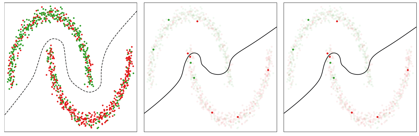
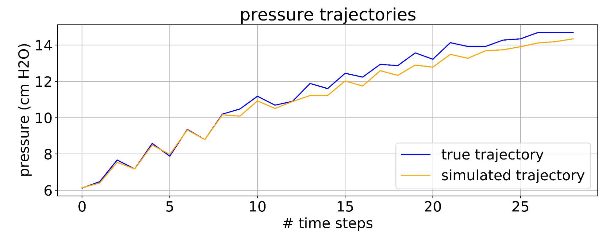
The graphic below illustrates how estimating cumulative sums rather than individual gradients can help. We look at how the noise introduced by DP-FTRL and DP-SGD influence model training, compared to the true gradients (without added noise; in black) which step one unit to the right on each iteration. The individual DP-FTRL gradient estimates (blue), based on cumulative sums, have larger mean-squared-error than the individually-noised DP-SGD estimates (orange), but because the DP-FTRL noise is negatively correlated, some of it cancels out from step to step, and the overall learning trajectory stays closer to the true gradient descent steps.

To provide a strong privacy guarantee, we limit the number of times a user contributes an update. Fortunately, sampling-without-replacement is relatively easy to implement in production FL infrastructure: each device can remember locally which models it has contributed to in the past, and choose to not connect to the server for any later rounds for those models.

Production Training Details and Formal DP Statements
For the production DP-FTRL deployment introduced above, each eligible device maintains a local training cache consisting of user keyboard input, and when participating computes an update to the model which makes it more likely to suggest the next word the user actually typed, based on what has been typed so far. We ran DP-FTRL on this data to train a recurrent neural network with ~1.3M parameters. Training ran for 2000 rounds over six days, with 6500 devices participating per round. To allow for the DP guarantee, devices participated in training at most once every 24 hours. Model quality improved over the previous DP-FedAvg trained model, which offered empirically-tested privacy advantages over non-DP models, but lacked a meaningful formal DP guarantee.

The training mechanism we used is available in open-source in TensorFlow Federated and TensorFlow Privacy, and with the parameters used in our production deployment it provides a meaningfully strong privacy guarantee. Our analysis gives ρ=0.81 zCDP at the user level (treating all the data on each device as a different user), where smaller numbers correspond to better privacy in a mathematically precise way. As a comparison, this is stronger than the ρ=2.63 zCDP guarantee chosen by the 2020 US Census.

Next Steps
While we have reached the milestone of deploying a production FL model using a mechanism that provides a meaningfully small zCDP, our research journey continues. We are still far from being able to say this approach is possible (let alone practical) for most ML models or product applications, and other approaches to private ML exist. For example, membership inference tests and other empirical privacy auditing techniques can provide complimentary safeguards against leakage of users’ data. Most importantly, we see training models with user-level DP with even a very large zCDP as a substantial step forward, because it requires training with a DP mechanism that bounds the sensitivity of the model to any one user’s data. Further, it smooths the road to later training models with improved privacy guarantees as better algorithms or more data become available. We are excited to continue the journey toward maximizing the value that ML can deliver while minimizing potential privacy costs to those who contribute training data.

Acknowledgements
The authors would like to thank Alex Ingerman and Om Thakkar for significant impact on the blog post itself, as well as the teams at Google that helped develop these ideas and bring them to practice:

• Core research team: Galen Andrew, Borja Balle, Peter Kairouz, Daniel Ramage, Shuang Song, Thomas Steinke, Andreas Terzis, Om Thakkar, Zheng Xu
• FL infrastructure team: Katharine Daly, Stefan Dierauf, Hubert Eichner, Igor Pisarev, Timon Van Overveldt, Chunxiang Zheng
• Gboard team: Angana Ghosh, Xu Liu, Yuanbo Zhang
• Speech team: Françoise Beaufays, Mingqing Chen, Rajiv Mathews, Vidush Mukund, Igor Pisarev, Swaroop Ramaswamy, Dan Zivkovic

Read More

Posted by Abhishek Kumar and Ehsan Amid, Research Scientists, Google Research, Brain Team

Over the past several years, deep neural networks (DNNs) have been quite successful in driving impressive performance gains in several real-world applications, from image recognition to genomics. However, modern DNNs often have far more trainable model parameters than the number of training examples and the resulting overparameterized networks can easily overfit to noisy or corrupted labels (i.e., examples that are assigned a wrong class label). As a consequence, training with noisy labels often leads to degradation in accuracy of the trained model on clean test data. Unfortunately, noisy labels can appear in several real-world scenarios due to multiple factors, such as errors and inconsistencies in manual annotation and the use of inherently noisy label sources (e.g., the internet or automated labels from an existing system).

Earlier work has shown that representations learned by pre-training large models with noisy data can be useful for prediction when used in a linear classifier trained with clean data. In principle, it is possible to directly train machine learning (ML) models on noisy data without resorting to this two-stage approach. To be successful, such alternative methods should have the following properties: (i) they should fit easily into standard training pipelines with little computational or memory overhead; (ii) they should be applicable in “streaming” settings where new data is continuously added during training; and (iii) they should not require data with clean labels.

In “Constrained Instance and Class Reweighting for Robust Learning under Label Noise”, we propose a novel and principled method, named Constrained Instance reWeighting (CIW), with these properties that works by dynamically assigning importance weights both to individual instances and to class labels in a mini-batch, with the goal of reducing the effect of potentially noisy examples. We formulate a family of constrained optimization problems that yield simple solutions for these importance weights. These optimization problems are solved per mini-batch, which avoids the need to store and update the importance weights over the full dataset. This optimization framework also provides a theoretical perspective for existing label smoothing heuristics that address label noise, such as label bootstrapping. We evaluate the method with varying amounts of synthetic noise on the standard CIFAR-10 and CIFAR-100 benchmarks and observe considerable performance gains over several existing methods.

Method
Training ML models involves minimizing a loss function that indicates how well the current parameters fit to the given training data. In each training step, this loss is approximately calculated as a (weighted) sum of the losses of individual instances in the mini-batch of data on which it is operating. In standard training, each instance is treated equally for the purpose of updating the model parameters, which corresponds to assigning uniform (i.e., equal) weights across the mini-batch.

However, empirical observations made in earlier works reveal that noisy or mislabeled instances tend to have higher loss values than those that are clean, particularly during early to mid-stages of training. Thus, assigning uniform importance weights to all instances means that due to their higher loss values, the noisy instances can potentially dominate the clean instances and degrade the accuracy on clean test data.

Motivated by these observations, we propose a family of constrained optimization problems that solve this problem by assigning importance weights to individual instances in the dataset to reduce the effect of those that are likely to be noisy. This approach provides control over how much the weights deviate from uniform, as quantified by a divergence measure. It turns out that for several types of divergence measures, one can obtain simple formulae for the instance weights. The final loss is computed as the weighted sum of individual instance losses, which is used for updating the model parameters. We call this the Constrained Instance reWeighting (CIW) method. This method allows for controlling the smoothness or peakiness of the weights through the choice of divergence and a corresponding hyperparameter.

Schematic of the proposed Constrained Instance reWeighting (CIW) method.

Illustration with Decision Boundary on a 2D Dataset
As an example to illustrate the behavior of this method, we consider a noisy version of the Two Moons dataset, which consists of randomly sampled points from two classes in the shape of two half moons. We corrupt 30% of the labels and train a multilayer perceptron network on it for binary classification. We use the standard binary cross-entropy loss and an SGD with momentum optimizer to train the model. In the figure below (left panel), we show the data points and visualize an acceptable decision boundary separating the two classes with a dotted line. The points marked red in the upper half-moon and those marked green in the lower half-moon indicate noisy data points.

The baseline model trained with the binary cross-entropy loss assigns uniform weights to the instances in each mini-batch, thus eventually overfitting to the noisy instances and resulting in a poor decision boundary (middle panel in the figure below).

The CIW method reweights the instances in each mini-batch based on their corresponding loss values (right panel in the figure below). It assigns larger weights to the clean instances that are located on the correct side of the decision boundary and damps the effect of noisy instances that incur a higher loss value. Smaller weights for noisy instances help in preventing the model from overfitting to them, thus allowing the model trained with CIW to successfully converge to a good decision boundary by avoiding the impact of label noise.

Illustration of decision boundary as the training proceeds for the baseline and the proposed CIW method on the Two Moons dataset. Left: Noisy dataset with a desirable decision boundary. Middle: Decision boundary for standard training with cross-entropy loss. Right: Training with the CIW method. The size of the dots in (middle) and (right) are proportional to the importance weights assigned to these examples in the minibatch.

<!–

–>

Constrained Class reWeighting
Instance reweighting assigns lower weights to instances with higher losses. We further extend this intuition to assign importance weights over all possible class labels. Standard training uses a one-hot label vector as the class weights, assigning a weight of 1 to the labeled class and 0 to all other classes. However, for the potentially mislabeled instances, it is reasonable to assign non-zero weights to classes that could be the true label. We obtain these class weights as solutions to a family of constrained optimization problems where the deviation of the class weights from the label one-hot distribution, as measured by a divergence of choice, is controlled by a hyperparameter.

Again, for several divergence measures, we can obtain simple formulae for the class weights. We refer to this as Constrained Instance and Class reWeighting (CICW). The solution to this optimization problem also recovers the earlier proposed methods based on static label bootstrapping (also referred as label smoothing) when the divergence is taken to be total variation distance. This provides a theoretical perspective on the popular method of static label bootstrapping.

Using Instance Weights with Mixup
We also propose a way to use the obtained instance weights with mixup, which is a popular method for regularizing models and improving prediction performance. It works by sampling a pair of examples from the original dataset and generating a new artificial example using a random convex combination of these. The model is trained by minimizing the loss on these mixed-up data points. Vanilla mixup is oblivious to the individual instance losses, which might be problematic for noisy data because mixup will treat clean and noisy examples equally. Since a high instance weight obtained with our CIW method is more likely to indicate a clean example, we use our instance weights to do a biased sampling for mixup and also use the weights in convex combinations (instead of random convex combinations in vanilla mixup). This results in biasing the mixed-up examples towards clean data points, which we refer to as CICW-Mixup.

We apply these methods with varying amounts of synthetic noise (i.e., the label for each instance is randomly flipped to other labels) on the standard CIFAR-10 and CIFAR-100 benchmark datasets. We show the test accuracy on clean data with symmetric synthetic noise where the noise rate is varied between 0.2 and 0.8.

We observe that the proposed CICW outperforms several methods and matches the results of dynamic mixup, which maintains the importance weights over the full training set with mixup. Using our importance weights with mixup in CICW-M, resulted in significantly improved performance vs these methods, particularly for larger noise rates (as shown by lines above and to the right in the graphs below).

Test accuracy on clean data while varying the amount of symmetric synthetic noise in the training data for CIFAR-10 and CIFAR-100. Methods compared are: standard Cross-Entropy Loss (CE), Bi-tempered Loss, Active-Passive Normalized Loss, the proposed CICW, Mixup, Dynamic Mixup, and the proposed CICW-Mixup.

Summary and Future Directions
We formulate a novel family of constrained optimization problems for tackling label noise that yield simple mathematical formulae for reweighting the training instances and class labels. These formulations also provide a theoretical perspective on existing label smoothing–based methods for learning with noisy labels. We also propose ways for using the instance weights with mixup that results in further significant performance gains over instance and class reweighting. Our method operates solely at the level of mini-batches, which avoids the extra overhead of maintaining dataset-level weights as in some of the recent methods.

As a direction for future work, we would like to evaluate the method on realistic noisy labels that are encountered in large scale practical settings. We also believe that studying the interaction of our framework with label smoothing is an interesting direction that can result in a loss adaptive version of label smoothing. We are also excited to release the code for CICW, now available on Github.

Acknowledgements
We’d like to thank Kevin Murphy for providing constructive feedback during the course of the project.

Read More

Posted by AJ Piergiovanni and Anelia Angelova, Research Scientists, Google Research

While not immediately obvious, all of us experience the world in four dimensions (4D). For example, when walking or driving down the street we observe a stream of visual inputs, snapshots of the 3D world, which, when taken together in time, creates a 4D visual input. Today’s autonomous vehicles and robots are able to capture much of this information through various onboard sensing mechanisms, such as LiDAR and cameras.

LiDAR is a ubiquitous sensor that uses light pulses to reliably measure the 3D coordinates of objects in a scene, however, it is also sparse and has a limited range — the farther one is from a sensor, the fewer points will be returned. This means that far-away objects might only get a handful of points, or none at all, and might not be seen by LiDAR alone. At the same time, images from the onboard camera, which is a dense input, are incredibly useful for semantic understanding, such as detecting and segmenting objects. With high resolution, cameras can be very effective at detecting objects far away, but are less accurate in measuring the distance.

Autonomous vehicles collect data from both LiDAR and onboard camera sensors. Each sensor measurement is recorded at regular time intervals, providing an accurate representation of the 4D world. However, very few research algorithms use both of these in combination, especially when taken “in time”, i.e., as a temporally ordered sequence of data, mostly due to two major challenges. When using both sensing modalities simultaneously, 1) it is difficult to maintain computational efficiency, and 2) pairing the information from one sensor to another adds further complexity since there is not always a direct correspondence between LiDAR points and onboard camera RGB image inputs.

In “4D-Net for Learned Multi-Modal Alignment”, published at ICCV 2021, we present a neural network that can process 4D data, which we call 4D-Net. This is the first attempt to effectively combine both types of sensors, 3D LiDAR point clouds and onboard camera RGB images, when both are in time. We also introduce a dynamic connection learning method, which incorporates 4D information from a scene by performing connection learning across both feature representations. Finally, we demonstrate that 4D-Net is better able to use motion cues and dense image information to detect distant objects while maintaining computational efficiency.

4D-Net
In our scenario, we use 4D inputs (3D point clouds and onboard camera image data in time) to solve a very popular visual understanding task, the 3D box detection of objects. We study the question of how one can combine the two sensing modalities, which come from different domains and have features that do not necessarily match — i.e., sparse LiDAR inputs span the 3D space and dense camera images only produce 2D projections of a scene. The exact correspondence between their respective features is unknown, so we seek to learn the connections between these two sensor inputs and their feature representations. We consider neural network representations where each of the feature layers can be combined with other potential layers from other sensor inputs, as shown below.

4D-Net effectively combines 3D LiDAR point clouds in time with RGB images, also streamed in time as video, learning the connections between different sensors and their feature representations.

Dynamic Connection Learning Across Sensing Modalities
We use a light-weight neural architecture search to learn the connections between both types of sensor inputs and their feature representations, to obtain the most accurate 3D box detection. In the autonomous driving domain it is especially important to reliably detect objects at highly variable distances, with modern LiDAR sensors reaching several hundreds of meters in range. This implies that more distant objects will appear smaller in the images and the most valuable features for detecting them will be in earlier layers of the network, which better capture fine-scale features, as opposed to close-by objects represented by later layers. Based on this observation, we modify the connections to be dynamic and select among features from all layers using self-attention mechanisms. We apply a learnable linear layer, which is able to apply attention-weighting to all other layer weights and learn the best combination for the task at hand.

Connection learning approach schematic, where connections between features from the 3D point cloud inputs are combined with the features from the RGB camera video inputs. Each connection learns the weighting for the corresponding inputs.

Results
We evaluate our results against state-of-the-art approaches on the Waymo Open Dataset benchmark, for which previous models have only leveraged 3D point clouds in time or a combination of a single point cloud and camera image data. 4D-Net uses both sensor inputs efficiently, processing 32 point clouds in time and 16 RGB frames within 164 milliseconds, and performs well compared to other methods. In comparison, the next best approach is less efficient and accurate because its neural net computation takes 300 milliseconds, and uses fewer sensor inputs than 4D-Net.

Results on a 3D scene. Top: 3D boxes, corresponding to detected vehicles, are shown in different colors; dotted line boxes are for objects that were missed. Bottom: The boxes are shown in the corresponding camera images for visualization purposes.

Detecting Far-Away Objects
Another benefit of 4D-Net is that it takes advantage of both the high resolution provided by RGB, which can accurately detect objects on the image plane, and the accurate depth that the point cloud data provides. As a result, objects at a greater distance that were previously missed by point cloud-only approaches can be detected by a 4D-Net. This is due to the fusion of camera data, which is able to detect distant objects, and efficiently propagate this information to the 3D part of the network to produce accurate detections.

Is Data in Time Valuable?
To understand the value of the 4D-Net, we perform a series of ablation studies. We find that substantial improvements in detection accuracy are obtained if at least one of the sensor inputs is streamed in time. Considering both sensor inputs in time provides the largest improvements in performance.

4D-Net performance for 3D object detection measured in average precision (AP) when using point clouds (PC), Point Clouds in Time (PC + T), RGB image inputs (RGB) and RGB images in Time (RGB + T). Combining both sensor inputs in time is best (rightmost columns in blue) compared to the left-most columns (green) which use a PC without RGB inputs. All joint methods use our 4D-Net multi-modal learning.

Multi-stream 4D-Net
Since the 4D-Net dynamic connection learning mechanism is general, we are not limited to only combining a point cloud stream with an RGB video stream. In fact, we find that it is very cost-effective to provide a large resolution single-image stream, and a low-resolution video stream in conjunction with 3D point cloud stream inputs. Below, we demonstrate examples of a four-stream architecture, which performs better than the two-stream one with point clouds in time and images in time.

Dynamic connection learning selects specific feature inputs to connect together. With multiple input streams, 4D-Net has to learn connections between multiple target feature representations, which is straightforward as the algorithm does not change and simply selects specific features from the union of inputs. This is an incredibly light-weight process that uses a differentiable architecture search, which can discover new wiring within the model architecture itself and thus effectively find new 4D-Net models.

Example multi-stream 4D-Net which consists of a stream of 3D point clouds in time (PC+T), and multiple image streams: a high-resolution single image stream, a medium-resolution single image stream and a video stream (of even lower resolution) images.

Summary
While deep learning has made tremendous advances in real-life applications, the research community is just beginning to explore learning from multiple sensing modalities. We present 4D-Net which learns how to combine 3D point clouds in time and RGB camera images in time, for the popular application of 3D object detection in autonomous driving. We demonstrate that 4D-Net is an effective approach for detecting objects, especially at distant ranges. We hope this work will provide researchers with a valuable resource for future 4D data research.

Acknowledgements
This work is done by AJ Piergiovanni, Vincent Casser, Michael Ryoo and Anelia Angelova. We thank our collaborators, Vincent Vanhoucke, Dragomir Anguelov and our colleagues at Waymo and Robotics at Google for their support and discussions. We also thank Tom Small for the graphics animation.

Read More

Posted by Ali Kemal Sinop and Kostas Kollias, Research Scientists, Google Research

In the world of networks, there are models that can explain observations across a diverse collection of applications. These include simple tasks such as computing the shortest path, which has obvious applications to routing networks but also applies in biology, e.g., where the slime mold Physarum is able to find shortest paths in mazes. Another example is Braess’s paradox — the observation that adding resources to a network can have an effect opposite to the one expected — which manifests not only in road networks but also in mechanical and electrical systems. For instance, constructing a new road can increase traffic congestion or adding a new link in an electrical circuit can increase voltage. Such connections between electrical circuits and other types of networks have been exploited for various tasks, such as partitioning networks, and routing flows.

In “Robust Routing Using Electrical Flows”, which won the Best Paper Award at SIGSPATIAL 2021, we present another interesting application of electrical flows in the context of road network routing. Specifically, we utilize ideas from electrical flows for the problem of constructing multiple alternate routes between a given source and destination. Alternate routes are important for many use cases, including finding routes that best match user preferences and for robust routing, e.g., routing that guarantees finding a good path in the presence of traffic jams. Along the way, we also describe how to quickly model electrical flows on road networks.

Existing Approaches to Alternate Routing
Computing alternate routes on road networks is a relatively new area of research and most techniques rely on one of two main templates: the penalty method and the plateau method. In the former, alternate routes are iteratively computed by running a shortest path algorithm and then, in subsequent runs, adding a penalty to those segments already included in the shortest paths that have been computed, to encourage further exploration. In the latter, two shortest path trees are built simultaneously, one starting from the origin and one from the destination, which are used to identify sequences of road segments that are common to both trees. Each such common sequence (which are expected to be important arterial streets for example) is then treated as a visit point on the way from the origin to the destination, thus potentially producing an alternate route. The penalty method is known to produce results of high quality (i.e., average travel time, diversity and robustness of the returned set of alternate routes) but is very slow in practice, whereas the plateau method is much faster but results in lower quality solutions.

An Alternate to Alternate Routing: Electrical Flows
Our approach is different and assumes that a routing problem on a road network is in many ways analogous to the flow of electrical current through a resistor network. Though the electrical current travels through many different paths, it is weaker along paths of higher resistance and stronger on low resistance ones, all else being equal.

We view the road network as a graph, where intersections are nodes and roads are edges. Our method then models the graph as an electrical circuit by replacing the edges with resistors, whose resistances equal the road traversal time, and then connecting a battery to the origin and destination, which results in electrical current between those two points. In this analogy, the resistance models how time-consuming it is to traverse a segment. In this sense, long and congested segments have high resistances. Intuitively speaking, the flow of electrical current will be spread around the entire network but concentrated on the routes that have lower resistance, which correspond to faster routes. By identifying the primary routes taken by the current, we can construct a viable set of alternates from origin to destination.

Example of how we construct the electrical circuit corresponding to the road network. The current can be decomposed into three flows, i1, i2 and i3; each of which corresponds to a viable alternate path from Fremont to San Rafael.

In order to compute the electrical flow, we use Kirchhoff’s and Ohm’s laws, which say respectively: 1) the algebraic sum of currents at each junction is equal to zero, meaning that the traffic that enters any intersection also exits it (for instance if three cars enter an intersection from one street and another car enters the same intersection from another street, a total of four cars need to exit the intersection); and 2) the current is directly proportional to the voltage difference between endpoints. If we write down the resulting equations, we end up with a linear system with n equations over n variables, which correspond to the potentials (i.e, the voltage) at each intersection. While voltage has no direct analogy to road networks, it can be used to help compute the flow of electrical current and thus find alternate routes as described above.

In order to find the electrical current i (or flow) on each wire, we can use Kirchhoff’s law and Ohm’s law to obtain a linear system of equations in terms of voltages (or potentials) v. This yields a linear system with three equations (representing Kirchhoff’s law) and three unknowns (voltages at each intersection).

So the computation boils down to computing values for the variables of this linear system involving a very special matrix called Laplacian matrix. Such matrices have many useful properties, e.g., they are symmetric and sparse — the number of off-diagonal non-zero entries is equal to twice the number of edges. Even though there are many existing near-linear time solvers for such systems of linear equations, they are still too slow for the purposes of quickly responding to routing requests with low latency. Thus we devised a new algorithm that solves these linear systems much faster for the special case of road networks¹.

Fast Electrical Flow Computation
The first key part of this new algorithm involves Gaussian elimination, which is possibly the most well-known method for solving linear systems. When performed on a Laplacian matrix corresponding to some resistor network, it corresponds to the Y-Δ transformation, which reduces the number of nodes, while preserving the voltages. The only downside is that the number of edges may increase, which would make the linear system even slower to solve. For example, if a node with 10 connections is eliminated using the Y-Δ transformation, the system would end up with 35 new connections!

The Y-Δ transformation allows us to remove the middle junction and replace it with three connections (Ra, Rb and Rc) between N1, N2 and N3. (Image from Wikipedia)

However if one can identify parts of the network that are connected to the rest through very few nodes (lets call these connections bottlenecks), and perform elimination on everything else while leaving the bottleneck nodes, the new edges formed at the end will only be between bottleneck nodes. Provided that the number of bottleneck nodes is much smaller than the number of nodes eliminated with Y-Δ — which is true in the case of road networks since bottleneck nodes, such as bridges and tunnels, are much less common than regular intersections — this will result in a large net decrease (e.g., ~100x) in terms of graph size. Fortunately, identifying such bottlenecks in road networks can be done easily by partitioning such a network. By applying Y-Δ transformation to all nodes except the bottlenecks², the result is a much smaller graph for which the voltages can be solved faster.

But what about computing the currents on the rest of the network, which is not made up of bottleneck nodes? A useful property about electrical flows is that once the voltages on bottleneck nodes are known, one can easily compute the electrical flow for the rest of the network. The electrical flow inside a part of the network only depends on the voltage of bottleneck nodes that separate that part from the rest of the network. In fact, it’s possible to precompute a small matrix so that one can recover the electrical flow by a single matrix-vector multiplication, which is a very fast operation that can be run in parallel.

Consider the imposed conceptual road network on Staten Island (left), for which directly computing the electrical flow would be slow. The bridges (red nodes) are the bottleneck points, and we can eliminate the whole road network inside the island by repeatedly applying Gaussian Elimination (or Y-Δ transformation). The resulting network (middle) is a much smaller graph, which allows for faster computation. The potentials inside the eliminated part are always a fixed linear combination of the bottleneck nodes (right).

Once we obtain a solution that gives the electrical flow in our model network, we can observe the routes that carry the highest amount of electrical flow and output those as alternate routes for the road network.

Results
Here are some results depicting the alternates computed by the above algorithm.

Different alternates found for the Bay Area. Different colors correspond to different routes from the origin (red icon toward the bottom) to the destination (blue icon toward the top).

Conclusion
In this post we describe a novel approach for computing alternate routes in road networks. Our approach is fundamentally different from the main techniques applied in decades of research in the area and provides high quality alternate routes in road networks by studying the problem through the lens of electrical circuits. This is an approach that can prove very useful in practical systems and we hope inspires more research in the area of alternate route computation and related problems. Interested readers can find a more detailed discussion of this work in our SIGSPATIAL 2021 talk recording.

Acknowledgements
We thank our collaborators Lisa Fawcett, Sreenivas Gollapudi, Ravi Kumar, Andrew Tomkins and Ameya Velingker from Google Research.

¹Our techniques work for any network that can be broken down to smaller components with the removal of a few nodes. ^↩
2 Performing Y-Δ transformation one-by-one for each node will be too slow. Instead we eliminate whole groups of nodes by taking advantage of the algebraic properties of Y-Δ transformation. ^↩

Read More

Posted by Daniel Suo, Software Engineer and Elad Hazan, Research Scientist, Google Research, on behalf of the Google AI Princeton Team

Mechanical ventilators provide critical support for patients who have difficulty breathing or are unable to breathe on their own. They see frequent use in scenarios ranging from routine anesthesia, to neonatal intensive care and life support during the COVID-19 pandemic. A typical ventilator consists of a compressed air source, valves to control the flow of air into and out of the lungs, and a “respiratory circuit” that connects the ventilator to the patient. In some cases, a sedated patient may be connected to the ventilator via a tube inserted through the trachea to their lungs, a process called invasive ventilation.

A mechanical ventilator takes breaths for patients who are not fully capable of doing so on their own. In invasive ventilation, a controllable, compressed air source is connected to a sedated patient via tubing called a respiratory circuit.

In both invasive and non-invasive ventilation, the ventilator follows a clinician-prescribed breathing waveform based on a respiratory measurement from the patient (e.g., airway pressure, tidal volume). In order to prevent harm, this demanding task requires both robustness to differences or changes in patients’ lungs and adherence to the desired waveform. Consequently, ventilators require significant attention from highly-trained clinicians in order to ensure that their performance matches the patients’ needs and that they do not cause lung damage.

Example of a clinician-prescribed breathing waveform (orange) in units of airway pressure and the actual pressure (blue), given some controller algorithm.

In “Machine Learning for Mechanical Ventilation Control”, we present exploratory research into the design of a deep learning–based algorithm to improve medical ventilator control for invasive ventilation. Using signals from an artificial lung, we design a control algorithm that measures airway pressure and computes necessary adjustments to the airflow to better and more consistently match prescribed values. Compared to other approaches, we demonstrate improved robustness and better performance while requiring less manual intervention from clinicians, which suggests that this approach could reduce the likelihood of harm to a patient’s lungs.

Current Methods
Today, ventilators are controlled with methods belonging to the PID family (i.e., Proportional, Integral, Differential), which control a system based on the history of errors between the observed and desired states. A PID controller uses three characteristics for ventilator control: proportion (“P”) — a comparison of the measured and target pressure; integral (“I”) — the sum of previous measurements; and differential (“D”) — the difference between two previous measurements. Variants of PID have been used since the 17th century and today form the basis of many controllers in both industrial (e.g., controlling heat or fluids) and consumer (e.g., controlling espresso pressure) applications.

PID control forms a solid baseline, relying on the sharp reactivity of P control to rapidly increase lung pressure when breathing in and the stability of I control to hold the breath in before exhaling. However, operators must tune the ventilator for specific patients, often repeatedly, to balance the “ringing” of overzealous P control against the ineffectually slow rise in lung pressure of dominant I control.

Current PID methods are prone to over- and then under-shooting their target (ringing). Because patients differ in their physiology and may even change during treatment, highly-trained clinicians must constantly monitor and adjust existing methods to ensure such violent ringing as in the above example does not occur.

To more effectively balance these characteristics, we propose a neural network–based controller to create a set of control signals that are more broad and adaptable than PID-generated controls.

A Machine-Learned Ventilator Controller
While one could tune the coefficients of a PID controller (either manually or via an exhaustive grid search) through a limited number of repeated trials, it is impossible to apply such a direct approach towards a deep controller, as deep neural networks (DNNs) are often parameter-rich and require significant training data. Similarly, popular model-free approaches, such as Q-Learning or Policy Gradient, are data-intensive and therefore unsuitable for the physical system at hand. Further, these approaches don’t take into account the intrinsic differentiability of the ventilator dynamical system, which is deterministic, continuous and contact-free.

We therefore adopt a model-based approach, where we first learn a DNN-based simulator of the ventilator-patient dynamical system. An advantage of learning such a simulator is that it provides a more accurate data-driven alternative to physics-based models, and can be more widely distributed for controller research.

To train a faithful simulator, we built a dataset by exploring the space of controls and the resulting pressures, while balancing against physical safety, e.g., not over-inflating a test lung and causing damage. Though PID control can exhibit ringing behavior, it performs well enough to use as a baseline for generating training data. To safely explore and to faithfully capture the behavior of the system, we use PID controllers with varied control coefficients to generate the control-pressure trajectory data for simulator training. Further, we add random deviations to the PID controllers to capture the dynamics more robustly.

We collect data for training by running mechanical ventilation tasks on a physical test lung using an open-source ventilator designed by Princeton University’s People’s Ventilator Project. We built a ventilator farm housing ten ventilator-lung systems on a server rack, which captures multiple airway resistance and compliance settings that span a spectrum of patient lung conditions, as required for practical applications of ventilator systems.

We use a rack-based ventilator farm (10 ventilators / artificial lungs) to collect training data for a ventilator-lung simulator. Using this simulator, we train a DNN controller that we then validate on the physical ventilator farm.

The true underlying state of the dynamical system is not available to the model directly, but rather only through observations of the airway pressure in the system. In the simulator we model the state of the system at any time as a collection of previous pressure observations and the control actions applied to the system (up to a limited lookback window). These inputs are fed into a DNN that predicts the subsequent pressure in the system. We train this simulator on the control-pressure trajectory data collected through interactions with the test lung.

The performance of the simulator is measured via the sum of deviations of the simulator’s predictions (under self-simulation) from the ground truth.

While it is infeasible to compare real dynamics with their simulated counterparts over all possible trajectories and control inputs, we measure the distance between simulation and the known safe trajectories. We introduce some random exploration around these safe trajectories for robustness.

Having learned an accurate simulator, we then use it to train a DNN-based controller completely offline. This approach allows us to rapidly apply updates during controller training. Furthermore, the differentiable nature of the simulator allows for the stable use of the direct policy gradient, where we analytically compute the gradient of the loss with respect to the DNN parameters.  We find this method to be significantly more efficient than model-free approaches.

Results
To establish a baseline, we run an exhaustive grid of PID controllers for multiple lung settings and select the best performing PID controller as measured by average absolute deviation between the desired pressure waveform and the actual pressure waveform. We compare these to our controllers and provide evidence that our DNN controllers are better performing and more robust.

1. Breathing waveform tracking performance:

   We compare the best PID controller for a given lung setting against our controller trained on the learned simulator for the same setting. Our learned controller shows a 22% lower mean absolute error (MAE) between target and actual pressure waveforms.

   Comparison of the MAE between target and actual pressure waveforms (lower is better) for the best PID controller (orange) for a given lung setting (shown for two settings, R=5 and R=20) against our controller (blue) trained on the learned simulator for the same setting. The learned controller performs up to 22% better.

2. Robustness:

   Further, we compare the performance of the single best PID controller across the entire set of lung settings with our controller trained on a set of learned simulators over the same settings. Our controller performs up to 32% better in MAE between target and actual pressure waveforms, suggesting that it could require less manual intervention between patients or even as a patient’s condition changes.

   As above, but comparing the single best PID controller across the entire set of lung settings against our controller trained over the same settings. The learned controller performs up to 32% better, suggesting that it may require less manual intervention.

Finally, we investigated the feasibility of using model-free and other popular RL algorithms (PPO, DQN), in comparison to a direct policy gradient trained on the simulator. We find that the simulator-trained direct policy gradient achieves slightly better scores and does so with a more stable training process that uses orders of magnitude fewer training samples and a significantly smaller hyperparameter search space.

In the simulator, we find that model-free and other popular algorithms (PPO, DQN) perform approximately as well as our method.

However, these other methods take an order of magnitude more episodes to train to similar levels.

Conclusions and the Road Forward
We have described a deep-learning approach to mechanical ventilation based on simulated dynamics learned from a physical test lung. However, this is only the beginning. To make an impact on real-world ventilators there are numerous other considerations and issues to take into account. Most important amongst them are non-invasive ventilators, which are significantly more challenging due to the difficulty of discerning pressure from lungs and mask pressure. Other directions are how to handle spontaneous breathing and coughing. To learn more and become involved in this important intersection of machine learning and health, see an ICML tutorial on control theory and learning, and consider participating in one of our kaggle competitions for creating better ventilator simulators!

Acknowledgements
The primary work was based in the Google AI Princeton lab, in collaboration with Cohen lab at the Mechanical and Aerospace Engineering department at Princeton University. The research paper was authored by contributors from Google and Princeton University, including: Daniel Suo, Naman Agarwal, Wenhan Xia, Xinyi Chen, Udaya Ghai, Alexander Yu, Paula Gradu, Karan Singh, Cyril Zhang, Edgar Minasyan, Julienne LaChance, Tom Zajdel, Manuel Schottdorf, Daniel Cohen, and Elad Hazan.

Read More

Posted by Joshua Greaves, Software Engineer and Pablo Samuel Castro, Staff Software Engineer, Google Research, Brain Team

Benchmark challenges have been a driving force in the advancement of machine learning (ML). In particular, difficult benchmark environments for reinforcement learning (RL) have been crucial for the rapid progress of the field by challenging researchers to overcome increasingly difficult tasks. The Arcade Learning Environment, Mujoco, and others have been used to push the envelope in RL algorithms, representation learning, exploration, and more.

In “Autonomous Navigation of Stratospheric Balloons Using Reinforcement Learning”, published in Nature, we demonstrated how deep RL can be used to create a high-performing flight agent that can control stratospheric balloons in the real world. This research confirmed that deep RL can be successfully applied outside of simulated environments, and contributed practical knowledge for integrating RL algorithms with complex dynamical systems. Today we are excited to announce the open-source release of the Balloon Learning Environment (BLE), a new benchmark emulating the real-world problem of controlling stratospheric balloons. The BLE is a high-fidelity simulator, which we hope will provide researchers with a valuable resource for deep RL research.

Station-Keeping Stratospheric Balloons
Stratospheric balloons are filled with a buoyant gas that allows them to float for weeks or months at a time in the stratosphere, about twice as high as a passenger plane’s cruising altitude. Though there are many potential variations of stratospheric balloons, the kind emulated in the BLE are equipped with solar panels and batteries, which allow them to adjust their altitude by controlling the weight of air in their ballast using an electric pump. However, they have no means to propel themselves laterally, which means that they are subject to wind patterns in the air around them.

By changing its altitude, a stratospheric balloon can surf winds moving in different directions.

The goal of an agent in the BLE is to station-keep — i.e., to control a balloon to stay within 50km of a fixed ground station — by changing its altitude to catch winds that it finds favorable. We measure how successful an agent is at station-keeping by measuring the fraction of time the balloon is within the specified radius, denoted TWR50 (i.e., the time within a radius of 50km).

A station-seeking balloon must navigate a changing wind field to stay above a ground station. Left: Side elevation of a station-keeping balloon. Right: Birds-eye-view of the same balloon.

The Challenges of Station-Keeping
To create a realistic simulator (without including copious amounts of historical wind data), the BLE uses a variational autoencoder (VAE) trained on historical data to generate wind forecasts that match the characteristics of real winds. A wind noise model is then used to make the windfields more realistic to match what a balloon would encounter in real-world conditions.

Navigating a stratospheric balloon through a wind field can be quite challenging. The winds at any given altitude rarely remain ideal for long, and a good balloon controller will need to move up and down through its wind column to discover more suitable winds. In RL parlance, the problem of station-keeping is partially observable because the agent only has access to forecasted wind data to make those decisions. An agent has access to wind forecasts at every altitude and the true wind at its current altitude. The BLE returns an observation which includes a notion of wind uncertainty.

A stratospheric balloon must explore winds at different altitudes in order to find favorable winds. The observation returned by the BLE includes wind predictions and a measure of uncertainty, made by mixing a wind forecast and winds measured at the balloon’s altitude.

In some situations, there may not be suitable winds anywhere in the balloon’s wind column. In this case, an expert agent is still able to fly towards the station by taking a more circuitous route through the wind field (a common example is when the balloon moves in a zig-zag fashion, akin to tacking on a sailboat). Below we demonstrate that even just remaining in range of the station usually requires significant acrobatics.

An agent must handle long planning horizons to succeed in station-keeping. In this case, StationSeeker (an expert-designed controller) heads directly to the center of the station-keeping area and is pushed out, while Perciatelli44 (an RL agent) is able to plan ahead and stay in range longer by hugging the edge of the area.

Night-time adds a fresh element of difficulty to station-keeping in the BLE, which reflects the reality of night-time changes in physical conditions and power availability. While during the day the air pump is powered by solar panels, at night the balloon relies on its on-board batteries for energy. Using too much power early in the night typically results in limited maneuverability in the hours preceding dawn. This is where RL agents can discover quite creative solutions — such as reducing altitude in the afternoon in order to store potential energy.

An agent needs to balance the station-keeping objective with a finite energy allowance at night.

Despite all these challenges, our research demonstrates that agents trained with reinforcement learning can learn to perform better than expert-designed controllers at station-keeping. Along with the BLE, we are releasing the main agents from our research: Perciatelli44 (an RL agent) and StationSeeker (an expert-designed controller). The BLE can be used with any reinforcement learning library, and to showcase this we include Dopamine’s DQN and QR-DQN agents, as well as Acme’s QR-DQN agent (supporting both standalone and distributed training with Launchpad).

Evaluation performance by the included benchmark agents on the BLE. “Finetuned” is a fine-tuned Perciatelli44 agent, and Acme is a QR-DQN agent trained with the Acme library.

The BLE source code contains information on how to get started with the BLE, including training and evaluating agents, documentation on the various components of the simulator, and example code. It also includes the historical windfield data (as a TensorFlow DataSet) used to train the VAE to allow researchers to experiment with their own models for windfield generation. We are excited to see the progress that the community will make on this benchmark.

Acknowledgements
We would like to thank the Balloon Learning Environment team: Sal Candido, Marc G. Bellemare, Vincent Dumoulin, Ross Goroshin, and Sam Ponda. We’d also like to thank Tom Small for his excellent animation in this blog post and graphic design help, along with our colleagues, Bradley Rhodes, Daniel Eisenberg, Piotr Staczyk, Anton Raichuk, Nikola Momchev, Geoff Hinton, Hugo Larochelle, and the rest of the Google Brain team in Montreal.

Read More