 Magic Editor is an experimental editing experience that uses AI to help reimagine your photos — early access is planned for select Pixel phones later this year.Read More
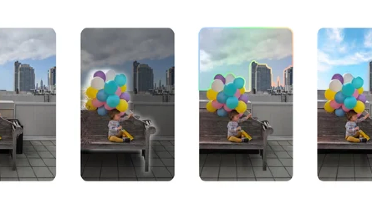
Magic Editor is an experimental editing experience that uses AI to help reimagine your photos — early access is planned for select Pixel phones later this year.Read More

 With advancements in AI, there are new ways to understand your route with Maps. Plus, new immersive tools for developers.Read More

 Starting today, you can sign up to try MusicLM, a new experimental AI tool that can turn your text descriptions into music.Read More
For decades, researchers worked together to assemble a complete copy of the molecular instructions for a human — a map of the human genome. The first draft was finished in 2000, but with several missing pieces. Even when a complete reference genome was achieved in 2022, their work was not finished. A single reference genome can’t incorporate known genetic variations, such as the variants for the gene determining whether a person has a blood type A, B, AB or O. Furthermore, the reference genome didn’t represent the vast diversity of human ancestries, making it less useful for detecting disease or finding cures for people from some backgrounds than others. For the past three years, we have been part of an international collaboration with 119 scientists across 60 institutions, called the Human Pangenome Research Consortium, to address these challenges by creating a new and more representative map of the human genome, a pangenome.
We are excited to share that today, in “A draft human pangenome reference”, published in Nature, this group is announcing the completion of the first human pangenome reference. The pangenome combines 47 individual genome reference sequences and better represents the genomic diversity of global populations. Building on Google’s deep learning technologies and past advances in genomics, we used tools based on convolutional neural networks (CNNs) and transformers to tackle the challenges of building accurate pangenome sequences and using them for genome analysis. These contributions helped the consortium build an information-rich resource for geneticists, researchers and clinicians around the world.
 |
In the typical analysis workflow for high-throughput DNA sequencing, a sequencing instrument reads millions of short pieces of an individual’s genome, and a program called a mapper or aligner then estimates where those pieces best fit relative to the single, linear human reference sequence. Next, variant caller software identifies the unique parts of the individual’s sequence relative to the reference.
But because humans carry a diverse set of sequences, sections that are present in an individual’s DNA but are not in the reference genome can’t be analyzed. One study of 910 African individuals found that a total of 300 million DNA base pairs — 10% of the roughly three billion base pair reference genome — are not present in the previous linear reference but occur in at least one of the 910 individuals.
To address this issue, the consortium used graph data structures, which are powerful for genomics because they can represent the sequences of many people simultaneously, which is needed to create a pangenome. Nodes in a graph genome contain the known set of sequences in a population, and paths through those nodes compactly describe the unique sequences of an individual’s DNA.
 |
| Schematic of a graph genome. Each color represents the sequence path of a different individual. Multiple paths passing through the same node indicate multiple individuals share that sequence, but some paths also show a single nucleotide variant (SNV), insertions, or deletions. Illustration credit Darryl Leja, National Human Genome Research Institute (NHGRI). |
 |
| Actual graph genome for the major histocompatibility complex (MHC) region of the genome. Genes in MHC regions are essential to immune function and are associated with a person’s resistance and susceptibility to infectious disease and autoimmune disorders (e.g., ankylosing spondylitis and lupus). The graph shows the linear human genome reference (green) and different individual person’s sequence (gray). |
Using graphs creates numerous challenges. They require reference sequences to be highly accurate and the development of new methods that can use their data structure as an input. However, new sequencing technologies (such as consensus sequencing and phased assembly methods) have driven exciting progress towards solving these problems.
Long-read sequencing technology, which reads larger pieces of the genome (10,000 to millions of DNA characters long) at a time, are essential to the creation of high quality reference sequences because larger pieces can be stitched together into assembled genomes more easily than the short pieces read out by earlier technologies. Short read sequencing reads pieces of the genome that are only 100 to 300 DNA characters long, but has been the highly scalable basis for high-throughput sequencing methods developed in the 2000s. Though long-read sequencing is newer and has advantages for reference genome creation, many informatics methods for short reads hadn’t been developed for long read technologies.
Google initially developed DeepVariant, an open-source CNN variant caller framework that analyzes the short-read sequencing evidence of local regions of the genome. However, we were able to re-train DeepVariant to yield accurate analysis of Pacific Bioscience’s long-read data.
 |
| Training and evaluation schematic for DeepVariant. |
We next teamed up with researchers at the University of California, Santa Cruz (UCSC) Genomics Institute to participate in a United States Food and Drug Administration competition for another long-read sequencing technology from Oxford Nanopore. Together, we won the award for highest accuracy in the nanopore category, with a single nucleotide variants (SNVs) accuracy that matched short-read sequencing. This work has been used to detect and treat genetic diseases in critically ill newborns. The use of DeepVariant on long-read technologies provided the foundation for the consortium’s use of DeepVariant for error correction of pangenomes.
DeepVariant’s ability to use multiple long-read sequencing modalities proved useful for error correction in the Telomere-to-Telomere (T2T) Consortium’s effort that generated the first complete assembly of a human genome. Completing this first genome set the stage to build the multiple reference genomes required for pangenomes, and T2T was already working closely with the Human Pangenome Project (with many shared members) to scale those practices.
With a set of high-quality human reference genomes on the horizon, developing methods that could use those assemblies grew in importance. We worked to adapt DeepVariant to use the pangenome developed by the consortium. In partnership with UCSC, we built an end-to-end analysis workflow for graph-based variant detection, and demonstrated improved accuracy across several thousand samples. The use of the pangenome allows many previously missed variants to be correctly identified.
 |
| Visualization of variant calls in the KCNE1 gene (a gene with variants associated with cardiac arrhythmias and sudden death) using a pangenome reference versus the prior linear reference. Each dot represents a variant call that is either correct (blue dot), incorrect (green dot) — when a variant is identified but is not really there —or a missed variant call (red dot). The top box shows variant calls made by DeepVariant using the pangenome reference while the bottom shows variant calls made by using the linear reference. Figure adapted from A Draft Human Pangenome Reference. |
Just as new sequencing technologies enabled new pangenome approaches, new informatics technologies enabled improvements for sequencing methods. Google adapted transformer architectures from analysis of human language to genome sequences to develop DeepConsensus. A key enabler for this was the development of a differentiable loss function that could handle the insertions and deletions common in sequencing data. This enabled us to have high accuracy without needing a decoder, allowing the speed required to keep up with terabytes of sequencer output.
 |
| Transformer architecture for DeepConsensus. DeepConsensus takes as input the repeated sequence of the DNA molecule, measured from fluorescent light detected by the addition of each base. DeepConsensus also uses as input the more detailed information about the sequencing process, including the duration of the light pulse (referred to here as pulse width or PW), the time between pulses (IP) the signal-to-noise ratio (SN) and which side of the double helix is being measured (strand). |
 |
| Effect of alignment loss function in training evaluation of model output. Better accounting of insertions and deletions by a differentiable alignment function enables the model training process to better estimate errors. |
DeepConsensus improves the yield and accuracy of instrument data. Because PacBio sequencing provides the primary sequence information for the 47 genome assemblies, we could apply DeepConsensus to improve those assemblies. With application of DeepConsensus, consortium members built a genome assembler that was able to reach 99.9997% assembly base-level accuracies.
We developed multiple new approaches to improve genetic sequencing methods, which we then used to construct pangenome references that enable more robust genome analysis.
But this is just the beginning of the story. In the next stage, a larger, worldwide group of scientists and clinicians will use this pangenome reference to study genetic diseases and make new drugs. And future pangenomes will represent even more individuals, realizing a vision summarized this way in a recent Nature story: “Every base, everywhere, all at once.” Read our post on the Keyword Blog to learn more about the human pangenome reference announcement.
Many people were involved in creating the pangenome reference, including 119 authors across 60 organizations, with the Human Pangenome Reference Consortium. This blog post highlights Google’s contributions to the broader work. We thank the research groups at UCSC Genomics Institute (GI) under Professors Benedict Paten and Karen Miga, genome polishing efforts of Arang Rhie at National Institute of Health (NIH), Genome Assembly and Polishing of Adam Phillipy’s group, and the standards group at National Institute of Standards and Technology (NIST) of Justin Zook. We thank Google contributors: Pi-Chuan Chang, Maria Nattestad, Daniel Cook, Alexey Kolesnikov, Anastaysia Belyaeva, and Gunjan Baid. We thank Lizzie Dorfman, Elise Kleeman, Erika Hayden, Cory McLean, Shravya Shetty, Greg Corrado, Katherine Chou, and Yossi Matias for their support, coordination, and leadership. Last but not least, thanks to the research participants that provided their DNA to help build the pangenome resource.
 These startups are using AI to decarbonize buildings, create sustainable agriculture, protect biodiversity, and remove carbon from the atmosphere.Read More

Vision-language foundational models are built on the premise of a single pre-training followed by subsequent adaptation to multiple downstream tasks. Two main and disjoint training scenarios are popular: a CLIP-style contrastive learning and next-token prediction. Contrastive learning trains the model to predict if image-text pairs correctly match, effectively building visual and text representations for the corresponding image and text inputs, whereas next-token prediction predicts the most likely next text token in a sequence, thus learning to generate text, according to the required task. Contrastive learning enables image-text and text-image retrieval tasks, such as finding the image that best matches a certain description, and next-token learning enables text-generative tasks, such as Image Captioning and Visual Question Answering (VQA). While both approaches have demonstrated powerful results, when a model is pre-trained contrastively, it typically does not fare well on text-generative tasks and vice-versa. Furthermore, adaptation to other tasks is often done with complex or inefficient methods. For example, in order to extend a vision-language model to videos, some models need to do inference for each video frame separately. This limits the size of the videos that can be processed to only a few frames and does not fully take advantage of motion information available across frames.
Motivated by this, we present “A Simple Architecture for Joint Learning for MultiModal Tasks”, called MaMMUT, which is able to train jointly for these competing objectives and which provides a foundation for many vision-language tasks either directly or via simple adaptation. MaMMUT is a compact, 2B-parameter multimodal model that trains across contrastive, text generative, and localization-aware objectives. It consists of a single image encoder and a text decoder, which allows for a direct reuse of both components. Furthermore, a straightforward adaptation to video-text tasks requires only using the image encoder once and can handle many more frames than prior work. In line with recent language models (e.g., PaLM, GLaM, GPT3), our architecture uses a decoder-only text model and can be thought of as a simple extension of language models. While modest in size, our model outperforms the state of the art or achieves competitive performance on image-text and text-image retrieval, video question answering (VideoQA), video captioning, open-vocabulary detection, and VQA.
 |
 |
 |
| The MaMMUT model enables a wide range of tasks such as image-text/text-image retrieval (top left and top right), VQA (middle left), open-vocabulary detection (middle right), and VideoQA (bottom). |
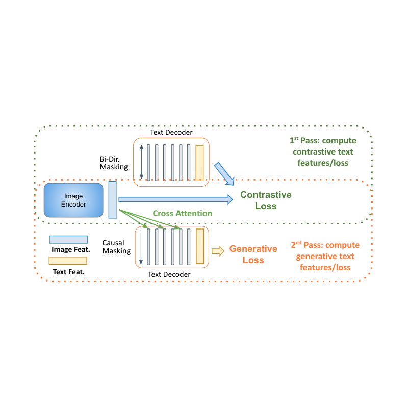
One surprising finding is that a single language-decoder is sufficient for all these tasks, which obviates the need for both complex constructs and training procedures presented before. For example, our model (presented to the left in the figure below) consists of a single visual encoder and single text-decoder, connected via cross attention, and trains simultaneously on both contrastive and text-generative types of losses. Comparatively, prior work is either not able to handle image-text retrieval tasks, or applies only some losses to only some parts of the model. To enable multimodal tasks and fully take advantage of the decoder-only model, we need to jointly train both contrastive losses and text-generative captioning-like losses.
 |
| MaMMUT architecture (left) is a simple construct consisting of a single vision encoder and a single text decoder. Compared to other popular vision-language models — e.g., PaLI (middle) and ALBEF, CoCa (right) — it trains jointly and efficiently for multiple vision-language tasks, with both contrastive and text-generative losses, fully sharing the weights between the tasks. |
Decoder-only models for language learning show clear advantages in performance with smaller model size (almost half the parameters). The main challenge for applying them to multimodal settings is to unify the contrastive learning (which uses unconditional sequence-level representation) with captioning (which optimizes the likelihood of a token conditioned on the previous tokens). We propose a two-pass approach to jointly learn these two conflicting types of text representations within the decoder. During the first pass, we utilize cross attention and causal masking to learn the caption generation task — the text features can attend to the image features and predict the tokens in sequence. On the second pass, we disable the cross-attention and causal masking to learn the contrastive task. The text features will not see the image features but can attend bidirectionally to all text tokens at once to produce the final text-based representation. Completing this two-pass approach within the same decoder allows for accommodating both types of tasks that were previously hard to reconcile. While simple, we show that this model architecture is able to provide a foundation for multiple multimodal tasks.
 |
| MaMMUT decoder-only two-pass learning enables both contrastive and generative learning paths by the same model. |
Another advantage of our architecture is that, since it is trained for these disjoint tasks, it can be seamlessly applied to multiple applications such as image-text and text-image retrieval, VQA, and captioning.
Moreover, MaMMUT easily adapts to video-language tasks. Previous approaches used a vision encoder to process each frame individually, which required applying it multiple times. This is slow and restricts the number of frames the model can handle, typically to only 6–8. With MaMMUT, we use sparse video tubes for lightweight adaptation directly via the spatio-temporal information from the video. Furthermore, adapting the model to Open-Vocabulary Detection is done by simply training to detect bounding-boxes via an object-detection head.
 |
| Adaptation of the MaMMUT architecture to video tasks (left) is simple and fully reuses the model. This is done by generating a video “tubes” feature representation, similar to image patches, that are projected to lower dimensional tokens and run through the vision encoder. Unlike prior approaches (right) that need to run multiple individual images through the vision encoder, we use it only once. |
Our model achieves excellent zero-shot results on image-text and text-image retrieval without any adaptation, outperforming all previous state-of-the-art models. The results on VQA are competitive with state-of-the-art results, which are achieved by much larger models. The PaLI model (17B parameters) and the Flamingo model (80B) have the best performance on the VQA2.0 dataset, but MaMMUT (2B) has the same accuracy as the 15B PaLI.
 |
 |
| MaMMUT outperforms the state of the art (SOTA) on Zero-Shot Image-Text (I2T) and Text-Image (T2I) retrieval on both MS-COCO (top) and Flickr (bottom) benchmarks. |
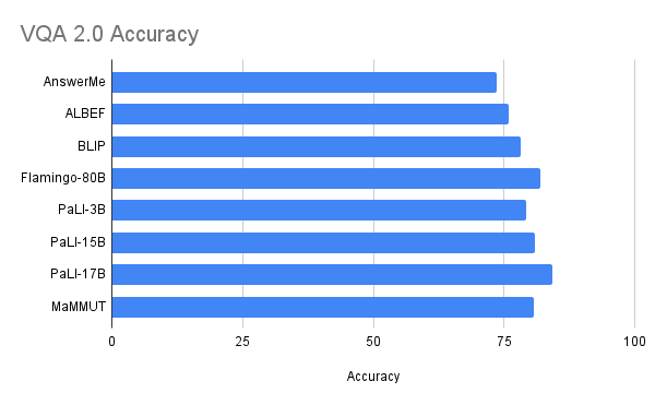 |
| Performance on the VQA2.0 dataset is competitive but does not outperform large models such as Flamingo-80B and PalI-17B. Performance is evaluated in the more challenging open-ended text generation setting. |
MaMMUT also outperforms the state-of-the-art on VideoQA, as shown below on the MSRVTT-QA and MSVD-QA datasets. Note that we outperform much bigger models such as Flamingo, which is specifically designed for image+video pre-training and is pre-trained with both image-text and video-text data.
 |
 |
| MaMMUT outperforms the SOTA models on VideoQA tasks (MSRVTT-QA dataset, top, MSVD-QA dataset, bottom), outperforming much larger models, e.g., the 5B GIT2 or Flamingo, which uses 80B parameters and is pre-trained for both image-language and vision-language tasks. |
Our results outperform the state-of-the-art on open-vocabulary detection fine-tuning as is also shown below.
 |
| MAMMUT open-vocabulary detection results on the LVIS dataset compared to state-of-the-art methods. We report the average precisions for rare classes (APr) as is previously adopted in the literature. |
We show that joint training of both contrastive and text-generative objectives is not an easy task, and in our ablations we find that these tasks are served better by different design choices. We see that fewer cross-attention connections are better for retrieval tasks, but more are preferred by VQA tasks. Yet, while this shows that our model’s design choices might be suboptimal for individual tasks, our model is more effective than more complex, or larger, models.
 |
 |
| Ablation studies showing that fewer cross-attention connections (1-2) are better for retrieval tasks (top), whereas more connections favor text-generative tasks such as VQA (bottom). |
We presented MaMMUT, a simple and compact vision-encoder language-decoder model that jointly trains a number of conflicting objectives to reconcile contrastive-like and text-generative tasks. Our model also serves as a foundation for many more vision-language tasks, achieving state-of-the-art or competitive performance on image-text and text-image retrieval, videoQA, video captioning, open-vocabulary detection and VQA. We hope it can be further used for more multimodal applications.
The work described is co-authored by: Weicheng Kuo, AJ Piergiovanni, Dahun Kim, Xiyang Luo, Ben Caine, Wei Li, Abhijit Ogale, Luowei Zhou, Andrew Dai, Zhifeng Chen, Claire Cui, and Anelia Angelova. We would like to thank Mojtaba Seyedhosseini, Vijay Vasudevan, Priya Goyal, Jiahui Yu, Zirui Wang, Yonghui Wu, Runze Li, Jie Mei, Radu Soricut, Qingqing Huang, Andy Ly, Nan Du, Yuxin Wu, Tom Duerig, Paul Natsev, Zoubin Ghahramani for their help and support.

Teaching mobile robots to navigate in complex outdoor environments is critical to real-world applications, such as delivery or search and rescue. However, this is also a challenging problem as the robot needs to perceive its surroundings, and then explore to identify feasible paths towards the goal. Another common challenge is that the robot needs to overcome uneven terrains, such as stairs, curbs, or rockbed on a trail, while avoiding obstacles and pedestrians. In our prior work, we investigated the second challenge by teaching a quadruped robot to tackle challenging uneven obstacles and various outdoor terrains.
In “IndoorSim-to-OutdoorReal: Learning to Navigate Outdoors without any Outdoor Experience”, we present our recent work to tackle the robotic challenge of reasoning about the perceived surroundings to identify a viable navigation path in outdoor environments. We introduce a learning-based indoor-to-outdoor transfer algorithm that uses deep reinforcement learning to train a navigation policy in simulated indoor environments, and successfully transfers that same policy to real outdoor environments. We also introduce Context-Maps (maps with environment observations created by a user), which are applied to our algorithm to enable efficient long-range navigation. We demonstrate that with this policy, robots can successfully navigate hundreds of meters in novel outdoor environments, around previously unseen outdoor obstacles (trees, bushes, buildings, pedestrians, etc.), and in different weather conditions (sunny, overcast, sunset).
User inputs can tell a robot where to go with commands like “go to the Android statue”, pictures showing a target location, or by simply picking a point on a map. In this work, we specify the navigation goal (a selected point on a map) as a relative coordinate to the robot’s current position (i.e., “go to ∆x, ∆y”), this is also known as the PointGoal Visual Navigation (PointNav) task. PointNav is a general formulation for navigation tasks and is one of the standard choices for indoor navigation tasks. However, due to the diverse visuals, uneven terrains and long distance goals in outdoor environments, training PointNav policies for outdoor environments is a challenging task.
Recent successes in training wheeled and legged robotic agents to navigate in indoor environments were enabled by the development of fast, scalable simulators and the availability of large-scale datasets of photorealistic 3D scans of indoor environments. To leverage these successes, we develop an indoor-to-outdoor transfer technique that enables our robots to learn from simulated indoor environments and to be deployed in real outdoor environments.
To overcome the differences between simulated indoor environments and real outdoor environments, we apply kinematic control and image augmentation techniques in our learning system. When using kinematic control, we assume the existence of a reliable low-level locomotion controller that can control the robot to precisely reach a new location. This assumption allows us to directly move the robot to the target location during simulation training through a forward Euler integration and relieves us from having to explicitly model the underlying robot dynamics in simulation, which drastically improves the throughput of simulation data generation. Prior work has shown that kinematic control can lead to better sim-to-real transfer compared to a dynamic control approach, where full robot dynamics are modeled and a low-level locomotion controller is required for moving the robot.
| Left Kinematic control; Right: Dynamic control |
We created an outdoor maze-like environment using objects found indoors for initial experiments, where we used Boston Dynamics’ Spot robot for test navigation. We found that the robot could navigate around novel obstacles in the new outdoor environment.
| The Spot robot successfully navigates around obstacles found in indoor environments, with a policy trained entirely in simulation. |
However, when faced with unfamiliar outdoor obstacles not seen during training, such as a large slope, the robot was unable to navigate the slope.
| The robot is unable to navigate up slopes, as slopes are rare in indoor environments and the robot was not trained to tackle it. |
To enable the robot to walk up and down slopes, we apply an image augmentation technique during the simulation training. Specifically, we randomly tilt the simulated camera on the robot during training. It can be pointed up or down within 30 degrees. This augmentation effectively makes the robot perceive slopes even though the floor is level. Training on these perceived slopes enables the robot to navigate slopes in the real-world.
| By randomly tilting the camera angle during training in simulation, the robot is now able to walk up and down slopes. |
Since the robots were only trained in simulated indoor environments, in which they typically need to walk to a goal just a few meters away, we find that the learned network failed to process longer-range inputs — e.g., the policy failed to walk forward for 100 meters in an empty space. To enable the policy network to handle long-range inputs that are common for outdoor navigation, we normalize the goal vector by using the log of the goal distance.
Putting everything together, the robot can navigate outdoors towards the goal, while walking on uneven terrain, and avoiding trees, pedestrians and other outdoor obstacles. However, there is still one key component missing: the robot’s ability to plan an efficient long-range path. At this scale of navigation, taking a wrong turn and backtracking can be costly. For example, we find that the local exploration strategy learned by standard PointNav policies are insufficient in finding a long-range goal and usually leads to a dead end (shown below). This is because the robot is navigating without context of its environment, and the optimal path may not be visible to the robot from the start.
| Navigation policies without context of the environment do not handle complex long-range navigation goals. |
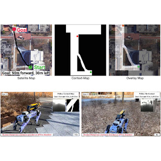
To enable the robot to take the context into consideration and purposefully plan an efficient path, we provide a Context-Map (a binary image that represents a top-down occupancy map of the region that the robot is within) as additional observations for the robot. An example Context-Map is given below, where the black region denotes areas occupied by obstacles and white region is walkable by the robot. The green and red circle denotes the start and goal location of the navigation task. Through the Context-Map, we can provide hints to the robot (e.g., the narrow opening in the route below) to help it plan an efficient navigation route. In our experiments, we create the Context-Map for each route guided by Google Maps satellite images. We denote this variant of PointNav with environmental context, as Context-Guided PointNav.
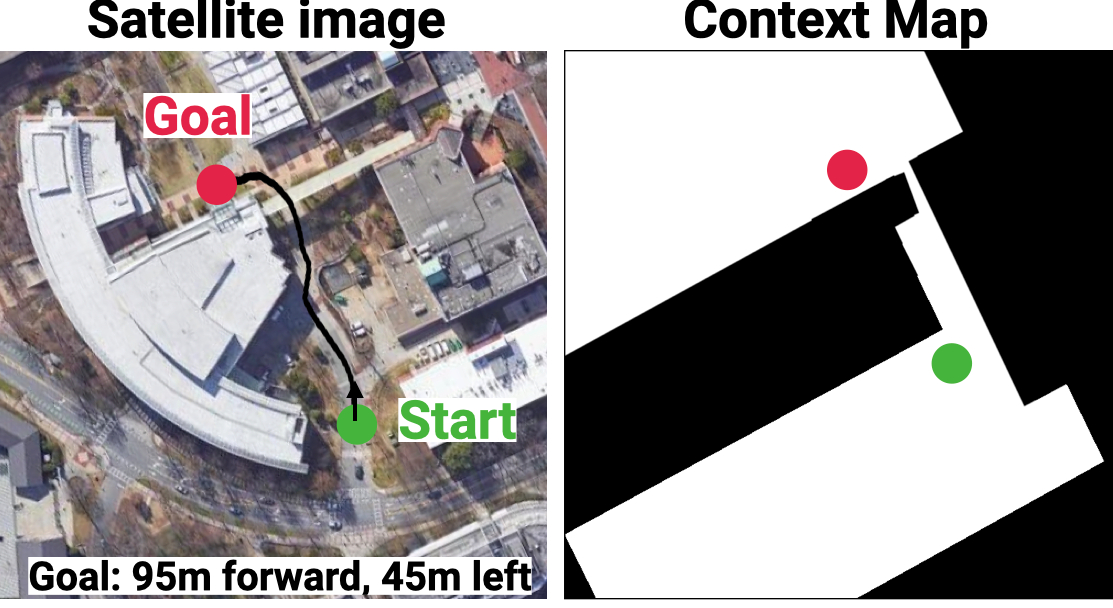 |
| Example of the Context-Map (right) for a navigation task (left). |
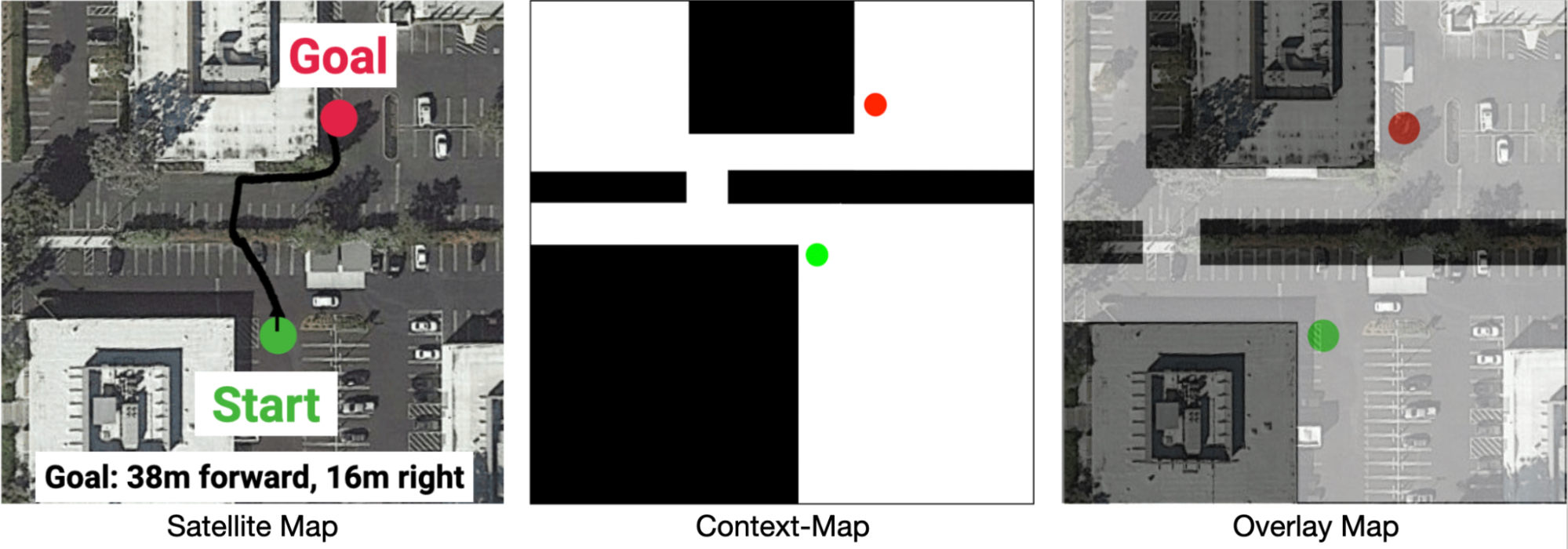
It is important to note that the Context-Map does not need to be accurate because it only serves as a rough outline for planning. During navigation, the robot still needs to rely on its onboard cameras to identify and adapt its path to pedestrians, which are absent on the map. In our experiments, a human operator quickly sketches the Context-Map from the satellite image, masking out the regions to be avoided. This Context-Map, together with other onboard sensory inputs, including depth images and relative position to the goal, are fed into a neural network with attention models (i.e., transformers), which are trained using DD-PPO, a distributed implementation of proximal policy optimization, in large-scale simulations.
 |
| The Context-Guided PointNav architecture consists of a 3-layer convolutional neural network (CNN) to process depth images from the robot’s camera, and a multilayer perceptron (MLP) to process the goal vector. The features are passed into a gated recurrent unit (GRU). We use an additional CNN encoder to process the context-map (top-down map). We compute the scaled dot product attention between the map and the depth image, and use a second GRU to process the attended features (Context Attn., Depth Attn.). The output of the policy are linear and angular velocities for the Spot robot to follow. |
We evaluate our system across three long-range outdoor navigation tasks. The provided Context-Maps are rough, incomplete environment outlines that omit obstacles, such as cars, trees, or chairs.
With the proposed algorithm, our robot can successfully reach the distant goal location 100% of the time, without a single collision or human intervention. The robot was able to navigate around pedestrians and real-world clutter that are not present on the context-map, and navigate on various terrain including dirt slopes and grass.
 |
 |
 |
This work opens up robotic navigation research to the less explored domain of diverse outdoor environments. Our indoor-to-outdoor transfer algorithm uses zero real-world experience and does not require the simulator to model predominantly-outdoor phenomena (terrain, ditches, sidewalks, cars, etc). The success in the approach comes from a combination of a robust locomotion control, low sim-to-real gap in depth and map sensors, and large-scale training in simulation. We demonstrate that providing robots with approximate, high-level maps can enable long-range navigation in novel outdoor environments. Our results provide compelling evidence for challenging the (admittedly reasonable) hypothesis that a new simulator must be designed for every new scenario we wish to study. For more information, please see our project page.
We would like to thank Sonia Chernova, Tingnan Zhang, April Zitkovich, Dhruv Batra, and Jie Tan for advising and contributing to the project. We would also like to thank Naoki Yokoyama, Nubby Lee, Diego Reyes, Ben Jyenis, and Gus Kouretas for help with the robot experiment setup.

 Checks takes the complexity out of compliance, using AI to help companies quickly discover, communicate and fix issues.Read More

 Four new online interactive artworks from Google Arts & Culture Lab artists in residenceRead More


The Eleventh International Conference on Learning Representations (ICLR 2023) is being held this week as a hybrid event in Kigali, Rwanda. We are proud to be a Diamond Sponsor of ICLR 2023, a premier conference on deep learning, where Google researchers contribute at all levels. This year we are presenting over 100 papers and are actively involved in organizing and hosting a number of different events, including workshops and interactive sessions.
If you’re registered for ICLR 2023, we hope you’ll visit the Google booth to learn more about the exciting work we’re doing across topics spanning representation and reinforcement learning, theory and optimization, social impact, safety and privacy, and applications from generative AI to speech and robotics. Continue below to find the many ways in which Google researchers are engaged at ICLR 2023, including workshops, papers, posters and talks (Google affiliations in bold).
Board Members include: Shakir Mohamed, Tara Sainath
Senior Program Chairs include: Been Kim
Workshop Chairs include: Aisha Walcott-Bryant, Rose Yu
Diversity, Equity & Inclusion Chairs include: Rosanne Liu
Emergence of Maps in the Memories of Blind Navigation Agents
Erik Wijmans, Manolis Savva, Irfan Essa, Stefan Lee, Ari S. Morcos, Dhruv Batra
DreamFusion: Text-to-3D Using 2D Diffusion
Ben Poole, Ajay Jain, Jonathan T. Barron, Ben Mildenhall
Learned Optimizers: Why They’re the Future, Why They’re Hard, and What They Can Do Now
Jascha Sohl-Dickstein
Kaggle@ICLR 2023: ML Solutions in Africa
Organizers include: Julia Elliott, Phil Culliton, Ray Harvey
Facilitators: Julia Elliot, Walter Reade
Reincarnating Reinforcement Learning (Reincarnating RL)
Organizers include: Rishabh Agarwal, Ted Xiao, Max Schwarzer
Speakers include: Sergey Levine
Panelists include: Marc G. Bellemare, Sergey Levine
Trustworthy and Reliable Large-Scale Machine Learning Models
Organizers include: Sanmi Koyejo
Speakers include: Nicholas Carlini
Physics for Machine Learning (Physics4ML)
Speakers include: Yasaman Bahri
AI for Agent-Based Modelling Community (AI4ABM)
Organizers include: Pablo Samuel Castro
Mathematical and Empirical Understanding of Foundation Models (ME-FoMo)
Organizers include: Mathilde Caron, Tengyu Ma, Hanie Sedghi
Speakers include: Yasaman Bahri, Yann Dauphin
Neurosymbolic Generative Models 2023 (NeSy-GeMs)
Organizers include: Kevin Ellis
Speakers include: Daniel Tarlow, Tuan Anh Le
What Do We Need for Successful Domain Generalization?
Panelists include: Boqing Gong
The 4th Workshop on Practical ML for Developing Countries: Learning Under Limited/Low Resource Settings
Keynote Speaker: Adji Bousso Dieng
Machine Learning for Remote Sensing
Speakers include: Abigail Annkah
Multimodal Representation Learning (MRL): Perks and Pitfalls
Organizers include: Petra Poklukar
Speakers include: Arsha Nagrani
Pitfalls of Limited Data and Computation for Trustworthy ML
Organizers include: Prateek Jain
Speakers include: Nicholas Carlini, Praneeth Netrapalli
Sparsity in Neural Networks: On Practical Limitations and Tradeoffs Between Sustainability and Efficiency
Organizers include: Trevor Gale, Utku Evci
Speakers include: Aakanksha Chowdhery, Jeff Dean
Time Series Representation Learning for Health
Speakers include: Katherine Heller
Deep Learning for Code (DL4C)
Organizers include: Gabriel Orlanski
Speakers include: Alex Polozov, Daniel Tarlow
Tiny Papers Showcase Day (a DEI initiative)
Organizers include: Rosanne Liu
Evolve Smoothly, Fit Consistently: Learning Smooth Latent Dynamics for Advection-Dominated Systems
Zhong Yi Wan, Leonardo Zepeda-Nunez, Anudhyan Boral, Fei Sha
Quantifying Memorization Across Neural Language Models
Nicholas Carlini, Daphne Ippolito, Matthew Jagielski, Katherine Lee, Florian Tramer, Chiyuan Zhang
Emergence of Maps in the Memories of Blind Navigation Agents (Outstanding Paper Award)
Erik Wijmans, Manolis Savva, Irfan Essa, Stefan Lee, Ari S. Morcos, Dhruv Batra
Offline Q-Learning on Diverse Multi-task Data Both Scales and Generalizes (see blog post)
Aviral Kumar, Rishabh Agarwal, Xingyang Geng, George Tucker, Sergey Levine
ReAct: Synergizing Reasoning and Acting in Language Models (see blog post)
Shunyu Yao*, Jeffrey Zhao, Dian Yu, Nan Du, Izhak Shafran, Karthik R. Narasimhan, Yuan Cao
Prompt-to-Prompt Image Editing with Cross-Attention Control
Amir Hertz, Ron Mokady, Jay Tenenbaum, Kfir Aberman, Yael Pritch, Daniel Cohen-Or
DreamFusion: Text-to-3D Using 2D Diffusion (Outstanding Paper Award)
Ben Poole, Ajay Jain, Jonathan T. Barron, Ben Mildenhall
A System for Morphology-Task Generalization via Unified Representation and Behavior Distillation
Hiroki Furuta, Yusuke Iwasawa, Yutaka Matsuo, Shixiang Shane Gu
Sample-Efficient Reinforcement Learning by Breaking the Replay Ratio Barrier
Pierluca D’Oro, Max Schwarzer, Evgenii Nikishin, Pierre-Luc Bacon, Marc G Bellemare, Aaron Courville
Dichotomy of Control: Separating What You Can Control from What You Cannot
Sherry Yang, Dale Schuurmans, Pieter Abbeel, Ofir Nachum
Fast and Precise: Adjusting Planning Horizon with Adaptive Subgoal Search
Michał Zawalski, Michał Tyrolski, Konrad Czechowski, Tomasz Odrzygóźdź, Damian Stachura, Piotr Piekos, Yuhuai Wu, Łukasz Kucinski, Piotr Miłos
The Trade-Off Between Universality and Label Efficiency of Representations from Contrastive Learning
Zhenmei Shi, Jiefeng Chen, Kunyang Li, Jayaram Raghuram, Xi Wu, Yingyu Liang, Somesh Jha
Sparsity-Constrained Optimal Transport
Tianlin Liu*, Joan Puigcerver, Mathieu Blondel
Unmasking the Lottery Ticket Hypothesis: What’s Encoded in a Winning Ticket’s Mask?
Mansheej Paul, Feng Chen, Brett W. Larsen, Jonathan Frankle, Surya Ganguli, Gintare Karolina Dziugaite
Extreme Q-Learning: MaxEnt RL without Entropy
Divyansh Garg, Joey Hejna, Matthieu Geist, Stefano Ermon
Draft, Sketch, and Prove: Guiding Formal Theorem Provers with Informal Proofs
Albert Qiaochu Jiang, Sean Welleck, Jin Peng Zhou, Timothee Lacroix, Jiacheng Liu, Wenda Li, Mateja Jamnik, Guillaume Lample, Yuhuai Wu
SimPer: Simple Self-Supervised Learning of Periodic Targets
Yuzhe Yang, Xin Liu, Jiang Wu, Silviu Borac, Dina Katabi, Ming-Zher Poh, Daniel McDuff
Socratic Models: Composing Zero-Shot Multimodal Reasoning with Language
Andy Zeng, Maria Attarian, Brian Ichter, Krzysztof Marcin Choromanski, Adrian Wong, Stefan Welker, Federico Tombari, Aveek Purohit, Michael S. Ryoo, Vikas Sindhwani, Johnny Lee, Vincent Vanhoucke, Pete Florence
What Learning Algorithm Is In-Context Learning? Investigations with Linear Models
Ekin Akyurek*, Dale Schuurmans, Jacob Andreas, Tengyu Ma*, Denny Zhou
Preference Transformer: Modeling Human Preferences Using Transformers for RL
Changyeon Kim, Jongjin Park, Jinwoo Shin, Honglak Lee, Pieter Abbeel, Kimin Lee
Iterative Patch Selection for High-Resolution Image Recognition
Benjamin Bergner, Christoph Lippert, Aravindh Mahendran
Open-Vocabulary Object Detection upon Frozen Vision and Language Models
Weicheng Kuo, Yin Cui, Xiuye Gu, AJ Piergiovanni, Anelia Angelova
(Certified!!) Adversarial Robustness for Free!
Nicholas Carlini, Florian Tramér, Krishnamurthy (Dj) Dvijotham, Leslie Rice, Mingjie Sun, J. Zico Kolter
REPAIR: REnormalizing Permuted Activations for Interpolation Repair
Keller Jordan, Hanie Sedghi, Olga Saukh, Rahim Entezari, Behnam Neyshabur
Discrete Predictor-Corrector Diffusion Models for Image Synthesis
José Lezama, Tim Salimans, Lu Jiang, Huiwen Chang, Jonathan Ho, Irfan Essa
Feature Reconstruction From Outputs Can Mitigate Simplicity Bias in Neural Networks
Sravanti Addepalli, Anshul Nasery, Praneeth Netrapalli, Venkatesh Babu R., Prateek Jain
An Exact Poly-time Membership-Queries Algorithm for Extracting a Three-Layer ReLU Network
Amit Daniely, Elad Granot
Language Models Are Multilingual Chain-of-Thought Reasoners
Freda Shi, Mirac Suzgun, Markus Freitag, Xuezhi Wang, Suraj Srivats, Soroush Vosoughi, Hyung Won Chung, Yi Tay, Sebastian Ruder, Denny Zhou, Dipanjan Das, Jason Wei
Scaling Forward Gradient with Local Losses
Mengye Ren*, Simon Kornblith, Renjie Liao, Geoffrey Hinton
Treeformer: Dense Gradient Trees for Efficient Attention Computation
Lovish Madaan, Srinadh Bhojanapalli, Himanshu Jain, Prateek Jain
LilNetX: Lightweight Networks with EXtreme Model Compression and Structured Sparsification
Sharath Girish, Kamal Gupta, Saurabh Singh, Abhinav Shrivastava
DiffusER: Diffusion via Edit-Based Reconstruction
Machel Reid, Vincent J. Hellendoorn, Graham Neubig
Leveraging Unlabeled Data to Track Memorization
Mahsa Forouzesh, Hanie Sedghi, Patrick Thiran
A Mixture-of-Expert Approach to RL-Based Dialogue Management
Yinlam Chow, Aza Tulepbergenov, Ofir Nachum, Dhawal Gupta, Moonkyung Ryu, Mohammad Ghavamzadeh, Craig Boutilier
Easy Differentially Private Linear Regression
Kareem Amin, Matthew Joseph, Monica Ribero, Sergei Vassilvitskii
KwikBucks: Correlation Clustering with Cheap-Weak and Expensive-Strong Signals
Sandeep Silwal*, Sara Ahmadian, Andrew Nystrom, Andrew McCallum, Deepak Ramachandran, Mehran Kazemi
Massively Scaling Heteroscedastic Classifiers
Mark Collier, Rodolphe Jenatton, Basil Mustafa, Neil Houlsby, Jesse Berent, Effrosyni Kokiopoulou
The Lazy Neuron Phenomenon: On Emergence of Activation Sparsity in Transformers
Zonglin Li, Chong You, Srinadh Bhojanapalli, Daliang Li, Ankit Singh Rawat, Sashank J. Reddi, Ke Ye, Felix Chern, Felix Yu, Ruiqi Guo, Sanjiv Kumar
Compositional Semantic Parsing with Large Language Models
Andrew Drozdov, Nathanael Scharli, Ekin Akyurek, Nathan Scales, Xinying Song, Xinyun Chen, Olivier Bousquet, Denny Zhou
Extremely Simple Activation Shaping for Out-of-Distribution Detection
Andrija Djurisic, Nebojsa Bozanic, Arjun Ashok, Rosanne Liu
Long Range Language Modeling via Gated State Spaces
Harsh Mehta, Ankit Gupta, Ashok Cutkosky, Behnam Neyshabur
Investigating Multi-task Pretraining and Generalization in Reinforcement Learning
Adrien Ali Taiga, Rishabh Agarwal, Jesse Farebrother, Aaron Courville, Marc G. Bellemare
Learning Low Dimensional State Spaces with Overparameterized Recurrent Neural Nets
Edo Cohen-Karlik, Itamar Menuhin-Gruman, Raja Giryes, Nadav Cohen, Amir Globerson
Weighted Ensemble Self-Supervised Learning
Yangjun Ruan*, Saurabh Singh, Warren Morningstar, Alexander A. Alemi, Sergey Ioffe, Ian Fischer, Joshua V. Dillon
Calibrating Sequence Likelihood Improves Conditional Language Generation
Yao Zhao, Misha Khalman, Rishabh Joshi, Shashi Narayan, Mohammad Saleh, Peter J. Liu
SMART: Sentences as Basic Units for Text Evaluation
Reinald Kim Amplayo, Peter J. Liu, Yao Zhao, Shashi Narayan
Leveraging Importance Weights in Subset Selection
Gui Citovsky, Giulia DeSalvo, Sanjiv Kumar, Srikumar Ramalingam, Afshin Rostamizadeh, Yunjuan Wang*
Proto-Value Networks: Scaling Representation Learning with Auxiliary Tasks
Jesse Farebrother, Joshua Greaves, Rishabh Agarwal, Charline Le Lan, Ross Goroshin, Pablo Samuel Castro, Marc G. Bellemare
An Extensible Multi-modal Multi-task Object Dataset with Materials
Trevor Standley, Ruohan Gao, Dawn Chen, Jiajun Wu, Silvio Savarese
Measuring Forgetting of Memorized Training Examples
Matthew Jagielski, Om Thakkar, Florian Tramér, Daphne Ippolito, Katherine Lee, Nicholas Carlini, Eric Wallace, Shuang Song, Abhradeep Thakurta, Nicolas Papernot, Chiyuan Zhang
Bidirectional Language Models Are Also Few-Shot Learners
Ajay Patel, Bryan Li, Mohammad Sadegh Rasooli, Noah Constant, Colin Raffel, Chris Callison-Burch
Is Attention All That NeRF Needs?
Mukund Varma T., Peihao Wang, Xuxi Chen, Tianlong Chen, Subhashini Venugopalan, Zhangyang Wang
Automating Nearest Neighbor Search Configuration with Constrained Optimization
Philip Sun, Ruiqi Guo, Sanjiv Kumar
Static Prediction of Runtime Errors by Learning to Execute Programs with External Resource Descriptions
David Bieber, Rishab Goel, Daniel Zheng, Hugo Larochelle, Daniel Tarlow
Composing Ensembles of Pre-trained Models via Iterative Consensus
Shuang Li, Yilun Du, Joshua B. Tenenbaum, Antonio Torralba, Igor Mordatch
Λ-DARTS: Mitigating Performance Collapse by Harmonizing Operation Selection Among Cells
Sajad Movahedi, Melika Adabinejad, Ayyoob Imani, Arezou Keshavarz, Mostafa Dehghani, Azadeh Shakery, Babak N. Araabi
Blurring Diffusion Models
Emiel Hoogeboom, Tim Salimans
Part-Based Models Improve Adversarial Robustness
Chawin Sitawarin, Kornrapat Pongmala, Yizheng Chen, Nicholas Carlini, David Wagner
Learning in Temporally Structured Environments
Matt Jones, Tyler R. Scott, Mengye Ren, Gamaleldin ElSayed, Katherine Hermann, David Mayo, Michael C. Mozer
SlotFormer: Unsupervised Visual Dynamics Simulation with Object-Centric Models
Ziyi Wu, Nikita Dvornik, Klaus Greff, Thomas Kipf, Animesh Garg
Robust Algorithms on Adaptive Inputs from Bounded Adversaries
Yeshwanth Cherapanamjeri, Sandeep Silwal, David P. Woodruff, Fred Zhang, Qiuyi (Richard) Zhang, Samson Zhou
Agnostic Learning of General ReLU Activation Using Gradient Descent
Pranjal Awasthi, Alex Tang, Aravindan Vijayaraghavan
Analog Bits: Generating Discrete Data Using Diffusion Models with Self-Conditioning
Ting Chen, Ruixiang Zhang, Geoffrey Hinton
Any-Scale Balanced Samplers for Discrete Space
Haoran Sun*, Bo Dai, Charles Sutton, Dale Schuurmans, Hanjun Dai
Augmentation with Projection: Towards an Effective and Efficient Data Augmentation Paradigm for Distillation
Ziqi Wang*, Yuexin Wu, Frederick Liu, Daogao Liu, Le Hou, Hongkun Yu, Jing Li, Heng Ji
Beyond Lipschitz: Sharp Generalization and Excess Risk Bounds for Full-Batch GD
Konstantinos E. Nikolakakis, Farzin Haddadpour, Amin Karbasi, Dionysios S. Kalogerias
Causal Estimation for Text Data with (Apparent) Overlap Violations
Lin Gui, Victor Veitch
Contrastive Learning Can Find an Optimal Basis for Approximately View-Invariant Functions
Daniel D. Johnson, Ayoub El Hanchi, Chris J. Maddison
Differentially Private Adaptive Optimization with Delayed Preconditioners
Tian Li, Manzil Zaheer, Ziyu Liu, Sashank Reddi, Brendan McMahan, Virginia Smith
Distributionally Robust Post-hoc Classifiers Under Prior Shifts
Jiaheng Wei*, Harikrishna Narasimhan, Ehsan Amid, Wen-Sheng Chu, Yang Liu, Abhishek Kumar
Human Alignment of Neural Network Representations
Lukas Muttenthaler, Jonas Dippel, Lorenz Linhardt, Robert A. Vandermeulen, Simon Kornblith
Implicit Bias in Leaky ReLU Networks Trained on High-Dimensional Data
Spencer Frei, Gal Vardi, Peter Bartlett, Nathan Srebro, Wei Hu
Koopman Neural Operator Forecaster for Time-Series with Temporal Distributional Shifts
Rui Wang*, Yihe Dong, Sercan Ö. Arik, Rose Yu
Latent Variable Representation for Reinforcement Learning
Tongzheng Ren, Chenjun Xiao, Tianjun Zhang, Na Li, Zhaoran Wang, Sujay Sanghavi, Dale Schuurmans, Bo Dai
Least-to-Most Prompting Enables Complex Reasoning in Large Language Models
Denny Zhou, Nathanael Scharli, Le Hou, Jason Wei, Nathan Scales, Xuezhi Wang, Dale Schuurmans, Claire Cui, Olivier Bousquet, Quoc Le, Ed Chi
Mind’s Eye: Grounded Language Model Reasoning Through Simulation
Ruibo Liu, Jason Wei, Shixiang Shane Gu, Te-Yen Wu, Soroush Vosoughi, Claire Cui, Denny Zhou, Andrew M. Dai
MOAT: Alternating Mobile Convolution and Attention Brings Strong Vision Models
Chenglin Yang*, Siyuan Qiao, Qihang Yu, Xiaoding Yuan, Yukun Zhu, Alan Yuille, Hartwig Adam, Liang-Chieh Chen
Novel View Synthesis with Diffusion Models
Daniel Watson, William Chan, Ricardo Martin-Brualla, Jonathan Ho, Andrea Tagliasacchi, Mohammad Norouzi
On Accelerated Perceptrons and Beyond
Guanghui Wang, Rafael Hanashiro, Etash Guha, Jacob Abernethy
On Compositional Uncertainty Quantification for Seq2seq Graph Parsing
Zi Lin*, Du Phan, Panupong Pasupat, Jeremiah Liu, Jingbo Shang
On the Robustness of Safe Reinforcement Learning Under Observational Perturbations
Zuxin Liu, Zijian Guo, Zhepeng Cen, Huan Zhang, Jie Tan, Bo Li, Ding Zhao
Online Low Rank Matrix Completion
Prateek Jain, Soumyabrata Pal
Out-of-Distribution Detection and Selective Generation for Conditional Language Models
Jie Ren, Jiaming Luo, Yao Zhao, Kundan Krishna*, Mohammad Saleh, Balaji Lakshminarayanan, Peter J. Liu
PaLI: A Jointly-Scaled Multilingual Language-Image Model
Xi Chen, Xiao Wang, Soravit Changpinyo, AJ Piergiovanni, Piotr Padlewski, Daniel Salz, Sebastian Goodman, Adam Grycner, Basil Mustafa, Lucas Beyer, Alexander Kolesnikov, Joan Puigcerver, Nan Ding, Keran Rong, Hassan Akbari, Gaurav Mishra, Linting Xue, Ashish V. Thapliyal, James Bradbury, Weicheng Kuo, Mojtaba Seyedhosseini, Chao Jia, Burcu Karagol Ayan, Carlos Riquelme Ruiz, Andreas Peter Steiner, Anelia Angelova, Xiaohua Zhai, Neil Houlsby, Radu Soricut
Phenaki: Variable Length Video Generation from Open Domain Textual Descriptions
Ruben Villegas, Mohammad Babaeizadeh, Pieter-Jan Kindermans, Hernan Moraldo, Han Zhang, Mohammad Taghi Saffar, Santiago Castro*, Julius Kunze*, Dumitru Erhan
Promptagator: Few-Shot Dense Retrieval from 8 Examples
Zhuyun Dai, Vincent Y. Zhao, Ji Ma, Yi Luan, Jianmo Ni, Jing Lu, Anton Bakalov, Kelvin Guu, Keith B. Hall, Ming-Wei Chang
Pushing the Accuracy-Group Robustness Frontier with Introspective Self-Play
Jeremiah Zhe Liu, Krishnamurthy Dj Dvijotham, Jihyeon Lee, Quan Yuan, Balaji Lakshminarayanan, Deepak Ramachandran
Re-Imagen: Retrieval-Augmented Text-to-Image Generator
Wenhu Chen, Hexiang Hu, Chitwan Saharia, William W. Cohen
Recitation-Augmented Language Models
Zhiqing Sun, Xuezhi Wang, Yi Tay, Yiming Yang, Denny Zhou
Regression with Label Differential Privacy
Badih Ghazi, Pritish Kamath, Ravi Kumar, Ethan Leeman, Pasin Manurangsi, Avinash Varadarajan, Chiyuan Zhang
Revisiting the Entropy Semiring for Neural Speech Recognition
Oscar Chang, Dongseong Hwang, Olivier Siohan
Robust Active Distillation
Cenk Baykal, Khoa Trinh, Fotis Iliopoulos, Gaurav Menghani, Erik Vee
Score-Based Continuous-Time Discrete Diffusion Models
Haoran Sun*, Lijun Yu, Bo Dai, Dale Schuurmans, Hanjun Dai
Self-Consistency Improves Chain of Thought Reasoning in Language Models
Xuezhi Wang, Jason Wei, Dale Schuurmans, Quoc Le, Ed H. Chi, Sharan Narang, Aakanksha Chowdhery, Denny Zhou
Self-Supervision Through Random Segments with Autoregressive Coding (RandSAC)
Tianyu Hua, Yonglong Tian, Sucheng Ren, Michalis Raptis, Hang Zhao, Leonid Sigal
Serving Graph Compression for Graph Neural Networks
Si Si, Felix Yu, Ankit Singh Rawat, Cho-Jui Hsieh, Sanjiv Kumar
Sequential Attention for Feature Selection
Taisuke Yasuda*, MohammadHossein Bateni, Lin Chen, Matthew Fahrbach, Gang Fu, Vahab Mirrokni
Sparse Upcycling: Training Mixture-of-Experts from Dense Checkpoints
Aran Komatsuzaki*, Joan Puigcerver, James Lee-Thorp, Carlos Riquelme, Basil Mustafa, Joshua Ainslie, Yi Tay, Mostafa Dehghani, Neil Houlsby
Spectral Decomposition Representation for Reinforcement Learning
Tongzheng Ren, Tianjun Zhang, Lisa Lee, Joseph Gonzalez, Dale Schuurmans, Bo Dai
Spotlight: Mobile UI Understanding Using Vision-Language Models with a Focus (see blog post)
Gang Li, Yang Li
Supervision Complexity and Its Role in Knowledge Distillation
Hrayr Harutyunyan*, Ankit Singh Rawat, Aditya Krishna Menon, Seungyeon Kim, Sanjiv Kumar
Teacher Guided Training: An Efficient Framework for Knowledge Transfer
Manzil Zaheer, Ankit Singh Rawat, Seungyeon Kim, Chong You, Himanshu Jain, Andreas Veit, Rob Fergus, Sanjiv Kumar
TEMPERA: Test-Time Prompt Editing via Reinforcement Learning
Tianjun Zhang, Xuezhi Wang, Denny Zhou, Dale Schuurmans, Joseph E. Gonzalez
UL2: Unifying Language Learning Paradigms
Yi Tay, Mostafa Dehghani, Vinh Q. Tran, Xavier Garcia, Jason Wei, Xuezhi Wang, Hyung Won Chung, Dara Bahri, Tal Schuster, Steven Zheng, Denny Zhou, Neil Houlsby, Donald Metzler
* Work done while at Google