
Over the past several years, the capabilities of robotic systems have improved dramatically. As the technology continues to improve and robotic agents are more routinely deployed in real-world environments, their capacity to assist in day-to-day activities will take on increasing importance. Repetitive tasks like wiping surfaces, folding clothes, and cleaning a room seem well-suited for robots, but remain challenging for robotic systems designed for structured environments like factories. Performing these types of tasks in more complex environments, like offices or homes, requires dealing with greater levels of environmental variability captured by high-dimensional sensory inputs, from images plus depth and force sensors.
For example, consider the task of wiping a table to clean a spill or brush away crumbs. While this task may seem simple, in practice, it encompasses many interesting challenges that are omnipresent in robotics. Indeed, at a high-level, deciding how to best wipe a spill from an image observation requires solving a challenging planning problem with stochastic dynamics: How should the robot wipe to avoid dispersing the spill perceived by a camera? But at a low-level, successfully executing a wiping motion also requires the robot to position itself to reach the problem area while avoiding nearby obstacles, such as chairs, and then to coordinate its motions to wipe clean the surface while maintaining contact with the table. Solving this table wiping problem would help researchers address a broader range of robotics tasks, such as cleaning windows and opening doors, which require both high-level planning from visual observations and precise contact-rich control.
 |
 |
Learning-based techniques such as reinforcement learning (RL) offer the promise of solving these complex visuo-motor tasks from high-dimensional observations. However, applying end-to-end learning methods to mobile manipulation tasks remains challenging due to the increased dimensionality and the need for precise low-level control. Additionally, on-robot deployment either requires collecting large amounts of data, using accurate but computationally expensive models, or on-hardware fine-tuning.
In “Robotic Table Wiping via Reinforcement Learning and Whole-body Trajectory Optimization”, we present a novel approach to enable a robot to reliably wipe tables. By carefully decomposing the task, our approach combines the strengths of RL — the capacity to plan in high-dimensional observation spaces with complex stochastic dynamics — and the ability to optimize trajectories, effectively finding whole-body robot commands that ensure the satisfaction of constraints, such as physical limits and collision avoidance. Given visual observations of a surface to be cleaned, the RL policy selects wiping actions that are then executed using trajectory optimization. By leveraging a new stochastic differential equation (SDE) simulator of the wiping task to train the RL policy for high-level planning, the proposed end-to-end approach avoids the need for task-specific training data and is able to transfer zero-shot to hardware.
Combining the strengths of RL and of optimal control
We propose an end-to-end approach for table wiping that consists of four components: (1) sensing the environment, (2) planning high-level wiping waypoints with RL, (3) computing trajectories for the whole-body system (i.e., for each joint) with optimal control methods, and (4) executing the planned wiping trajectories with a low-level controller.
 |
| System Architecture |
The novel component of this approach is an RL policy that effectively plans high-level wiping waypoints given image observations of spills and crumbs. To train the RL policy, we completely bypass the problem of collecting large amounts of data on the robotic system and avoid using an accurate but computationally expensive physics simulator. Our proposed approach relies on a stochastic differential equation (SDE) to model latent dynamics of crumbs and spills, which yields an SDE simulator with four key features:
- It can describe both dry objects pushed by the wiper and liquids absorbed during wiping.
- It can simultaneously capture multiple isolated spills.
- It models the uncertainty of the changes to the distribution of spills and crumbs as the robot interacts with them.
- It is faster than real-time: simulating a wipe only takes a few milliseconds.
<!–
 |
 |
| The SDE simulator allows simulating dry crumbs (left), which are pushed during each wipe, and spills (right), which are absorbed while wiping. The simulator allows modeling particles with different properties, such as with different absorption and adhesion coefficients and different uncertainty levels. |
–>
 |
 |
| The SDE simulator allows simulating dry crumbs (left), which are pushed during each wipe, and spills (right), which are absorbed while wiping. The simulator allows modeling particles with different properties, such as with different absorption and adhesion coefficients and different uncertainty levels. |
This SDE simulator is able to rapidly generate large amounts of data for RL training. We validate the SDE simulator using observations from the robot by predicting the evolution of perceived particles for a given wipe. By comparing the result with perceived particles after executing the wipe, we observe that the model correctly predicts the general trend of the particle dynamics. A policy trained with this SDE model should be able to perform well in the real world.
 |
Using this SDE model, we formulate a high-level wiping planning problem and train a vision-based wiping policy using RL. We train entirely in simulation without collecting a dataset using the robot. We simply randomize the initial state of the SDE to cover a wide range of particle dynamics and spill shapes that we may see in the real world.
In deployment, we first convert the robot’s image observations into black and white to better isolate the spills and crumb particles. We then use these “thresholded” images as the input to the RL policy. With this approach we do not require a visually-realistic simulator, which would be complex and potentially difficult to develop, and we are able to minimize the sim-to-real gap.
 |
| The RL policy’s inputs are thresholded image observations of the cleanliness state of the table. Its outputs are the desired wiping actions. The policy uses a ResNet50 neural network architecture followed by two fully-connected (FC) layers. |
The desired wiping motions from the RL policy are executed with a whole-body trajectory optimizer that efficiently computes base and arm joint trajectories. This approach allows satisfying constraints, such as avoiding collisions, and enables zero-shot sim-to-real deployment.
 |
 |
Experimental results
We extensively validate our approach in simulation and on hardware. In simulation, our RL policies outperform heuristics-based baselines, requiring significantly fewer wipes to clean spills and crumbs. We also test our policies on problems that were not observed at training time, such as multiple isolated spill areas on the table, and find that the RL policies generalize well to these novel problems.
 |
 |
 |
| Example of wiping actions selected by the RL policy (left) and wiping performance compared with a baseline (middle, right). The baseline wipes to the center of the table, rotating after each wipe. We report the total dirty surface of the table (middle) and the spread of crumbs particles (right) after each additional wipe. |
Our approach enables the robot to reliably wipe spills and crumbs (without accidentally pushing debris from the table) while avoiding collisions with obstacles like chairs.
 |
For further results, please check out the video below:
Conclusion
The results from this work demonstrate that complex visuo-motor tasks such as table wiping can be reliably accomplished without expensive end-to-end training and on-robot data collection. The key consists of decomposing the task and combining the strengths of RL, trained using an SDE model of spill and crumb dynamics, with the strengths of trajectory optimization. We see this work as an important step towards general-purpose home-assistive robots. For more details, please check out the original paper.
Acknowledgements
We’d like to thank our coauthors Sumeet Singh, Mario Prats, Jeffrey Bingham, Jonathan Weisz, Benjie Holson, Xiaohan Zhang, Vikas Sindhwani, Yao Lu, Fei Xia, Peng Xu, Tingnan Zhang, and Jie Tan. We’d also like to thank Benjie Holson, Jake Lee, April Zitkovich, and Linda Luu for their help and support in various aspects of the project. We’re particularly grateful to the entire team at Everyday Robots for their partnership on this work, and for developing the platform on which these experiments were conducted.


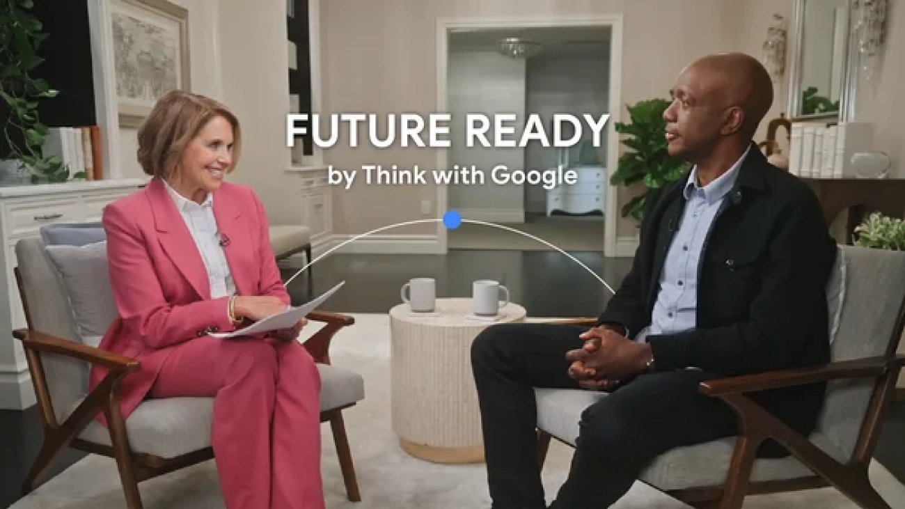
 Katie Couric hosts Future Ready by Think with Google, a new interview series featuring experts in AI, cybersecurity and psychology.
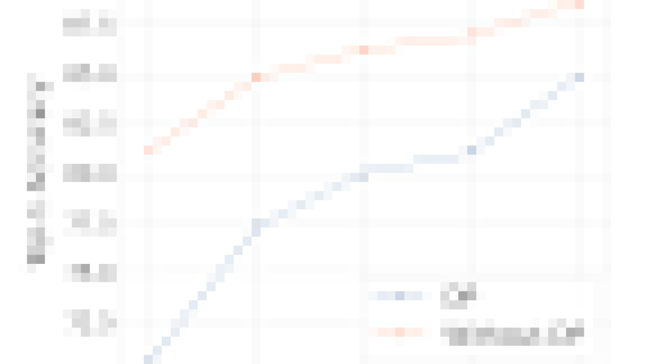


 AI can be hugely beneficial to society if citizens, educators, academics, civil society and governments unite to shape it responsibly.


