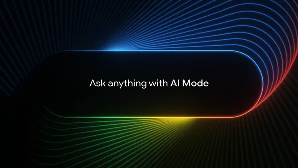
 Anyone in the U.S. can now get immediate access to AI Mode in Labs.Read More

Anyone in the U.S. can now get immediate access to AI Mode in Labs.Read More

 Google is announcing a new paper and support for an effort to train 100,000 electrical workers and 30,000 new apprentices in the United States.Read More

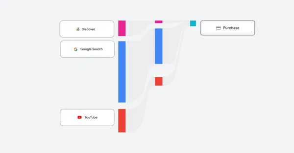 An overview of the latest reporting features, including channel performance reporting, coming to Performance Max.Read More

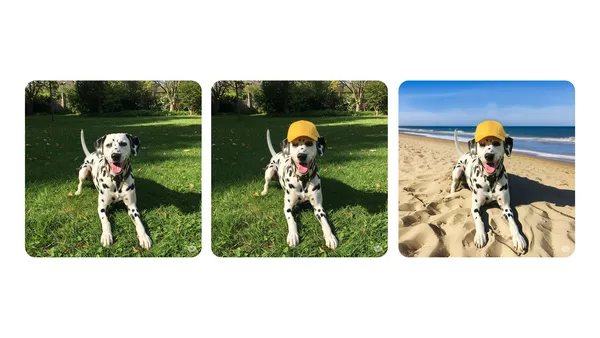 We’re rolling out the ability to easily modify both your AI creations and images you upload from your phone or computer.Read More
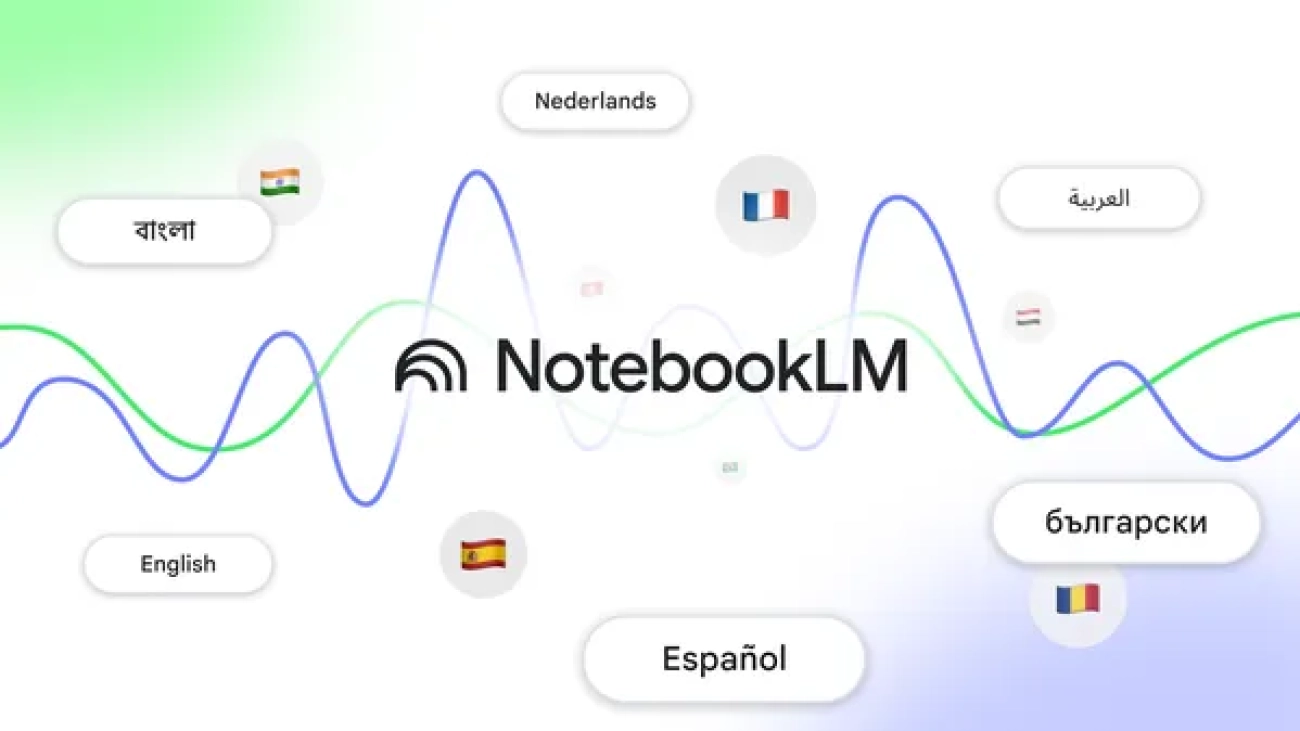
 Learn more about NotebookLM’s Audio Overviews feature and its expansion to more than 50 languages.Read More

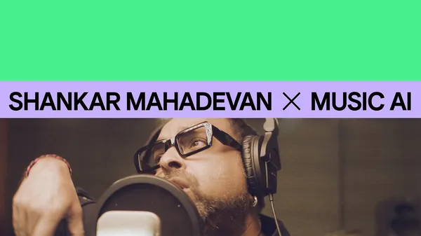 Go behind the scenes in this new Lab Session and learn how Indian music icon Shankar Mahadevan used Music AI Sandbox to help create the song ”Rubaroo”.Read More

 Go behind the scenes on the development of Google Cloud WAN, now available to external customers for the first time.Read More
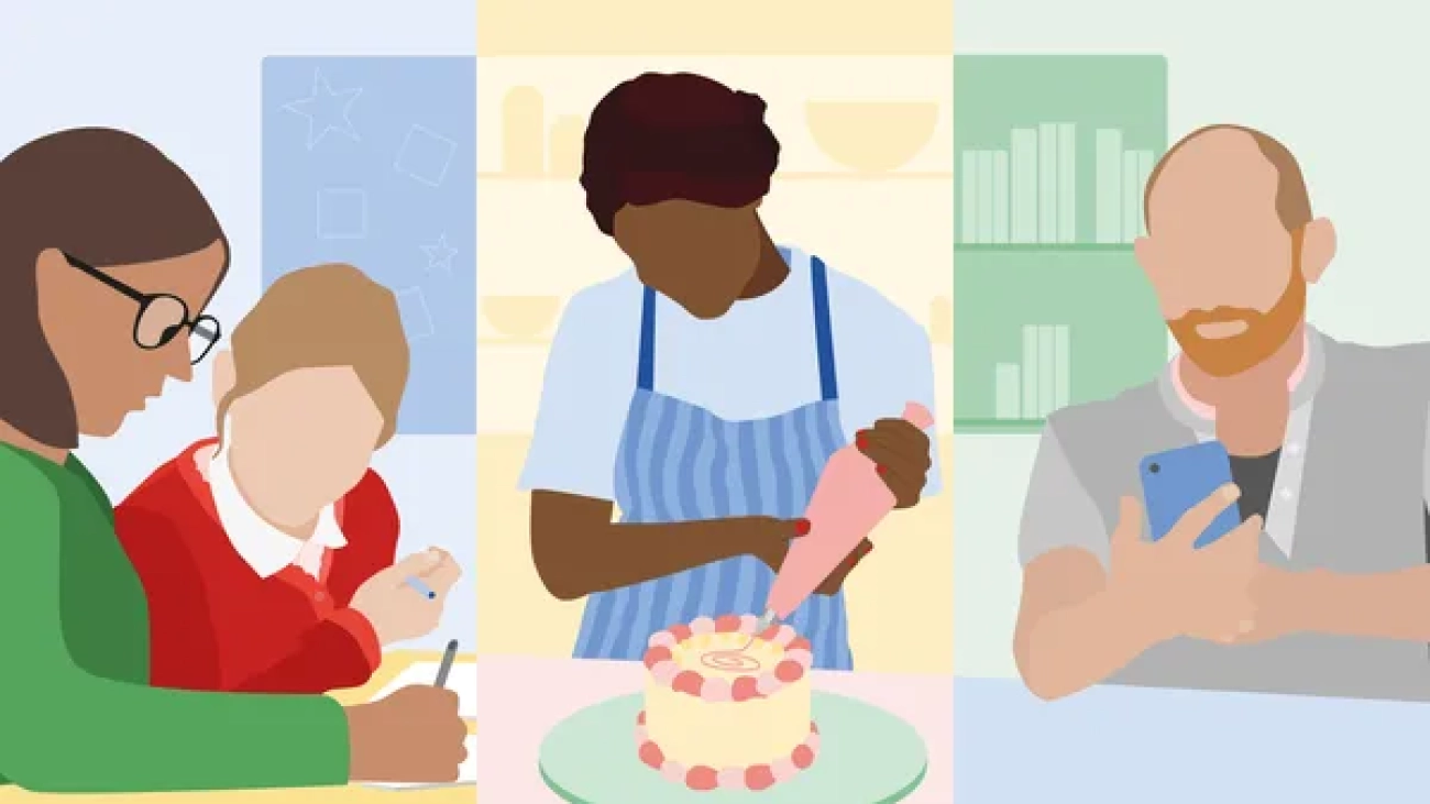
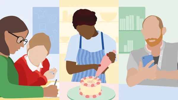 Google’s AI Works report shares how the UK can double AI usage, narrow the AI adoption gap, and boost worker productivity.Read More
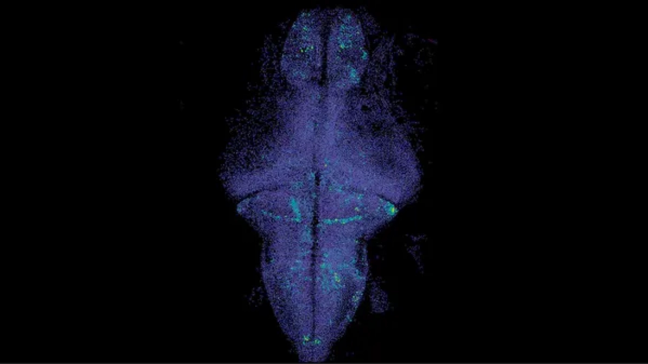
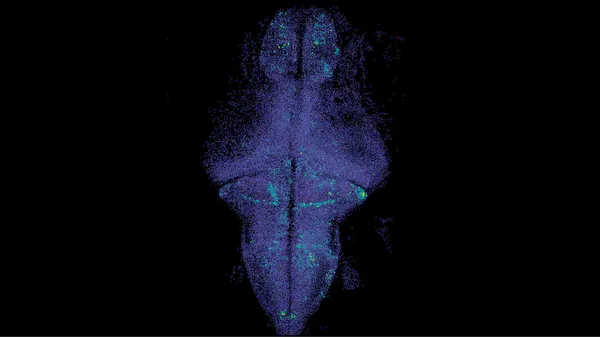 AI could one day help neuroscientists predict activity in the human brain, just like language models can predict the next word in a sentence.After more than a decade of …Read More

 Today, we’re opening applications for this year’s Google for Startups AI Academy: American Infrastructure cohort.Designed for Seed to Series A startups using AI in criti…Read More