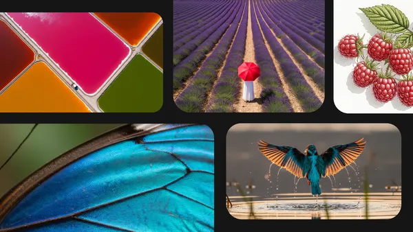
 From Imagen 4 and Veo 3 to Flow, try these new generative media tools today.Read More

From Imagen 4 and Veo 3 to Flow, try these new generative media tools today.Read More

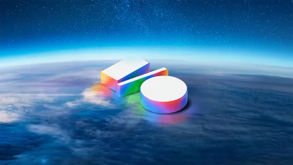
 At I/O 2025, we shared updates to our Gemini 2.5 model series and Deep Think, an experimental enhanced reasoning mode for 2.5 Pro.Read More
 The Gemini app is getting major new updates, from Veo 3 and Imagen 4 to Deep Research and Canvas.Read More

 Today, we’re announcing a partnership between Google DeepMind and Primordial Soup, a new venture dedicated to storytelling innovation founded by pioneering director Darr…Read More

 At Google I/O, we discussed how we’re extending Gemini to become a world model.Read More

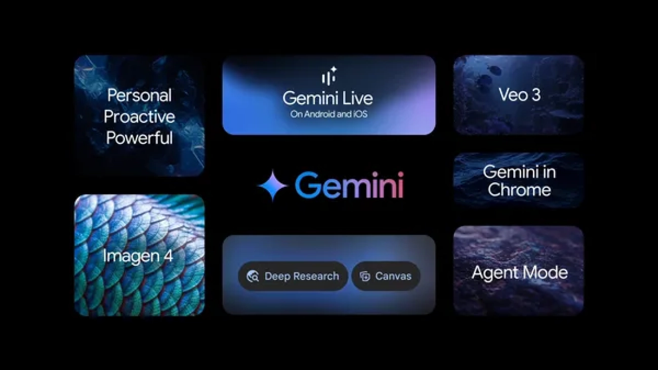
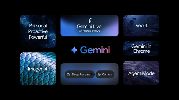
 At our annual developer conference, we announced how we’re making AI even more helpful with Gemini.Read More
 Today at I/O, we showed how we’re enhancing Search with our latest Gemini models via AI Mode.Read More

 Learn about the new SynthID Detector portal we announced at I/O to help people understand how the content they see online was generated.Read More
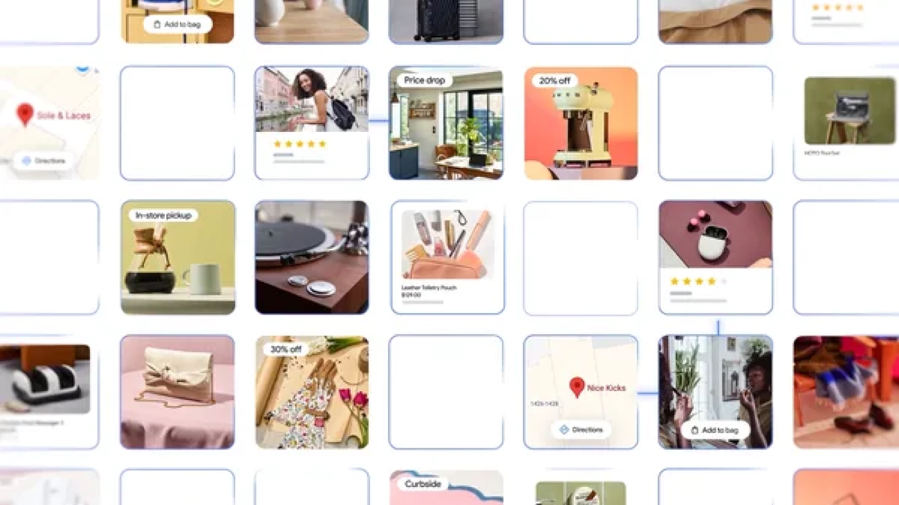
 Learn more about Google’s new shopping features in AI Mode as well as a new virtual try-on tool that works with personal photos.Read More
 We’re launching the new NotebookLM app, designed to help people understand anything, anywhere.Read More