Meta: Less Wright, Hamid Shojanazeri, Vasiliy Kuznetsov, Daniel Vega-Myhre, Gokul Nadathur, Will Constable, Tianyu Liu, Tristan Rice, Driss Guessous, Josh Fromm, Luca Wehrstedt, Jiecao Yu, Sandeep Parab
Crusoe: Ethan Petersen, Martin Cala, Chip Smith
Working with Crusoe.AI we were provided access to one of their new 2K H200 clusters in Iceland, which enabled us to showcase training accelerations of 34 – 43% at scale by leveraging TorchTitan’s HSDP2 and TorchAO’s new float8 rowwise, with comparable convergence and stability vs BF16.

In this post we detail the synergy of H200’s with PyTorch’s new Float8 rowwise training with TorchTitan’s FSDP2/HSDP2 and CP at scale.
Background – what is an H200?
H200’s are an ‘enhanced’ H100, offering the exact same compute as an H100, but with two additional improvements.
- Larger global memory, 141GiB HBM3e vs the standard 80GiB HBM3
- Memory bandwidth is ~43% faster with 4.8TB/s vs 3.35 TB/s. The faster memory transfer has an outsized effect on training speed, especially for PyTorch’s AsyncTP.
What is PyTorch Float8 rowwise?
Float 8 Rowwise is a finer grained resolution for Float8 vs the previous ‘tensor wise’ Float8. It is designed to ensure finer grained accuracy to support larger workloads that tend to become more sensitive to quantization at scale and as training progresses.
There are two key improvements with Float8 rowwise:
- Each row now maintains its own scaling factor versus a single scaling factor for the entire tensor, thus improving quantization precision. Finer grained scaling per row helps reduce the effect of outliers (extreme values that force the quantization scaling factor to stretch and degrade the precision of the normally distributed values) and thus ensures better precision.
- The scaling factor itself is now implemented by rounding down to the nearest power of 2. This has been shown to help reduce quantization errors when multiplying/dividing by the scaling factor as well as ensuring large values remain scaled to the same value in both the forward and backward passes.
Note that other large scale models have been trained using Float8 at 2K scale with a combination of 1×128 groupwise and 128×128 blockwise, with power of 2 scaling factors. They had the same goal of improving Float8’s precision for supporting large scale training.
Thus, Float8 rowwise offers a similar promise to enable Float8 for very large scale training, but we wanted to provide proof of stability and convergence at scale, which training on the Crusoe H200 2k cluster provided initial verification thereof.
Showcasing Float8 Rowwise Loss convergence vs BF16 at 1600 and 1920 GPU Scale:
In order to verify comparable loss convergence, we ran two separate runs at both 1920 and then 1600 (1.6k) gpu scale using TorchTitan and Lllama3 70B. The 1.6K GPU runs were set for 2.5k iterations, using TorchTitans’ HSDP2 and Context Parallel to enable 2D parallelism.
The loss convergence tests were run using Titan’s deterministic mode – this mode effectively freezes most potential sources of variation from run to run, and thus helps ensure that the only substantial change is what we want to test, namely the loss convergence and loss curves of BF16 vs Float8 Rowwise.
Note that deterministic mode also slows down training speed because various kernels will not be autotuned to maximize throughput (otherwise we risk using different kernels between runs and introducing variance).
Two runs were completed, one with BF16 and the other with Float8 Rowwise.
Both runs completed their assigned 2.5k iters without issue, showcasing the Crusoe cluster stability, with FP8 completing at exactly 24 hours and BF16 finishing after 31 hours, 19 minutes.
| DType | Time / Iters | Loss |
| BF16 | 24 hours | 3.15453 |
| Float8 Rowwise | 24 hours | 2.86386 |
| BF16 | 31 hours, 19 minutes / 2.5K | 2.88109 |
| Float8 Rowwise | 24 hours / 2.5K | 2.86386 |
At the 24 hour mark, Float8 completed 2.5K iterations showcasing the comparative speed up (even in deterministic mode) of float8 training. At the 24 hour mark, Float8 enabled a +9.21% relative improvement in loss compared to BF16 for the same 24 hours of large scale training time.
After 31 hours, 19 minutes, the BF16 run finally completed its 2.5k iters.
The final loss numbers:
BF16 = 2.88109
Float8 = 2.86386
From the loss curves we observed very similar curves at the first and last ⅓ and then a turbulent zone in the middle where both showed similar spikes, but with a slight skew to the relative timing of the spikes.

As a result of this, we can see that PyTorch’s Float8 rowwise offers similar convergence but over 33% speedup for the same amount of training time.
Long Term Training stability with Float8 Rowwise
Beyond showcasing comparable convergence, we also wanted to show longer term training stability with Float8 and thus we launched a 4 day, 15K run at 256 scale.

As shown above, Float8 training ran for over 100 hours with no issues, highlighting the long term stability of Float8 Rowwise.
Determinism in TorchTitan
To verify determinism and to see if the spikiness in the longer runs was from scale, we also ran a smaller run comprising of 2 runs of BF16, and 1 run of Float8 at 256 scale, and with HSDP2 only (i.e. without 2D Context parallel).
In this case both BF16 runs had identical curves and final loss, and we saw a similar spikiness zone for all three runs.
At the 2K iteration mark, both Float8 and BF16 ending at nearly identical points:
BF16 *2 = 3.28538
Float8 rowwise = 3.28203

The above result confirms that neither CP nor scale (2k) are responsible for spikiness in the loss as we saw similar effect at 256 scale as well. The most likely explanation for the loss spikes could be content distribution in the dataset.
For the sake of determinism, the experiments were run with a serialized C4 dataset (not shuffled), meaning the spikes could be from encountering new content within the dataset.
Net speedups at various Scales with Float8 rowwise:
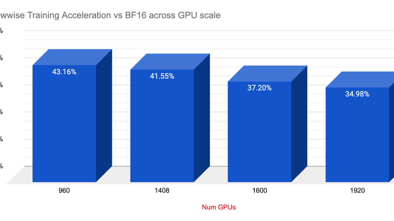
We performed shorter runs at various GPU scales to understand how Float8 Rowwise would scale in terms of training acceleration as cluster sizes expanded. Doubling in scale from 960 to 1920, Float8 continued to deliver impressive training speedups, with a range of over 34-43% gains compared to BF16. We also want to note that scaling from 1k to 2k GPUs communication overhead likely kicked in and we observed a 4% hit on throughput with BF16.

As shown in the longer training runs at scale above, Float8 rowwise delivered substantial speedups with equal or even slightly improved loss endpoints while delivering 34% speedups at 1920 (DeepSeek) scale.
How can I use Float8 Rowwise in my training?
Float8 Rowwise is available now for you to use in your large scale training. It is packaged in TorchAO’s latest builds (0.9 and higher) and integrated into TorchTitan natively if you want to get up and running quickly.
To activate Float8 Rowwise in TorchTitan:
First enable the model converter to hotswap the nn.linears into float8 linear layers in your models .toml file – see line 29:

Secondly, specify the ‘rowwise’ float8 recipe – see line 72:

Note that you have three choices for the ‘recipe_name’:
- rowwise which is the recommended default,
- tensorwise (the older style float8) and
- rowwise_with_gw_hp.
The gw_hp rowwise option keeps the gradients to the weights in BF16 precision during the backwards pass, and this can further enhance float8 precision for extremely sensitive workloads. But, it can ironically be a bit more performant than generic rowwise if the majority of the matmul sizes in your model are smaller (with an estimated tipping point at roughly 13-16K dimensions on H100).
Thus while we recommend rowwise as the default, it may be worth comparing with gw_hp on your model to verify which provides the best performance, with an upside of even greater precision.
By toggling the model converter on and off with a #, you can directly compare training acceleration between BF16 and Float8 Rowwise to understand the potential speedups for your own training.
Future Updates:
We’ll have an additional update coming showcasing multiple improvements for Pipeline Parallel and Async Distributed Checkpointing so please stay tuned.

 A-Series Graphics