Undergraduates develop next-generation intelligence tools

The coronavirus pandemic has driven us apart physically while reminding us of the power of technology to connect. When MIT shut its doors in March, much of campus moved online, to virtual classes, labs, and chatrooms. Among those making the pivot were students engaged in independent research under MIT’s Undergraduate Research Opportunities Program (UROP). 

With regular check-ins with their advisors via Slack and Zoom, many students succeeded in pushing through to the end. One even carried on his experiments from his bedroom, after schlepping his Sphero Bolt robots home in a backpack. “I’ve been so impressed by their resilience and dedication,” says Katherine Gallagher, one of three artificial intelligence engineers at MIT Quest for Intelligence who works with students each semester on intelligence-related applications. “There was that initial week of craziness and then they were right back to work.” Four projects from this spring are highlighted below.

Learning to explore the world with open eyes and ears

Robots rely heavily on images beamed through their built-in cameras, or surrogate “eyes,” to get around. MIT senior Alon Kosowsky-Sachs thinks they could do a lot more if they also used their microphone “ears.” 

From his home in Sharon, Massachusetts, where he retreated after MIT closed in March, Kosowsky-Sachs is training four baseball-sized Sphero Bolt robots to roll around a homemade arena. His goal is to teach the robots to pair sights with sounds, and to exploit this information to build better representations of their environment. He’s working with Pulkit Agrawal, an assistant professor in MIT’s Department of Electrical Engineering and Computer Science, who is interested in designing algorithms with human-like curiosity.

While Kosowsky-Sachs sleeps, his robots putter away, gliding through an object-strewn rink he built for them from two-by-fours. Each burst of movement becomes a pair of one-second video and audio clips. By day, Kosowsky-Sachs trains a “curiosity” model aimed at pushing the robots to become bolder, and more skillful, at navigating their obstacle course.

“I want them to see something through their camera, and hear something from their microphone, and know that these two things happen together,” he says. “As humans, we combine a lot of sensory information to get added insight about the world. If we hear a thunder clap, we don’t need to see lightning to know that a storm has arrived. Our hypothesis is that robots with a better model of the world will be able to accomplish more difficult tasks.”

Training a robot agent to design a more efficient nuclear reactor 

One important factor driving the cost of nuclear power is the layout of its reactor core. If fuel rods are arranged in an optimal fashion, reactions last longer, burn less fuel, and need less maintenance. As engineers look for ways to bring down the cost of nuclear energy, they are eying the redesign of the reactor core.

“Nuclear power emits very little carbon and is surprisingly safe compared to other energy sources, even solar or wind,” says third-year student Isaac Wolverton. “We wanted to see if we could use AI to make it more efficient.” 

In a project with Josh Joseph, an AI engineer at the MIT Quest, and Koroush Shirvan, an assistant professor in MIT’s Department of Nuclear Science and Engineering, Wolverton spent the year training a reinforcement learning agent to find the best way to lay out fuel rods in a reactor core. To simulate the process, he turned the problem into a game, borrowing a machine learning technique for producing agents with superhuman abilities at chess and Go.

He started by training his agent on a simpler problem: arranging colored tiles on a grid so that as few tiles as possible of the same color would touch. As Wolverton increased the number of options, from two colors to five, and four tiles to 225, he grew excited as the agent continued to find the best strategy. “It gave us hope we could teach it to swap the cores into an optimal arrangement,” he says.

Eventually, Wolverton moved to an environment meant to simulate a 36-rod reactor core, with two enrichment levels and 2.1 million possible core configurations. With input from researchers in Shirvan’s lab, Wolverton trained an agent that arrived at the optimal solution.

The lab is now building on Wolverton’s code to try to train an agent in a life-sized 100-rod environment with 19 enrichment levels. “There’s no breakthrough at this point,” he says. “But we think it’s possible, if we can find enough compute resources.”

Making more livers available to patients who need them

About 8,000 patients in the United States receive liver transplants each year, but that’s only half the number who need one. Many more livers might be made available if hospitals had a faster way to screen them, researchers say. In a collaboration with Massachusetts General Hospital, MIT Quest is evaluating whether automation could help to boost the nation’s supply of viable livers.  

In approving a liver for transplant, pathologists estimate its fat content from a slice of tissue. If it’s low enough, the liver is deemed ready for transplant. But there are often not enough qualified doctors to review tissue samples on the tight timeline needed to match livers with recipients. A shortage of doctors, coupled with the subjective nature of analyzing tissue, means that viable livers are inevitably discarded.

This loss represents a huge opportunity for machine learning, says third-year student Kuan Wei Huang, who joined the project to explore AI applications in health care. The project involves training a deep neural network to pick out globules of fat on liver tissue slides to estimate the liver’s overall fat content.

One challenge, says Huang, has been figuring out how to handle variations in how various pathologists classify fat globules. “This makes it harder to tell whether I’ve created the appropriate masks to feed into the neural net,” he says. “However, after meeting with experts in the field, I received clarifications and was able to continue working.”

Trained on images labeled by pathologists, the model will eventually learn to isolate fat globules in unlabeled images on its own. The final output will be a fat content estimate with pictures of highlighted fat globules showing how the model arrived at its final count. “That’s the easy part — we just count up the pixels in the highlighted globules as a percentage of the overall biopsy and we have our fat content estimate,” says the Quest’s Gallagher, who is leading the project.

Huang says he’s excited by the project’s potential to help people. “Using machine learning to address medical problems is one of the best ways that a computer scientist can impact the world.”

Exposing the hidden constraints of what we mean in what we say

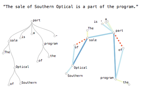
Language shapes our understanding of the world in subtle ways, with slight variations in the words we use conveying sharply different meanings. The sentence, “Elephants live in Africa and Asia,” looks a lot like the sentence “Elephants eat twigs and leaves.” But most readers will conclude that the elephants in the first sentence are split into distinct groups living on separate continents but not apply the same reasoning to the second sentence, because eating twigs and eating leaves can both be true of the same elephant in a way that living on different continents cannot.

Karen Gu is a senior majoring in computer science and molecular biology, but instead of putting cells under a microscope for her SuperUROP project, she chose to look at sentences like the ones above. “I’m fascinated by the complex and subtle things that we do to constrain language understanding, almost all of it subconsciously,” she says.

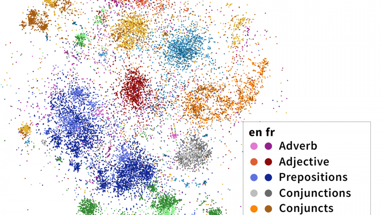
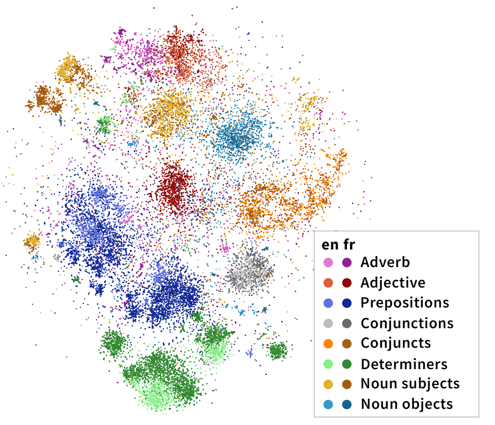
Working with Roger Levy, a professor in MIT’s Department of Brain and Cognitive Sciences, and postdoc MH Tessler, Gu explored how prior knowledge guides our interpretation of syntax and ultimately, meaning. In the sentences above, prior knowledge about geography and mutual exclusivity interact with syntax to produce different meanings.

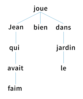
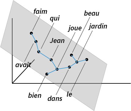
After steeping herself in linguistics theory, Gu built a model to explain how, word by word, a given sentence produces meaning. She then ran a set of online experiments to see how human subjects would interpret analogous sentences in a story. Her experiments, she says, largely validated intuitions from linguistic theory.

One challenge, she says, was having to reconcile two approaches for studying language. “I had to figure out how to combine formal linguistics, which applies an almost mathematical approach to understanding how words combine, and probabilistic semantics-pragmatics, which has focused more on how people interpret whole utterances.’ “

After MIT closed in March, she was able to finish the project from her parents’ home in East Hanover, New Jersey. “Regular meetings with my advisor have been really helpful in keeping me motivated and on track,” she says. She says she also got to improve her web-development skills, which will come in handy when she starts work at Benchling, a San Francisco-based software company, this summer.

Spring semester Quest UROP projects were funded, in part, by the MIT-IBM Watson AI Lab and Eric Schmidt, technical advisor to Alphabet Inc., and his wife, Wendy.

Read More

Finding Cross-Lingual Syntax in Multilingual BERT

Finding Cross-Lingual Syntax in Multilingual BERT

We projected head-dependent pairs from both English (light colors) and French (dark colors) into a syntactic space trained on solely English mBERT representations. Both English and French head-dependent vectors cluster; dependencies of the same label in both English and French share the same cluster. Although our method has no access to dependency labels, the dependencies exhibit cross-lingual clustering that largely agree with linguists’ categorizations.

If you ask a deep neural network to read a large number of languages, does it share what it’s learned about sentence structure between different languages?

Deep neural language models like BERT have recently demonstrated a fascinating level of understanding of human language. Multilingual versions of these models, like Multilingual BERT (mBERT), are able to understand a large number of languages simultaneously. To what extent do these models share what they’ve learned between languages?

Focusing on the syntax, or grammatical structure, of these languages, we show that Multilingual BERT is able to learn a general syntactic structure applicable to a variety of natural languages. Additionally, we find evidence that mBERT learns cross-lingual syntactic categories like “subject” and “adverb”—categories that largely agree with traditional linguistic concepts of syntax! Our results imply that simply by reading a large amount of text, mBERT is able to represent syntax—something fundamental to understanding language—in a way that seems to apply across many of the languages it comprehends.

More specifically, we present the following:

  • We apply the structural probe method of Hewitt and Manning (2019) to 10 languages, finding syntactic subspaces in a multilingual setting.

  • Through zero-shot transfer experiments, we demonstrate that mBERT represents some syntactic features in syntactic subspaces that overlap between languages.

  • Through an unsupervised method, we find that mBERT natively represents dependency clusters that largely overlap with the UD standard.

Our results are presented in the forthcoming ACL 2020 paper, Finding Universal Grammatical Relations in Multilingual BERT. This post draws from the paper, which is joint work with John Hewitt and Chris Manning. You can also find the code here.

If you’d like to skip the background and jump to the discussion of our methods, click here. Otherwise, read on!

Learning Languages

Past childhood, humans usually learn a language by comparison to one we already speak.1 We naturally draw parallels between sentences with similar meanings—for example, after learning some French, one can work out that Je vis le chat mignon is essentially a word-for-word translation of I see the cute cat. Importantly, humans draw parallels in syntax, or the way words are organized to form meaning; most bilinguals know that mignon is an adjective which describes the noun chat, just as cute describes the noun cat—even though the words are in the opposite order between languages.

How do we train a neural network to understand multiple languages at the same time? One intuitive approach might be to equip the neural network with a multilingual dictionary and a list of rules to transfer between one language to another. (For example, adjectives come before the noun in English but after the noun in Khmer.) However, mirroring recent developments in monolingual neural networks, one more recent method is to give our neural network enormous amounts of data in multiple languages. In this approach, we never provide even a single translation pair, much less a dictionary or grammar rules.

Surprisingly, this trial by fire works! A network trained this way, like Google’s Multilingual BERT, is able to understand a vast number of languages beyond what any human can handle, even a typologically divergent set ranging from English to Hindi to Indonesian.

This raises an interesting question: how do these networks understand multiple languages at the same time? Do they learn each language separately, or do they draw parallels between the way syntax works in different languages?

Knowing What it Means to “Know”

First, let’s ask: what does it even mean for a neural network to “understand” a linguistic property?

One way to evaluate this is through the network’s performance on a downstream task, such as a standard leaderboard like the GLUE (General Language Understanding Evaluation) benchmark. By this metric, large models like BERT do pretty well! However, although high performance numbers suggest in some sense that the model understands some aspects of language generally speaking, they conflate the evaluation of many different aspects of language, and it’s difficult to test specific hypotheses about the individual properties of our model.

Instead, we use a method known as probing. The central idea is as follows: we feed linguistic data for which we know the property we’re interested in exploring (e.g. part-of-speech) through the network we want to probe. Instead of looking at the predictions of the model themselves, for each sentence we feed through, we save the hidden representations, which one can think of as the model’s internal data structures. We then train a probe—a secondary model—to recover the target property from these representations, akin to how a neuroscientist might read out emotions from a MRI scan of your brain.

Probes are usually designed to be simple, to test what the neural network makes easily accessible. intuitively, the harder we try to tease a linguistic property out of the representations, the less the representations themselves matter to your final results. As an example, we might be able to build an extremely complex model to predict whether someone is seeing a cat, based on the raw data coming from the retina; however, this doesn’t mean that the retina itself intrinsically “understands” what a cat is.2

A Tale of Syntax and Subspaces

So what form, exactly, do these hidden representations take? The innards of a neural network like BERT represent each sentence as a series of real-valued vectors (in real life, these are 768-dimensional, but we’ve represented them as three-dimensional here):

A probe, then, is a model that maps from a word vector to some linguistic property of interest. For something like part of speech, this might take the form of a 1-layer neural classifier which predicts a category (like noun or verb).

But how do we evaluate whether a neural network knows something as nebulous as syntax, the way words and phrases are arranged to create meaning? Linguists believe sentences are implicitly organized into syntax trees, which we generate mentally in order to produce a sentence. Here’s an example of what that looks like:

Syntax tree for French Jean qui avait faim joue bien dans le jardin (Jean, who was hungry, plays in the garden).

To probe whether BERT encodes a syntax tree internally, we apply the structural probe method [Hewitt and Manning, 2019]. This finds a linear transformation3 such that the tree constructed by connecting each word to the word closest to it approximates a linguist’s idea of what the parse tree should look like. This ends up looking like this:

Intuitively, we can think of BERT vectors as lying in a 768-dimensional space; the structural probe tries to find a linear subspace of the BERT space which best recovers syntax trees.

Does this work, you might ask? Well, this certainly seems to be the case:

A gold parse tree annotated by a linguist, and a parse tree generated from Monolingual BERT embeddings. From Coenen et al. (2019).

Hewitt and Manning apply this method only to monolingual English BERT; we apply their method to 10 other languages, finding that mBERT encodes syntax to various degrees in all of them. Here’s a table of performance (measured in UUAS, or unlabeled undirected accuracy score) as graphed against the rank of the probe’s linear transformation:

Probing for Cross-Lingual Syntax

With this in mind, we can turn to the question with which we started this blog post:

Does Multilingual BERT represent syntax similarly cross-lingually?

To answer this, we train a structural probe to predict syntax from representations in one language—say, English—and evaluate it on another, like French. If a probe trained on mBERT’s English representations performs well when evaluated on French data, this intuitively suggests that the way mBERT encodes English syntax is similar to the way it encodes French syntax.

Does this work? In a word, basically:

Syntactic trees for a single English sentence generated by structural probes trained on English, French, and Indonesian data.
Black represents the reference syntactic tree as defined by a linguist.
The English structural probe is almost entirely able to replicate the syntactic tree, with one error;
the French probe finds most of the syntactic tree, while the Indonesian probe is able to recover the high-level structure but misses low-level details.

Out of the 11 languages that we evaluate on, we find that probes trained on representations from one language are able to successfully recover syntax trees—to varying degrees—in data from another language. Evaluated on two numerical metrics of parse tree accuracy, applying probes cross-lingually performs surprisingly well! This performance suggests that syntax is encoded similarly in mBERT representations across many different languages.

UUAS DSpr.
Best baseline 0% 0%
Transfer from best source language 62.3% 73.1%
Transfer from holdout subspace (trained on all languages other than eval) 70.5% 79%
Transfer from subspace trained on all languages (including eval) 88.0% 89.0%
Training on evaluation language directly 100% 100%
Table: Improvement for various transfer methods over best baseline, evaluated on two metrics: UUAS (unlabeled undirected accuracy score) and DSpr. (Spearman correlation of tree distances). Percent improvement is calculated with respect to the total possible improvement in recovering syntactic trees over baseline (as represented by in-language supervision.)

Finding Universal Grammatical Relations in mBERT

We’ve shown that cross-lingual syntax exists—can we visualize it?

Recall that the structural probe works by finding a linear subspace optimized to encode syntax trees. Intuitively, this syntactic subspace might focus on syntactic aspects of mBERT’s representations. Can we visualize words in this subspace and get a first-hand view of how mBERT represents syntax?

One idea is to focus on the edges of our syntactic tree, or head-dependent pairs. For example, below, was is the head of the dependent chef:

Let’s try to visualize these vectors in the syntactic subspace and see what happens! Define the head-dependent vector as the vector between the head and the dependent in the syntactic subspace:

We do this for every head-dependent pair in every sentence in our corpus, then visualize the resulting 32-dimensional vectors in two dimensions using t-SNE, a dimensionality reduction algorithm. The results are striking: the dependencies naturally separate into clusters, whose identities largely overlap with the categories that linguists believe are fundamental to language! In the image below, we’ve highlighted the clusters with dependency labels from Universal Dependencies, like amod (adjective modifying a noun) and conj (two clauses joined by a coordinating conjunction like and, or):

Importantly, these categories are multilingual. In the above diagram, we’ve projected head-dependent pairs from both English (light colors) and French (dark colors) into a syntactic space trained on solely English mBERT representations. We see that French head-dependent vectors cluster as well, and that dependencies with the same label in both English and French share the same cluster.

Freedom from Human-Chosen Labels

The fact that BERT “knows” dependency labels is nothing new; previous studies have shown high accuracy in recovering dependency labels from BERT embeddings. So what’s special about our method?

Training a probe successfully demonstrates that we can map from mBERT’s representations to a standard set of dependency category labels. But because our probe needs supervision on a labeled dataset, we’re limited to demonstrating the existence of a mapping to human-generated labels. In other words, probes make it difficult to gain insight into the categories drawn by mBERT itself.

By contrast, the structural probe never receives information about what humans think dependency label categories should look like. Because we only ever pass in head-dependent pairs, rather than the category labels associated with these pairs, our method is free from human category labels. Instead, the clusters that emerge from the data are a view into mBERT’s innate dependency label representations.4

For more work on the latent linguistic ontology of BERT, see: Michael et al. (2020) and Limisiewicz et al. (2020).

Analyzing mBERT’s Internal Representations

Taking a closer look, what can we discover about how mBERT categorizes head-dependency relations, as compared to human labels? Our results show that mBERT draws slightly different distinctions from Universal Dependencies. Some are linguistically valid distinctions not distinguished by the UD standards, while others are more influenced by word order, separating relations that most linguists would group together. Here’s a brief overview:

t-SNE visualization of 100,000 syntactic difference vectors projected into the cross-lingual syntactic subspace of Multilingual BERT. We exclude `punct` and visualize the top 11 dependencies remaining, which are collectively responsible for 79.36% of the dependencies in our dataset. Clusters of interest highlighted in yellow; linguistically interesting clusters labeled.
  • Adjectives: We find that mBERT breaks adjectives into two categories: prenominal adjectives in cluster (b) (e.g., Chinese 獨特的地理) and postnominal adjectives in cluster (u) (e.g., French applications domestiques).

  • Nominal arguments: mBERT maintains the UD distinction between subject and object. However, indirect objects cluster with direct objects; other adjuncts cluster with subjects if near the beginning of a sentence and obj otherwise. This suggests that mBERT categorizes nominal arguments into pre-verbal and post-verbal categories.

  • Relative clauses In the languages in our dataset, there are two major ways of forming relative clauses. Relative pronouns (e.g., English the man who is hungry are classed by Universal Dependencies as being an nsubj dependent, while subordinating markers (e.g., English I know that she saw me) are classed as the dependent of a mark relation. However, mBERT groups both of these relations together, clustering them distinctly from most nsubj and mark relations.

  • Determiners The linguistic category of determiners (det) is split into definite articles (i), indefinite articles (e), possessives (f), and demonstratives (g). Sentence-initial definite articles (k) cluster separately from other definite articles (j).

  • Expletive subjects Just as in UD, expletive subjects, or third person pronouns with no syntactic meaning (e.g. English It is cold, French Il faudrait, Indonesian Yang menjadi masalah kemudian), cluster separately (k) from other nsubj relations (small cluster in the bottom left).

Conclusion

In this work, we’ve found that BERT shares some of the ways it represents syntax between its internal representations of different languages. We’ve provided evidence that mBERT learns natural syntactic categories that overlap cross-lingually. Interestingly, we also find evidence that these categories largely agree with traditional linguistic concepts of syntax.

Excitingly, our methods allow us to examine fine-grained syntactic categories native to mBERT. By removing assumptions on what the ontology of syntactic relations should look like, we discover that mBERT’s internal representations innately share significant overlap with linguists’ idea of what syntax looks like. However, there are also some interesting differences between the two, the nature of which is definitely worth further investigation!

If you’d like to run some tests or generate some visualizations of your own, please head on over to the multilingual-probing-visualization codebase!

Finally, I’m deeply grateful to John Hewitt and Chris Manning, as well as members of the Stanford NLP group for their advice, including but not limited to: Erik Jones, Sebastian Schuster, and Chris Donahue. Many thanks also to John Hewitt and Dylan Losey for reading over the draft of this blog post, and to Mohammad Rasooli for advice on Farsi labels in the original paper.

  1. For a linguistic perspective (specifically, in the field of second-language acquisition), see Cook (1995)

  2. This definition is a general overview and leaves some important questions. How exactly, for instance, do we evaluate the complexity of our probe? Relatedly, how much of the performance improvement is due to the model, and how much is due to the probe itself? For more work on this, see Hewitt and Liang (2019) and Pimentel et al. (2020)

  3. A linear transformation on a vector is simply multiplication by a matrix:  

  4. Technically speaking, this is constrained to the assumption that BERT would choose the same head-dependent pairs as UD does. 

Read More

Microsoft President Brad Smith talks data, Covid-19, and a potential “digital 9/11”

In a virtual discussion hosted by MIT last week, viewers learned that there are many problems that concern Microsoft President Brad Smith: things like climate change, Covid-19, and the work of the future.

Attendees also learned how seriously he takes the issue of computer security: 45 minutes into the event, his Windows system automatically rebooted for a lightning-quick software update.

“There are a lot of benefits to working from home,” he said with a laugh after rejoining, “but it certainly also adds a level of unpredictability.”

Smith’s conversation with MIT Professor Daniela Rus on May 14 spanned a wide range of topics, from the challenges of Covid-19 to the security of online voting. The fireside chat was held as part of MIT’s “Hot Topics in Computing” series, founded by the Computer Science and Artificial Intelligence Laboratory (CSAIL). The series is now an Institute-wide effort being co-presented with the MIT Stephen A. Schwarzman College of Computing (SCC). SCC Dean Dan Huttenlocher opened the event with a welcome to the audience and introduced Smith and Rus.

Having worked at Microsoft for 25 years and served as its president since 2015, Smith gave an inside look at what it’s been like to be there in recent months — and what the tech company has done to try to help curb the spread of Covid-19. 

In March, for example, Microsoft developed a chatbot to help people determine if they might need a Covid-19 test. Within weeks of deploying the app at a hospital in Seattle, Washington, the company started rolling it out more broadly. The chatbot was ultimately used 190 million times in April, and is now available at 1,500 institutions across 23 countries. 

Smith also discussed the promising work being done with Bluetooth-based contact tracing, but expressed skepticism that it could be adopted at a meaningful scale.

“Not everyone is going to walk around with an app on their phone,” he said. “I think we should recognize that it is a tool, and not a panacea.”

Smith and his colleague Carol Ann Browne recently co-wrote the book “Tools and Weapons,” which examines the promise and peril of technology for both good and bad. The authors draw on lessons in history, from Edward Snowden’s revelations about government surveillance to the Cambridge Analytica scandal, to explore the future of technology and how it needs to be managed. 

While he agreed with Rus’ assessment of the book as one “where the geeks are the heroes,” Smith also warned of the dangers of a future “digital 9/11” with respect to the electric grid and future presidential elections. 

“You don’t need to be a PhD in computer science to have an important role to play,” he said. “As consumers, citizens, and voters, we’re at a point of time where we’d all benefit from being better informed.” 

The long-time sustainability advocate also spoke about Microsoft’s ambitious goals to not just be carbon-negative by 2030, but to remove all of the carbon that the company has emitted since 1975 in the next 30 years. At a higher level, Smith advocated for making what he calls “the biggest R&D investment of our century” to develop new techniques to remove carbon from the environment. 

“We’re going to need huge breakthroughs in the next three decades if we are going to achieve this fundamental goal of protecting the planet the way we need to,” he said.

In the hourlong conversation, Smith often implored his audience of computer scientists and technologists to recognize the responsibility they have to solve tangible real-world problems. He pointed out that, for all the buzz about big data over the last 20 years, the Covid-19 pandemic has actually led to government officials making decisions directly informed by data.

“Data is running the economy and deciding who can leave their house and who needs to stay home,” Smith said. “The world will need the kind of technology that we can create … [and] you all have an opportunity to make a more positive impact in the world than perhaps any generation of MIT students has had before. How can that not get you excited about getting up in the morning?”

Read More

Open-Sourcing BiT: Exploring Large-Scale Pre-training for Computer Vision

Open-Sourcing BiT: Exploring Large-Scale Pre-training for Computer Vision

Posted by Lucas Beyer and Alexander Kolesnikov, Research Engineers, Google Research, Zürich

A common refrain for computer vision researchers is that modern deep neural networks are always hungry for more labeled data — current state-of-the-art CNNs need to be trained on datasets such as OpenImages or Places, which consist of over 1M labelled images. However, for many applications, collecting this amount of labeled data can be prohibitive to the average practitioner.

A common approach to mitigate the lack of labeled data for computer vision tasks is to use models that have been pre-trained on generic data (e.g., ImageNet). The idea is that visual features learned on the generic data can be re-used for the task of interest. Even though this pre-training works reasonably well in practice, it still falls short of the ability to both quickly grasp new concepts and understand them in different contexts. In a similar spirit to how BERT and T5 have shown advances in the language domain, we believe that large-scale pre-training can advance the performance of computer vision models.

In “Big Transfer (BiT): General Visual Representation Learning” we devise an approach for effective pre-training of general features using image datasets at a scale beyond the de-facto standard (ILSVRC-2012). In particular, we highlight the importance of appropriately choosing normalization layers and scaling the architecture capacity as the amount of pre-training data increases. Our approach exhibits unprecedented performance adapting to a wide range of new visual tasks, including the few-shot recognition setting and the recently introduced “real-world” ObjectNet benchmark. We are excited to share the best BiT models pre-trained on public datasets, along with code in TF2, Jax, and PyTorch. This will allow anyone to reach state-of-the-art performance on their task of interest, even with just a handful of labeled images per class.

Pre-training
In order to investigate the effect of data scale, we revisit common design choices of the pre-training setup (such as normalizations of activations and weights, model width/depth and training schedules) using three datasets: ILSVRC-2012 (1.28M images with 1000 classes), ImageNet-21k (14M images with ~21k classes) and JFT (300M images with ~18k classes). Importantly, with these datasets we concentrate on the previously underexplored large data regime.

We first investigate the interplay between dataset size and model capacity. To do this we train classical ResNet architectures, which perform well, while being simple and reproducible. We train variants from the standard 50-layer deep “R50x1” up to the 4x wider and 152-layer deep “R152x4” on each of the above-mentioned datasets. A key observation is that in order to profit from more data, one also needs to increase model capacity. This is exemplified by the red arrows in the left-hand panel of the figure below

Left: In order to make effective use of a larger dataset for pre-training, one needs to increase model capacity. The red arrows exemplify this: small architectures (smaller point) become worse when pre-trained on the larger ImageNet-21k, whereas the larger architectures (larger points) improve. Right: Pre-training on a larger dataset alone does not necessarily result in improved performance, e.g., when going from ILSVRC-2012 to the relatively larger ImageNet-21k. However, by also increasing the computational budget and training for longer, the performance improvement is pronounced.

A second, even more important observation, is that the training duration becomes crucial. If one pre-trains on a larger dataset without adjusting the computational budget and training longer, performance is likely to become worse. However, by adapting the schedule to the new dataset, the improvements can be significant.

During our exploration phase, we discovered another modification crucial to improving performance. We show that replacing batch normalization (BN, a commonly used layer that stabilizes training by normalizing activations) with group normalization (GN) is beneficial for pre-training at large scale. First, BN’s state (mean and variance of neural activations) needs adjustment between pre-training and transfer, whereas GN is stateless, thus side-stepping this difficulty. Second, BN uses batch-level statistics, which become unreliable with small per-device batch sizes that are inevitable for large models. Since GN does not compute batch-level statistics, it also side-steps this issue. For more technical details, including the use of a weight standardization technique to ensure stable behavior, please see our paper.

Summary of our pre-training strategy: take a standard ResNet, increase depth and width, replace BatchNorm (BN) with GroupNorm and Weight Standardization (GNWS), and train on a very large and generic dataset for many more iterations.

Transfer Learning
Following the methods established in the language domain by BERT, we fine-tune the pre-trained BiT model on data from a variety of “downstream” tasks of interest, which may come with very little labeled data. Because the pre-trained model already comes with a good understanding of the visual world, this simple strategy works remarkably well.

Fine-tuning comes with a lot of hyper-parameters to be chosen, such as learning-rate, weight-decay, etc. We propose a heuristic for selecting these hyper-parameters that we call “BiT-HyperRule”, which is based only on high-level dataset characteristics, such as image resolution and the number of labeled examples. We successfully apply the BiT-HyperRule on more than 20 diverse tasks, ranging from natural to medical images.

Once the BiT model is pre-trained, it can be fine-tuned on any task, even if only few labeled examples are available.

When transfering BiT to tasks with very few examples, we observe that as we simultaneously increase the amount of generic data used for pre-training and the architecture capacity, the ability of the resulting model to adapt to novel data drastically improves. On both 1-shot and 5-shot CIFAR (see Fig below) increasing model capacity yields limited returns when pre-training on ILSVRC (green curves). Yet, with large-scale pre-training on JFT, each step-up in model capacity yields massive returns (brown curves), up to BiT-L which attains 64% 1-shot and 95% 5-shot.

The curves depict median accuracy over 5 independent runs (light points) when transferring to CIFAR-10 with only 1 or 5 images per class (10 or 50 images total). It is evident that large architectures pre-trained on large datasets are significantly more data-efficient.

In order to verify that this result holds more generally, we also evaluate BiT on VTAB-1k, which is a suite of 19 diverse tasks with only 1000 labeled examples per task. We transfer the BiT-L model to all these tasks and achieve a score of 76.3% overall, which is a 5.8% absolute improvement over the previous state-of-the-art.

We show that this strategy of large-scale pre-training and simple transfer is effective even when a moderate amount of data is available by evaluating BiT-L on several standard computer vision benchmarks such as Oxford Pets and Flowers, CIFAR, etc. On all of these, BiT-L matches or surpasses state-of-the-art results. Finally, we use BiT as a backbone for RetinaNet on the MSCOCO-2017 detection task and confirm that even for such a structured output task, using large-scale pre-training helps considerably.

Left: Accuracy of BiT-L compared to the previous state-of-the-art general model on various standard computer vision benchmarks. Right: Results in average precision (AP) of using BiT as backbone for RetinaNet on MSCOCO-2017.

It is important to emphasize that across all the different downstream tasks we consider, we do not perform per-task hyper-parameter tuning and rely on the BiT-HyperRule. As we show in the paper, even better results can be achieved by tuning hyperparameters on sufficiently large validation data.

Evaluation with ObjectNet
To further assess the robustness of BiT in a more challenging scenario, we evaluate BiT models that were fine-tuned on ILSVRC-2012 on the recently introduced ObjectNet dataset. This dataset closely resembles real-world scenarios, where objects may appear in atypical context, viewpoint, rotation, etc. Interestingly, the benefit from data and architecture scale is even more pronounced with the BiT-L model achieving unprecedented top-5 accuracy of 80.0%, an almost 25% absolute improvement over the previous state-of-the-art.

Results of BiT on the ObjectNet evaluation dataset. Left: top-5 accuracy, right: top-1 accuracy.

Conclusion
We show that given pre-training on large amounts of generic data, a simple transfer strategy leads to impressive results, both on large datasets as well as tasks with very little data, down to a single image per class. We release the BiT-M model, a R152x4 pre-trained on ImageNet-21k, along with colabs for transfer in Jax, TensorFlow2, and PyTorch. In addition to the code release, we refer the reader to the hands-on TensorFlow2 tutorial on how to use BiT models. We hope that practitioners and researchers find it a useful alternative to commonly used ImageNet pre-trained models.

Acknowledgements
We would like to thank Xiaohua Zhai, Joan Puigcerver, Jessica Yung, Sylvain Gelly, and Neil Houlsby who have co-authored the BiT paper and been involved in all aspects of its development, as well as the Brain team in Zürich. We also would like to thank Andrei Giurgiu for his help in debugging input pipelines. We thank Tom Small for creating the animations used in this blogpost. Finally, we refer the interested reader to the related approaches in this direction by our colleagues in Google Research, Noisy Student, as well as Facebook Research’s highly relevant Exploring the Limits of Weakly Supervised Pretraining.

Galaxy Zoo: Classifying Galaxies with Crowdsourcing and Active Learning

Galaxy Zoo: Classifying Galaxies with Crowdsourcing and Active Learning

A guest article by Mike Walmsley, University of Oxford

The way we do science is changing; there’s exponentially more data every day but around the same number of scientists. The traditional approach of collecting data samples, looking through them, and drawing some conclusions about each one is often inadequate.

One solution is to deploy algorithms to process the data automatically. Another solution is to deploy more eyeballs: recruit members of the public to join in and help. I work on the intersection between the two – combining crowdsourcing and machine learning to do better science than with either alone.

In this article, I want to share how I’ve been using crowdsourcing and machine learning to investigate how galaxies evolve by classifying millions of galaxy images. Along the way, I’ll share some techniques we use to train CNNs that make predictions with uncertainty. I’ll also explain how to use those predictions to do active learning: labelling only the data which would best help you improve your models.

Better Telescopes, Bigger Problems

Ever since Edwin Hubble in the 1920’s, astronomers have looked up at galaxies and tried to classify them into different types – smooth galaxies, spiral galaxies, and so on. But the number of galaxies kept on climbing. About 20 years ago, a grad student named Kevin Schawinski sat at his desk with a pile of 900,000 galaxy pictures, put his head in his hands and thought – “there has to be a better way” than classifying every one himself. He wasn’t alone. To classify all 900,000 galaxies without sacrificing Kevin’s sanity, a team of scientists (including Kevin) built Galaxy Zoo.

Galaxy Zoo is a website that asks members of the public to classify galaxies for us. We show you a galaxy, and we ask simple questions about what you can see, like – is the galaxy smooth, or featured? As you answer, we lead you down a decision tree where the questions depend on how you’ve previously responded.

The Galaxy Zoo UI. Check it out, and join in with the science, here.

Since launch, hundreds of thousands of volunteers have classified millions of galaxies – advancing our understanding of supermassive black holes, spiral arms, the births and deaths of stars, and much more. However, there’s a problem: humans don’t scale. Galaxy surveys keep getting bigger, but we will always have about the same number of volunteers. The latest space-based telescopes can image hundreds of millions of galaxies – far more than we could ever label with crowdsourcing alone.

To keep up, we used TensorFlow to build a galaxy classifier. Other researchers have used the responses we’ve collected to train convolutional neural networks (CNNs) – a type of deep learning model tailored for image recognition. However, traditional CNNs have a drawback; they don’t easily handle uncertainty.

Training a CNN to solve a regression problem by predicting a value for each label and minimising the mean squared error, as is common, implicitly assumes that all labels are equally uncertain – which is definitely not the case for Galaxy Zoo. Further, the CNN only gives a ‘best guess’ answer with no error bars – making it difficult to draw scientific conclusions.

In our paper, we use Bayesian CNNs for morphology classification. Bayesian CNNs provide two key improvements:

  1. They account for varying uncertainty when learning from volunteer responses.
  2. They predict full posteriors over the morphology of each galaxy.

Using our Bayesian CNN, we can learn from noisy labels and make reliable predictions (with error bars) for hundreds of millions of galaxies.

How Bayesian Convolutional Neural Networks Work

There are two key steps to creating our Bayesian CNNs.
1. Predict the parameters of a probability distribution, not the label itself
Training neural networks is much like any other fitting problem: you tweak the model to match the observations. If you are equally confident in all your collected labels, you can just minimise the difference (e.g. mean squared error) between your predictions and the observed values. However for Galaxy Zoo, many labels are more confident than others.
If I observe that, for some galaxy, 30% of volunteers say “bar”, my confidence in that 30% depends heavily on how many people replied – was it 4 or 40? Instead, we predict the probability that a typical volunteer will say “Bar”, and minimise how surprised we should be given the total number of volunteers who replied.
This way, our model understands that errors on galaxies where many volunteers replied are worse than errors on galaxies where few volunteers replied – letting it learn from every galaxy.
In our case, we can model our surprise with the Binomial distribution by recognising that k “Bar” responses from N volunteers is much like k successes from N independent trials.

loss = tf.reduce_mean(binomial_loss(labels, scalar_predictions))

Where `binomial_loss` calculates the surprise (negative log likelihood) of the observed labels given our model predictions: In TF, we can calculate this with:

def binomial_loss(observations, est_prob_success):
one = tf.constant(1., dtype=tf.float32)
# to avoid calculating log 0
epsilon = tf.keras.backend.epsilon()

# multiplication in tf requires floats
k_successes = tf.cast(observations[:, 0], tf.float32)
n_trials = tf.cast(observations[:, 1], tf.float32)

# binomial negative log likelihood, dropping (fixed) combinatorial terms
return -( k_successes * tf.log(est_prob_success + epsilon) + (n_trials - k_successes) * tf.log(one - est_prob_success + epsilon )

2. Use Dropout to Pretend to Train Many Networks
Our model now makes probabilistic predictions, but what if we had trained a different model? It would make slightly different probabilistic predictions. To be Bayesian, we need to marginalise over the possible models we might have trained. To do this, we use dropout.
At train time, dropout reduces overfitting by “approximately combining exponentially many different neural network architectures efficiently” (Srivastava 2014). This approximates the Bayesian approach of treating the network weights as random variables to be marginalised over. By also applying dropout at test time, we can exploit this idea of approximating many models to also make Bayesian predictions (Gal 2016).
Here’s a TF 2.0 example using the Subclassing API:

from tensorflow.keras import layers, Model

class SimpleClassifier(Model):

def __init__(self):
super(SimpleClassifier, self).__init__()
self.conv1 = layers.Conv2D(32, 3, activation='relu')
self.flatten = layers.Flatten()
self.d1 = layers.Dense(128, activation='relu')
self.dropout1 = layers.Dropout(rate=0.5)
self.d2 = layers.Dense(2, activation='softmax')

def call(self, x, training):
x = self.conv1(x)
x = self.flatten(x)
x = self.d1(x)
if training: # dropout typically applied only at train time
x = self.dropout1(x)
return self.d2(x)

Switching on test-time dropout actually involves less code:

 def call(self, x):  # no ‘training’ argument required
x = self.conv1(x)
x = self.flatten(x)
x = self.d1(x)
x = self.dropout1(x) # dropout always on
return self.d2(x)

Below, you can see our Bayesian CNN in action. Each row is a galaxy (shown to the left). In the central column, our CNN makes a single probabilistic prediction (the probability that a typical volunteer would answer “Bar”). We can interpret that as a posterior for the probability that k of N volunteers would say “Bar” – shown in black. On the right, we marginalise over many CNNs using dropout. Each CNN posterior (grey) is different, but we can marginalise over them to get the posterior over many CNNs (green) – our Bayesian posterior.

Left: input images of galaxies, with or without a bar. Center: single probabilistic predictions (i.e. without dropout) for how many volunteers would say “Bar”. Right: many probabilistic predictions made with different dropout masks (grey), marginalised into our approximate Bayesian posterior (green).

The Bayesian posterior does an excellent job at quantifying if each galaxy has a bar. Read more about it in the paper (and check out the code).

Active Learning

Modern surveys will image hundreds of millions of galaxies – more than we can show to volunteers. Given that, which galaxies should we classify with volunteers, and which by our Bayesian CNN?
Ideally we would only show volunteers the images that the model would find most informative. The model should be able to ask, “Hey, these galaxies would be really helpful to learn from; can you label them for me please?” Then the humans would label them and the model would retrain – this is active learning. In our experiments, applying active learning reduces the number of galaxies needed to reach a given performance level by up to 35-60%.
We can use our posteriors to work out which galaxies are most informative. Remember that we use dropout to approximate training many models (see above). We show in the paper that informative galaxies are galaxies where those models confidently disagree.
Why? We often hold our strongest opinions where we are least informed – and so do our CNN (Hendrycks 2016). Without a basis in evidence, different CNN will often disagree confidently.

Formally, informative galaxies are galaxies where each model is confident (entropy H in the posterior from each model, p(votes|weights), is low) but the average prediction over all the models is uncertain (entropy across all averaged posteriors is high). This is only possible because we think about labels probabilistically and approximate training many models. For more, see Houlsby, N. (2014) and Gal 2017, or our code for an implementation.
What galaxies are informative? Exactly the galaxies you would intuitively expect.

  • The model strongly prefers diverse featured galaxies over ellipticals (smooth ‘blobs’).
  • For identifying bars, the model prefers galaxies which are better resolved (lower redshift).

This selection is completely automatic. Indeed, I didn’t realise the lower redshift preference until I looked at the images!

Our active learning system selects galaxies on the left (featured and diverse) over those on the right (smooth ‘blobs’).

Active learning is picking galaxies to label right now on Galaxy Zoo – check it out here by selecting the ‘Enhanced’ workflow. I’m excited to see what science can be done as we move from classifying hundreds of thousands of galaxies to hundreds of millions.
If you’d like to know more or you have any questions, get in touch in the comments or on Twitter (@mike_w_ai, @chrislintott, @yaringal, @OATML_Oxford).
Cheers,
Mike
*Dropout is an imperfect approximation of a fully Bayesian approach that’s feasible for large vision models but may underestimate uncertainty. It’s possible to make better approximations, especially for small models. Check out this post by the Tensorflow Probability team showing how to do this for one-dimensional regression. Read More

Fireflies helps companies get more out of meetings

Many decisions are made and details sorted out in a productive business meeting. But in order for that meeting to translate into results, participants have to remember all those details, understand their assignments, and follow through on commitments.

The startup Fireflies.ai is helping people get the most out of their meetings with a note-taking, information-organizing virtual assistant named Fred. Fred transcribes every word of meetings and then uses artificial intelligence to help people sort and share that information later on.

“There’s a tremendous amount of data generated in meetings that can help your team stay on the same page,” says Sam Udotong ’16, who founded the company with Krish Ramineni in 2016. “We let people capture that data, search through it, and then share it to the places that matter most.”

The tool integrates with popular meeting and scheduling software like Zoom and Google Calendar so users can quickly add Fred to calls. It also works with collaboration platforms like Slack and customer management software like Salesforce to help ensure plans turn into coordinated action.

Fireflies is used by people working in roles including sales, recruiting, and product management. They can use the service to automate project management tasks, screen candidates, and manage internal team communications.

In the last few months, driven in part by the Covid-19 pandemic, Fred has sat through millions of minutes of meetings involving more than half a million people. And the founders believe Fred can do more than simply help people adjust to remote work; it can also help them collaborate more effectively than ever before.

“[Fred] is giving you perfect memory,” says Udotong, who serves as Firelies’ chief technology officer. “The dream is for everyone to have perfect recall and make all their decisions based on the right information. So being able to search back to exact points in conversation and remember that is powerful. People have told us it makes them look smarter in front of clients.”

Taking the leap

Udotong was introduced to the power of machine learning in his first year at MIT while working on a project in which students built a drone that could lead people on campus tours. Later, during his first MIT hackathon, he sought to use machine learning in a cryptography solution. That’s when he met Ramineni, who was a student at the University of Pennsylvania. That’s also when Fireflies was born — although the founders would go on to change everything about the company besides its name as they sought to use artificial intelligence to improve efficiency in a range of fields.

“We ended up building six iterations of Fireflies before this current meeting assistant,” Udotong remembers. “And every time we would build a different iteration, we would tell our friends, ‘Download it, use it, and get back to us next week, we’ll grab coffee.’ We were making all these agreements and promises, and it became really challenging to keep track of all the conversations we were having to get our products out there. We thought, ‘What if we just had an AI that could keep track of conversations for us?’”

The founders’ initial note-taking solution, built in short bursts between classes and homework, tracked action items written in messages, sending reminders to users later on.

Following Udotong’s graduation with a degree in aeronautics and astronautics in 2016, the founders decided to use a $25,000 stipend they received from Rough Draft Ventures, along with $5,000 from the MIT Sandbox Innovation Fund, to work on Fireflies through the summer.

The plan was to work on Fireflies for another short burst: Ramineni was already making plans to attend Cambridge University for his master’s degree in the fall, and Udotong was weighing acceptance letters from graduate schools as well as job offers. By July, however, the founders had changed their plans.

“I think deciding [on a career path] is really hard these days, even if you identify your passion,” Udotong says. “The easy path for someone in tech is to follow the money and go work for Google or Facebook. We decided to go a different route and take the risk.”

They moved to Ramineni’s hometown of San Francisco to officially launch the company. Udotong remembers getting to San Francisco with $100 dollars in his bank account.

The founders had fully committed themselves to Fireflies, but it didn’t make starting the company any easier. They decided not to raise venture capital in the company’s early years, and Ramineni admits to questioning whether going all in on Fireflies was the right decision as recently at 2018.

The founders also weren’t sure a radically new software category would be embraced so readily by businesses. They continued to invest in the voice AI space, as they believed that the need for their technology was growing and the timing was right.

“We realized that there’s a ton of data generated every day through speech, either in meetings like Zoom or in person,” Ramineni says. “Today, two hours after your meeting, unless you’re taking good notes or recording, you’re not going to be able to recall everything. You might not even remember what action items you agreed to a few hours ago. It’s such a common problem that people don’t even know it’s an issue. You have meetings and you expect things to slip through the cracks.”

Illuminating conversations

Today the Fireflies solution shows little trace of the arduous journey the founders took to get to this point. In fact, building simplicity into the tool has been a major focus for the founders.

Fred can join calendar events automatically or be added to meetings using the fred@fireflies.ai address. Fred joins Zoom, Google Meet, Skype, or Microsoft calls as a participant, silently transcribing and generating notes from the meeting. After the meeting, the AI assistant sends a full transcript to whomever the organizer chooses, allowing users to click on sections of the transcript to hear that part of the meeting audio. Users can also search the transcript and go through an hourlong meeting in five minutes, according to the company. The transcript can also surface action items, tasks, metrics, pricing, and other topics of interest.

After each meeting, Fireflies can automatically sync all this meeting data into apps from companies like Slack, Salesforce, and Hubspot.

“Fireflies is like a personal assistant that helps connect your systems of communication with your systems of record,” Udotong says. “If you’re having these meetings over Zoom and Google Meet every day, and you’re interacting with Slack or Trello, Fireflies is that middle router that can bring synchronicity to your work life.”

In the midst of the Covid-19 pandemic, millions of companies have been forced to operate remotely, and the founders think the impact of that response will be felt for far longer than the virus.

“I think the world’s now realizing that people can be fully distributed,” says Ramineni, who notes Fireflies’ team has been remote since he and Udotong began working together in college hackathons from different campuses in 2014.

And as the company has grown, customers have begun using Fred for use cases the founders hadn’t even considered, like sending Fred to meetings that they can’t attend and reviewing the notes later on. Customers, the founders believe, are realizing that being able to quickly search, sort, and otherwise collaborate across audio data unlocks a world of new possibilities.

“It’s kind of like what Google did with search,” Udotong says. “There was five to 10 years of web data building up, and there was no way for people to find what they were looking for. The same thing is true today of audio and meeting data. It’s out there, but there’s no way to actually find what you’re looking for because it’s never even stored in the first place.”

Read More

Announcing the 7th Fine-Grained Visual Categorization Workshop

Announcing the 7th Fine-Grained Visual Categorization Workshop

Posted by Christine Kaeser-Chen, Software Engineer and Serge Belongie, Visiting Faculty, Google Research

Fine-grained visual categorization refers to the problem of distinguishing between images of closely related entities, e.g., a monarch butterfly (Danaus plexippus) from a viceroy (Limenitis archippus). At the time of the first FGVC workshop in 2011, very few fine-grained datasets existed, and the ones that were available (e.g., the CUB dataset of 200 bird species, launched at that workshop) presented a formidable challenge to the leading classification algorithms of the time. Fast forward to 2020, and the computer vision landscape has undergone breathtaking changes. Deep learning based methods helped CUB-200-2011 accuracy rocket from 17% to 90% and fine-grained datasets have proliferated, with data arriving from a diverse array of institutions, such as art museums, apparel retailers, and cassava farms.

In order to help support even further progress in this field, we are excited to sponsor and co-organize the 7th Workshop on Fine-Grained Visual Categorization (FGVC7), which will take place as a virtual gathering on June 19, 2020, in conjunction with the IEEE conference on Computer Vision and Pattern Recognition (CVPR). We’re excited to highlight this year’s world-class lineup of fine-grained challenges, ranging from fruit tree disease prediction to fashion attributes, and we invite computer vision researchers from across the world to participate in the workshop.

The FGVC workshop at CVPR 2020 focuses on subordinate categories, including (from left to right) wildlife camera traps, plant pathology, birds, herbarium sheets, apparel, and museum artifacts.

Real-World Impact of the FGVC Challenges
In addition to pushing the frontier of fine-grained recognition on ever more challenging datasets, each FGVC workshop cycle provides opportunities for fostering new collaborations between researchers and practitioners. Some of the efforts from the FGVC workshop have made the leap into the hands of real world users.

The 2018 FGVC workshop hosted a Fungi challenge with data for 1,500 mushroom species provided by the Danish Mycological Society. When the competition concluded, the leaderboard was topped by a team from Czech Technical University and the University of West Bohemia.

The mycologists subsequently invited the Czech researchers for a visit to Copenhagen to explore further collaboration and field test a new workflow for collaborative machine learning research in biodiversity. This resulted in a jointly authored conference paper, a mushroom recognition app for Android and iOS, and an open access model published on TensorFlow Hub.

The Svampeatlas app for mushroom recognition is a result of a Danish-Czech collaboration spun out of the FGVC 2018 Fungi challenge. The underlying model is now published on TF Hub. Images used with permission of the Danish Mycological Society.

The iCassava Disease Challenge from 2019 mentioned above is another example of an FGVC team effort finding its way into the real world. In this challenge, Google researchers in Ghana collaborated with Makerere University and the National Crops Resources Research Institute (NaCRRI) to produce an annotated dataset of five cassava disease categories.

Examples of cassava leaf disease represented in the 2019 iCassava challenge.

The teams are testing a new model in the fields in Uganda with local farmers, and the model will be published on TFHub soon.

This Year’s Challenges
FGVC7 will feature six challenges, four of which represent sequels to past offerings, and two of which are brand new.

In iWildCam, the challenge is to identify different species of animals in camera trap images. Like its predecessors in 2018 and 2019, this year’s competition makes use of data from static, motion-triggered cameras used by biologists to study animals in the wild. Participants compete to build models that address diverse regions from around the globe, with a focus on generalization to held-out camera deployments within those regions, which exhibit differences in device model, image quality, local environment, lighting conditions, and species distributions, making generalization difficult.

It has been shown that species classification performance can be dramatically improved by using information beyond the image itself. In addition, since an ecosystem can be monitored in a variety of ways (e.g., camera traps, citizen scientists, remote sensing), each of which has its own strengths and limitations, it is important to facilitate the exploration of techniques for combining these complementary modalities. To this end, the competition provides a time series of remote sensing imagery for each camera trap location, as well as images from the iNaturalist competition datasets for species in the camera trap data.

Side-by-side comparison of image quality from iWildcam, captured from wildlife camera traps, (left) and iNaturalist (right), captured by conventional cameras. Images are from the 2020 iWildCam Challenge, and the iNaturalist competition datasets from 2017 and 2018.

The Herbarium Challenge, now in its second year, entails plant species identification, based on a large, long-tailed collection of herbarium specimens. Developed in collaboration with the New York Botanical Garden (NYBG), this challenge features over 1 million images representing over 32,000 plant species. Last year’s challenge was based on 46,000 specimens for 680 species. Being able to recognize species from historical herbarium collections can not only help botanists better understand changes in plant life on our planet, but also offers a unique opportunity to identify previously undescribed new species in the collection.

Representative examples of specimens from the 2020 Herbarium challenge. Images used with permission of the New York Botanical Garden.

In this year’s iMat Fashion challenge, participants compete to perform apparel instance segmentation and fine-grained attribute classification. The goal of this competition is to push the state of the art in fine-grained segmentation by joining forces between the fashion and computer vision communities. This challenge is in its third iteration, growing both in size and level of detail over past years’ offerings.

The last of the sequels is iMet, in which participants are challenged with building algorithms for fine-grained attribute classification on works of art. Developed in collaboration with the Metropolitan Museum of Art, the dataset has grown significantly since the 2019 edition, with a wide array of new cataloguing information generated by subject matter experts including multiple object classifications, artist, title, period, date, medium, culture, size, provenance, geographic location, and other related museum objects within the Met’s collection.

Semi-Supervised Aves is one of the new challenges at this year’s workshop. While avian data from iNaturalist has featured prominently in past FGVC challenges, this challenge focuses on the problem of learning from partially labeled data, a form of semi-supervised learning. The dataset is designed to expose some of the challenges encountered in realistic settings, such as the fine-grained similarity between classes, significant class imbalance, and domain mismatch between the labeled and unlabeled data.

Rounding out the set of challenges is Plant Pathology. In this challenge, the participants attempt to spot foliar diseases of apples using a reference dataset of expert-annotated diseased specimens. While this particular challenge is new to the FGVC community, it is the second such challenge to involve plant disease, the first being iCassava at last year’s FGVC.

Invitation to Participate
The results of these competitions will be presented at the FGVC7 workshop by top performing teams. We invite researchers, practitioners, and domain experts to participate in the FGVC workshop to learn more about state-of-the-art advances in fine-grained image recognition. We are excited to encourage the community’s development of cutting edge algorithms for fine-grained visual categorization and foster new collaborations with global impact!

Acknowledgements
We’d like to thank our colleagues and friends on the FGVC7 organizing committee for working together to advance this important area. At Google we would like to thank Hartwig Adam, Kiat Chuan Tan, Arvi Gjoka, Kimberly Wilber, Sara Beery, Mikhail Sirotenko, Denis Brulé, Timnit Gebru, Ernest Mwebaze, Wojciech Sirko, Maggie Demkin.

BigTransfer (BiT): State-of-the-art transfer learning for computer vision

BigTransfer (BiT): State-of-the-art transfer learning for computer vision

Posted by Jessica Yung and Joan Puigcerver

In this article, we’ll walk you through using BigTransfer (BiT), a set of pre-trained image models that can be transferred to obtain excellent performance on new datasets, even with only a few examples per class.

ImageNet-pretrained ResNet50s are a current industry standard for extracting representations of images. With our BigTransfer (BiT) paper, we share models that perform significantly better across many tasks, and transfer well even when using only a few images per dataset.

You can find BiT models pre-trained on ImageNet and ImageNet-21k in TFHub as TensorFlow2 SavedModels that you can use easily as Keras Layers. There are a variety of sizes ranging from a standard ResNet50 to a ResNet152x4 (152 layers deep, 4x wider than a typical ResNet50) for users with larger computational and memory budgets but higher accuracy requirements.

Figure 1: The x-axis shows the number of images used per class, ranging from 1 to the full dataset. On the plots on the left, the curve in blue above is our BiT-L model, whereas the curve below is a ResNet-50 pre-trained on ImageNet (ILSVRC-2012).

In this tutorial, we show how to load one of our BiT models and either (1) use it out-of-the-box or (2) fine-tune it to your target task for higher accuracy. Specifically, we demonstrate using a ResNet50 trained on ImageNet-21k.

What is Big Transfer (BiT)?

Before we get into the details of how to use the models, how did we train models that transfer well to many tasks?

Upstream training

The essence is in the name – we effectively train large architectures on large datasets. Before our paper, few papers had seen significant benefits from training on larger public datasets such as ImageNet-21k (14M images, 10x larger than the commonly-used ImageNet). The components we distilled for training models that transfer well are:

Big datasets
The best performance across our models increases as the dataset size increases.

Big architectures
We show that in order to make the most out of big datasets, one needs large enough architectures. For example, training a ResNet50 on JFT (which has 300M images) does not always improve performance relative to training the ResNet50 on ImageNet-21k (14.8M images), but we consistently see improvements when training larger models like a ResNet152x4 on JFT as opposed to ImageNet-21k (Figure 2 below).

ILSVRC
Pets
Flowers
Figure 2: The effect of larger upstream datasets (x-axis) and model size (bubble size/colour) on performance on downstream tasks. Using larger datasets or larger models alone may hurt performance – both need to be increased in tandem.

Long pre-training time
We also show that it’s important to train for long enough when pre-training on larger datasets. It’s standard to train on ImageNet for 90 epochs, but if we train on a larger dataset such as ImageNet-21k for the same number of steps (and then fine-tune on ImageNet), the performance is worse than if we’d trained on ImageNet directly.

GroupNorm and Weight Standardisation
Finally, we use GroupNorm combined with Weight Standardisation instead of BatchNorm. Since our models are large, we can only fit a few images on each accelerator (e.g. GPU or TPU chip). However, BatchNorm performs worse when the number of images on each accelerator is too low. GroupNorm does not have this problem, but does not scale well to large overall batch sizes. But when we combine GroupNom with Weight Standardisation, we see that GroupNorm scales well to large batch sizes, even outperforming BatchNorm.

Downstream fine-tuning

Moreover, downstream fine-tuning is cheap in terms of data efficiency and compute – our models attain good performance with only a few examples per class on natural images. We also designed a hyperparameter configuration which we call ‘BiT-HyperRule’ that performs fairly well on many tasks without the need to do an expensive hyperparameter sweep.

BiT-HyperRule: our hyperparameter heuristic
As alluded to above, this is not a hyperparameter sweep – given a dataset, it specifies one set of hyperparameters that we’ve seen produce good results. You can often obtain better results by running a more expensive hyperparameter sweep, but BiT-HyperRule is an effective way of getting good initial results on your dataset.

In BiT-HyperRule, we use SGD with an initial learning rate of 0.003, momentum 0.9, and batch size 512. During fine-tuning, we decay the learning rate by a factor of 10 at 30%, 60% and 90% of the training steps.

As data preprocessing, we resize the image, take a random crop, and then do a random horizontal flip (details in Table 1). We do random crops and horizontal flips for all tasks except those where such actions destroy label semantics. For example, we don’t apply random crops to counting tasks, or random horizontal flips to tasks where we’re meant to predict the orientation of an object (Figure 3).

Table 1: Downstream resizing and random cropping details. If images are larger, we resize them to a larger fixed size to benefit from fine-tuning on higher resolution.
Figure 3: CLEVR count example: Here the task is to count the number of small cylinders or red objects in the image. We would not apply a random crop since that may crop out objects we would like to count, but we apply a random horizontal flip since that doesn’t change the number of objects we care about in the image (and thus does not change the label). Image attribution: CLEVR count example by Johnson et. al.)

We determine the schedule length and whether or not to use MixUp (Zhang et. al., 2018, illustrated in Figure 4) according to the dataset size (Table 2).

Figure 4: MixUp takes pairs of examples and linearly combines the images and labels. These images are taken from the dataset tf_flowers.
Table 2: Details on downstream schedule length and when we use MixUp.

We determined these hyperparameter heuristics based on empirical results. We explain our method and describe our results in more detail in our paper and in our Google AI blog post.

Tutorial

Now let’s actually fine-tune one of these models! You can follow along by running the code in this colab.

1) Load the pre-trained BiT model

You can download one of our BiT models pre-trained on ImageNet-21k from TensorFlow Hub. The models are saved as SavedModels. Loading them is very simple:

import tensorflow_hub as hub
# Load model from TFHub into KerasLayer
model_url = "https://tfhub.dev/google/bit/m-r50x1/1"
module = hub.KerasLayer(model_url)

2) Use BiT out-of-the-box

If you don’t yet have labels for your images (or just want to have some fun), you may be interested in using the model out-of-the-box, i.e. without fine-tuning it. For this, we will use a model fine-tuned on ImageNet so it has the interpretable ImageNet label space of 1k classes. Many common objects are not covered, but it gives a reasonable idea of what is in the image.

# use model
logits = imagenet_module(image)

Note that BiT models take inputs with values between 0 and 1.

In the colab, you can load an image from an URL and see what the model predicts:

> show_preds(preds, image[0])
Image from PikRepo

Here the pre-trained model on ImageNet correctly classifies the photo as an elephant.It is also more likely to be an Indian as opposed to an African elephant because of the size of its ears. In the colab, we also predict on an image from the dataset we’re going to fine-tune on, TF flowers, which has also been used in other tutorials. Note that the correct label ‘tulip’ is not a class in ImageNet and so the model cannot predict that at the moment – let’s see what it tries to do instead:

The model predicts a reasonably similar-looking class, ‘bell pepper’.

3) Fine-tune BiT on your task

Now, we are going to fine-tune the BiT model so it performs better on a specific dataset. Here we are going to use Keras for simplicity, and we are going to fine-tune the model on a dataset of flowers (tf_flowers). We will use the model we loaded at the start (i.e. the one pre-trained on ImageNet-21k) so that it is less biased towards a narrow subset of classes.

There are two steps:

  1. Create a new model with a new final layer (called the ‘head’)
  2. Fine-tune this model using BiT-HyperRule, our hyperparameter heuristic. We described this in detail earlier in the ‘Downstream fine-tuning’ section of the post.

To create the new model, we:

  1. Cut off the BiT model’s original head. This leaves us with the “pre-logits” output.
    • We do not have to do this if we use the ‘feature extraction’ models, since for those models the head has already been cut off.
  2. Add a new head with the number of outputs equal to the number of classes of our new task. Note that it is important that we initialise the head to all zeroes.
class MyBiTModel(tf.keras.Model):
"""BiT with a new head."""

def __init__(self, num_classes, module):
super().__init__()

self.num_classes = num_classes
self.head = tf.keras.layers.Dense(num_classes, kernel_initializer='zeros')
self.bit_model = module

def call(self, images):
# No need to cut head off since we are using feature extractor model
bit_embedding = self.bit_model(images)
return self.head(bit_embedding)

model = MyBiTModel(num_classes=5, module=module)

When we fine-tune the model, we use BiT-HyperRule, our heuristic for choosing hyperparameters for downstream fine-tuning which we described earlier. We also code our heuristic in full in the colab.

# Define optimiser and loss

# Decay learning rate by factor of 10 at SCHEDULE_BOUNDARIES.
lr = 0.003
SCHEDULE_BOUNDARIES = [200, 300, 400, 500]
lr_schedule = tf.keras.optimizers.schedules.PiecewiseConstantDecay(boundaries=SCHEDULE_BOUNDARIES,
values=[lr, lr*0.1, lr*0.001, lr*0.0001])
optimizer = tf.keras.optimizers.SGD(learning_rate=lr_schedule, momentum=0.9)

To fine-tune the model, we use the simple Keras model.fit API:

loss_fn = tf.keras.losses.SparseCategoricalCrossentropy(from_logits=True)
model.compile(optimizer=optimizer,
loss=loss_fn,
metrics=['accuracy'])

# Fine-tune model
model.fit(
pipeline_train,
batch_size=512,
steps_per_epoch=10,
epochs=50,
validation_data=pipeline_test)

We see that our model attains 95% validation accuracy within 20 steps, and attains over 98% validation accuracy after fine-tuning using BiT-HyperRule.
4) Save the fine-tuned model for later use
It is easy to save your model to use later on. You can then load your saved model in exactly the same way as we loaded the BiT models at the start.

# Save fine-tuned model as SavedModel
export_module_dir = '/tmp/my_saved_bit_model/'
tf.saved_model.save(model, export_module_dir)

# Load saved model
saved_module = hub.KerasLayer(export_module_dir, trainable=True)

Voila – we now have a model that predicts tulips as tulips and not bell peppers.

Summary

In this post, you learned about the key components you can use to train models that can transfer well to many different tasks. You also learned how to load one of our BiT models, fine-tune it on your target task and save the resulting model. Hope this helped and happy fine-tuning!
Acknowledgements
This blog post is based on work by Alexander Kolesnikov, Lucas Beyer, Xiaohua Zhai, Joan Puigcerver, Jessica Yung, Sylvain Gelly and Neil Houlsby. We thank many members of Brain Research Zurich and the TensorFlow team for their feedback, especially Luiz Gustavo Martins, André Susano Pinto, Marcin Michalski, Josh Gordon, Martin Wicke, Daniel Keysers, Amélie Royer, Basil Mustafa, and Mario Lučić.
Additional links

Read More

Machine-learning tool could help develop tougher materials

For engineers developing new materials or protective coatings, there are billions of different possibilities to sort through. Lab tests or even detailed computer simulations to determine their exact properties, such as toughness, can take hours, days, or more for each variation. Now, a new artificial intelligence-based approach developed at MIT could reduce that to a matter of milliseconds, making it practical to screen vast arrays of candidate materials.

The system, which MIT researchers hope could be used to develop stronger protective coatings or structural materials — for example, to protect aircraft or spacecraft from impacts — is described in a paper in the journal Matter, by MIT postdoc Chi-Hua Yu, civil and environmental engineering professor and department head Markus J. Buehler, and Yu-Chuan Hsu at the National Taiwan University.

The focus of this work was on predicting the way a material would break or fracture, by analyzing the propagation of cracks through the material’s molecular structure. Buehler and his colleagues have spent many years studying fractures and other failure modes in great detail, since understanding failure processes is key to developing robust, reliable materials. “One of the specialties of my lab is to use what we call molecular dynamics simulations, or basically atom-by-atom simulations” of such processes, Buehler says.

These simulations provide a chemically accurate description of how fracturing happens, he says. But it’s slow, because it requires solving equations of motion for every single atom. “It takes a lot of time to simulate these processes,” he says. The team decided to explore ways of streamlining that process, using a machine-learning system.

“We’re kind of taking a detour,” he says. “We’ve been asking, what if you had just the observation of how fracturing happens [in a given material], and let computers learn this relationship itself?” To do that, artificial intelligence (AI) systems need a variety of examples to use as a training set, to learn about the correlations between the material’s characteristics and its performance.

In this case, they were looking at a variety of composite, layered coatings made of crystalline materials. The variables included the composition of the layers and the relative orientations of their orderly crystal structures, and the way those materials each responded to fracturing, based on the molecular dynamics simulations. “We basically simulate, atom by atom, how materials break, and we record that information,” Buehler says.

The team used atom-by-atom simulations to determine how cracks propagate through different materials. This animation shows one such simulation, in which the crack propagates all the way through.

They painstakingly generated hundreds of such simulations, with a wide variety of structures, and subjected each one to many different simulated fractures. Then they fed large amounts of data about all these simulations into their AI system, to see if it could discover the underlying physical principles and predict the performance of a new material that was not part of the training set.

And it did. “That’s the really exciting thing,” Buehler says, “because the computer simulation through AI can do what normally takes a very long time using molecular dynamics, or using finite element simulations, which are another way that engineers solve this problem, and it’s very slow as well. So, this is a whole new way of simulating how materials fail.”

How materials fail is crucial information for any engineering project, Buehler emphasizes. Materials failures such as fractures are “one of the biggest reasons for losses in any industry. For inspecting planes or trains or cars, or for roads or infrastructure, or concrete, or steel corrosion, or to understand the fracture of biological tissues such as bone, the ability to simulate fracturing with AI, and doing that quickly and very efficiently, is a real game changer.”

The improvement in speed produced by using this method is remarkable. Hsu explains that “for single simulations in molecular dynamics, it has taken several hours to run the simulations, but in this artificial intelligence prediction, it only takes 10 milliseconds to go through all the predictions from the patterns, and show how a crack forms step by step.”

“Over the past 30 years or so there have been multiple approaches to model crack propagation in solids, but it remains a formidable and computationally expensive problem,” says Pradeep Guduru, a professor of engineering at Brown University, who was not involved in this work. “By shifting the computational expense to training a robust machine-learning algorithm, this new approach can potentially result in a quick and computationally inexpensive design tool, which is always desirable for practical applications.”

The method they developed is quite generalizable, Buehler says. “Even though in our paper we only applied it to one material with different crystal orientations, you can apply this methodology to much more complex materials.” And while they used data from atomistic simulations, the system could also be used to make predictions on the basis of experimental data such as images of a material undergoing fracturing.

“If we had a new material that we’ve never simulated before,” he says, “if we have a lot of images of the fracturing process, we can feed that data into the machine-learning model as well.” Whatever the input, simulated or experimental, the AI system essentially goes through the evolving process frame by frame, noting how each image differs from the one before in order to learn the underlying dynamics.

For example, as researchers make use of the new facilities in MIT.nano, the Institute’s facility dedicated to fabricating and testing materials at the nanoscale, vast amounts of new data about a variety of synthesized materials will be generated.

“As we have more and more high-throughput experimental techniques that can produce a lot of images very quickly, in an automated way, these kind of data sources can immediately be fed into the machine-learning model,” Buehler says. “We really think that the future will be one where we have a lot more integration between experiment and simulation, much more than we have in the past.”

The system could be applied not just to fracturing, as the team did in this initial demonstration, but to a wide variety of processes unfolding over time, he says, such as diffusion of one material into another, or corrosion processes. “Anytime where you have evolutions of physical fields, and we want to know how these fields evolve as a function of the microstructure,” he says, this method could be a boon.

The research was supported by the U.S. Office of Naval Research and the Army Research Office.

Read More