Detecting and analyzing incorrect model predictions with Amazon SageMaker Model Monitor and Debugger

Detecting and analyzing incorrect model predictions with Amazon SageMaker Model Monitor and Debugger

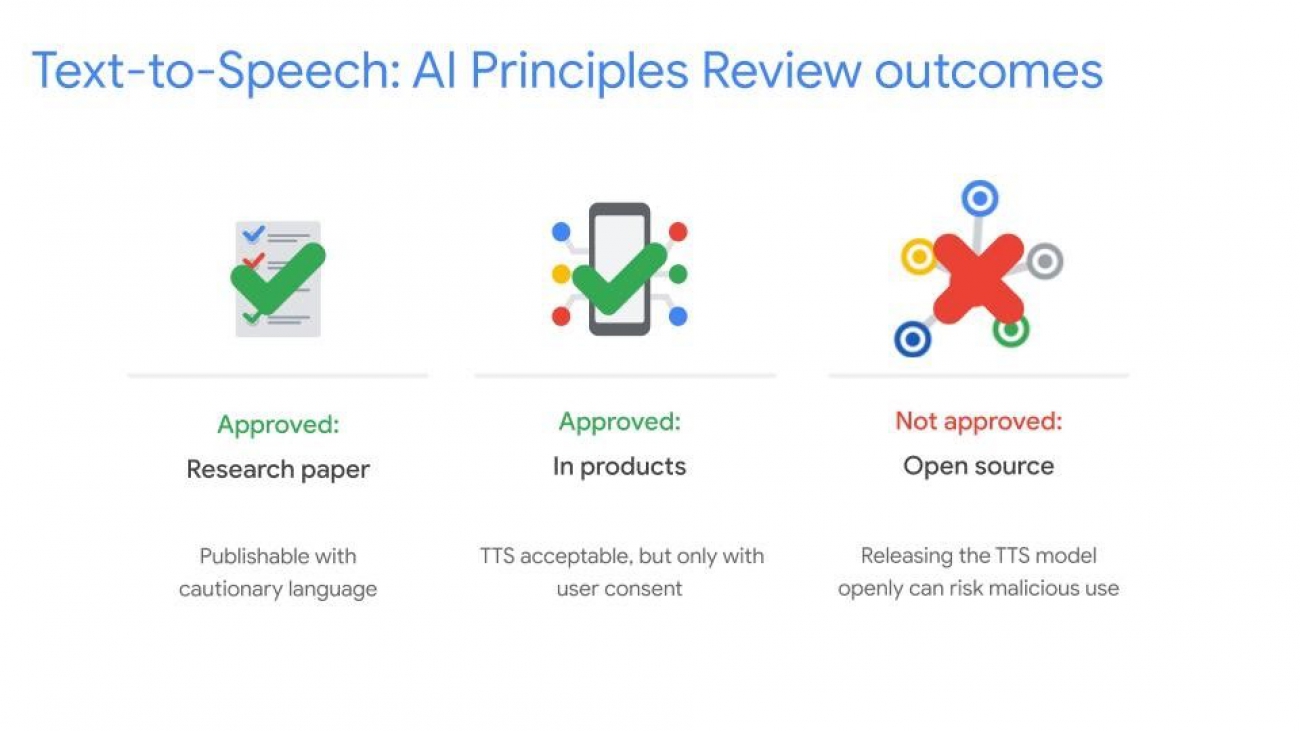
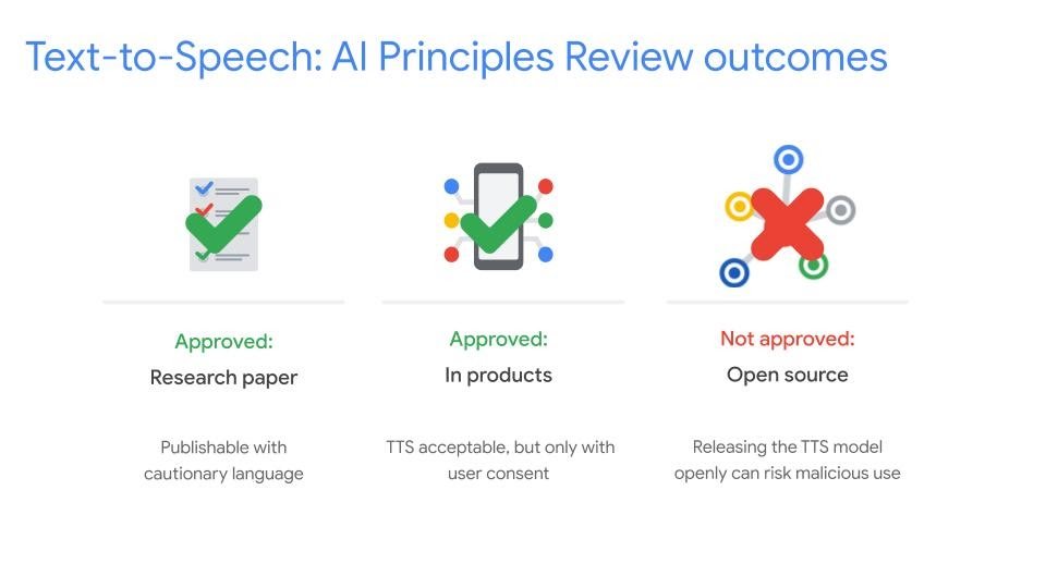
Convolutional neural networks (CNNs) achieve state-of-the-art results in tasks such as image classification and object detection. They are used in many diverse applications, such as in autonomous driving to detect traffic signs and objects on the street, in healthcare to more accurately classify anomalies in image-based data, and in retail for inventory management.

However, CNNs act as a black box, which can be problematic in applications where it’s critical to understand how predictions are made. Also, after the model is deployed, the data used for inference may follow a very different distribution compared to the data from which the model was trained. This phenomenon is commonly referred to as data drift, and can lead to incorrect model predictions. In this context, understanding and being able to explain what leads to an incorrect model prediction is important.

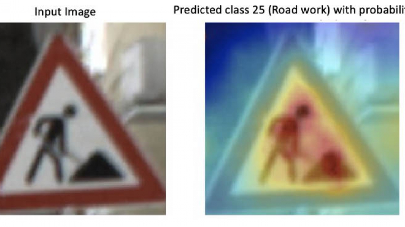
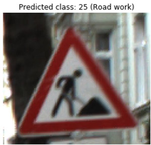
Techniques such as class activation maps and saliency maps allow you to visualize how a CNN model makes a decision. These maps rendered as heat maps reveal the parts of an image that are critical in the prediction. The following example images are from the German Traffic Sign dataset: the image on the left is the input into a fine-tuned ResNet model, which predicts the image class 25 (Road work). The right image shows the input image overlaid with a heat map, where red indicates the most relevant and blue the least relevant pixels for predicting the class 25.

Visualizing the decisions of a CNN is especially helpful if a model makes an incorrect prediction and it’s not clear why. It also helps you figure out whether the training datasets require more representative samples or if there is bias in the dataset. For example, if you have an object detection model to find obstacles in road traffic and the training dataset only contains samples taken during summer, it likely won’t perform well during winter because it hasn’t learned that objects could be covered in snow.

In this post, we deploy a model for traffic sign classification and set up Amazon SageMaker Model Monitor to automatically detect unexpected model behavior, such as consistently low prediction scores or overprediction of certain image classes. When Model Monitor detects an issue, we use Amazon SageMaker Debugger to obtain visual explanations of the deployed model. You can do this by updating the endpoint to emit tensors during inference and using those tensors to compute saliency maps. To reproduce the different steps and results listed in this post, clone the repository amazon-sagemaker-analyze-model-predictions into your Amazon SageMaker notebook instance or from within your Amazon SageMaker Studio and run the notebook.

Defining a SageMaker model

This post uses a ResNet18 model trained to distinguish between 43 categories of traffic signs using the German Traffic Sign dataset [2]. When given an input image, the model outputs probabilities for the different image classes. Each class corresponds to a different traffic sign category. We have fine-tuned the model and uploaded its weights to the GitHub repo.

Before you can deploy the model to Amazon SageMaker, you need to archive and upload its weights to Amazon Simple Storage Service (Amazon S3). Enter the following code in a Jupyter notebook cell:

sagemaker_session.upload_data(path='model.tar.gz', key_prefix='model')

You use Amazon SageMaker hosting services to set up a persistent endpoint to get predictions from the model. Therefore, you need to define a PyTorch model object that takes the Amazon S3 path of the model archive. Define an entry_point file pretrained_model.py that implements the model_fn and transform_fn functions. You use those functions during hosting to make sure that the model is correctly loaded inside the inference container and that incoming requests are properly processed. See the following code:

from sagemaker.pytorch.model import PyTorchModel

model = PyTorchModel(model_data = 's3://' + sagemaker_session.default_bucket() + '/model/model.tar.gz',
                     role = role,
                     framework_version = '1.5.0',
                     source_dir='entry_point',
                     entry_point = 'pretrained_model.py',
                     py_version='py3')

Setting up Model Monitor and deploying the model

Model Monitor automatically monitors machine learning models in production and alerts you when it detects data quality issues. In this solution, you capture the inputs and outputs of the endpoint and create a monitoring schedule to let Model Monitor inspect the collected data and model predictions. The DataCaptureConfig API specifies the fraction of inputs and outputs that Model Monitor stores in a destination Amazon S3 bucket. In the following example, the sampling percentage is set to 50%:

from sagemaker.model_monitor import DataCaptureConfig

data_capture_config = DataCaptureConfig(
    enable_capture=True,
    sampling_percentage=50,
    destination_s3_uri='s3://' + sagemaker_session.default_bucket() + '/endpoint/data_capture'
)

To deploy the endpoint to an ml.m5.xlarge instance, enter the following code:

predictor = model.deploy(initial_instance_count=1,
                        instance_type='ml.m5.xlarge',
                        data_capture_config=data_capture_config)
                        
endpoint_name = predictor.endpoint 

Running inference with test images

Now you can invoke the endpoint with a payload that contains serialized input images. The endpoint calls the transform_fn function to preprocess the data before performing model inference. The endpoint returns the predicted classes of the image stream as a list of integers, encoded in a JSON string. See the following code:

#invoke payload
response = runtime.invoke_endpoint(EndpointName=endpoint_name, Body=payload)
response_body = response['Body']

#get results
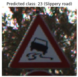
result = json.loads(response_body.read().decode())

You can now visualize some test images and their predicted class. In the following visualization, the traffic sign images are what was sent to the endpoint for prediction, and the top labels are the corresponding predictions received from the endpoint. The following image shows that the endpoint correctly predicted class 23 (Slippery road).

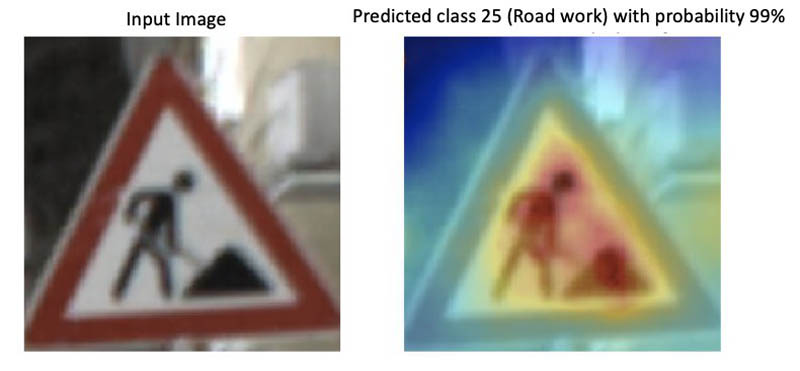
The following image shows that the endpoint correctly predicted class 25 (Road work).

Creating a Model Monitor schedule

Next, we demonstrate how to set up a monitoring schedule using Model Monitor. Model Monitor provides a built-in container to create a baseline that calculates constraints and statistics such as mean, quantiles, and standard deviation. You can then launch a monitoring schedule that periodically kicks off a processing job to inspect collected data, compare the data against the given constraints, and generate a violations report.

For this use case, you create a custom container that performs a simple model sanity check: it runs an evaluation script that counts the predicted image classes. If the model predicts a particular street sign more often than other classes, or if confidence scores are consistently low, it indicates an issue.

For example, with a given input image, the model returns a list of predicted classes ranked based on the confidence score. If the top three predictions correspond to unrelated classes, each with confidence score below 50% (for example, Stop sign as the first prediction, Turn left as the second, and Speed limit 180 km/h as the third), you may not want to trust those predictions.

For more information about building your custom container and uploading it to Amazon Elastic Container Registry (Amazon ECR) see the notebook. The following code creates a Model Monitor object where you indicate the location of the Docker image in Amazon ECR and the environment variables that the evaluation script requires. The container’s entry point file is the evaluation script.

monitor = ModelMonitor(
    role=role,
    image_uri='%s.dkr.ecr.us-west-2.amazonaws.com/sagemaker-processing-container:latest' %my_account_id,
    instance_count=1,
    instance_type='ml.m5.xlarge',
    env={'THRESHOLD':'0.5'}
)

Next, define and attach a Model Monitor schedule to the endpoint. It runs your custom container on an hourly basis. See the following code:

from sagemaker.model_monitor import CronExpressionGenerator
from sagemaker.processing import ProcessingInput, ProcessingOutput

destination = 's3://' + sagemaker_session.default_bucket() + '/endpoint/monitoring_schedule'
processing_output = ProcessingOutput(output_name='model_outputs', source='/opt/ml/processing/outputs', destination=destination)
output = MonitoringOutput(source=processing_output.source, destination=processing_output.destination)

monitor.create_monitoring_schedule(
    output=output,
    endpoint_input=predictor.endpoint,
    schedule_cron_expression=CronExpressionGenerator.hourly()
)

As previously described, the script evaluation.py performs a simple model sanity check: it counts the model predictions. Model Monitor saves model inputs and outputs as JSON-line formatted files in Amazon S3. They are downloaded in the processing container under /opt/ml/processing/input. You can then load the predictions via ['captureData']['endpointOutput']['data']. See the following code:

for file in files:
    content = open(file).read()
   for entry in content.split('n'):
        prediction = json.loads(entry)['captureData']['endpointOutput']['data']

You can track the status of the processing job in CloudWatch and also in SageMaker Studio. In the following screenshot, SageMaker Studio shows that no issues were found.

Capturing unexpected model behavior

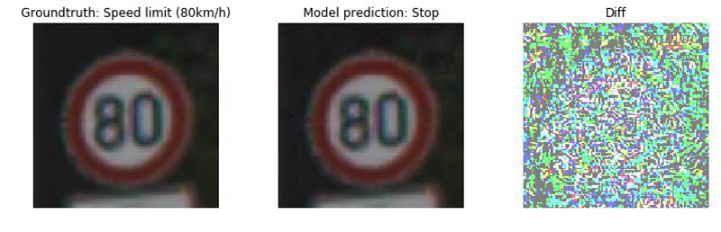
Now that the schedule is defined, you’re ready to monitor the model in real time. To verify that the setup can capture unexpected behavior, you enforce false predictions. To achieve this, we use AdvBox Toolkit [3], which introduces perturbations at the pixel level such the model doesn’t recognize correct classes any longer. Such perturbations are also known as adversarial attacks, and are typically invisible to human observers. We converted some test images that are now predicted as Stop signs. In the following set of images, the image is the original, the middle is the adversarial image, and the right is the difference between both. The original and adversarial images look similar, but the adversarial isn’t classified correctly.

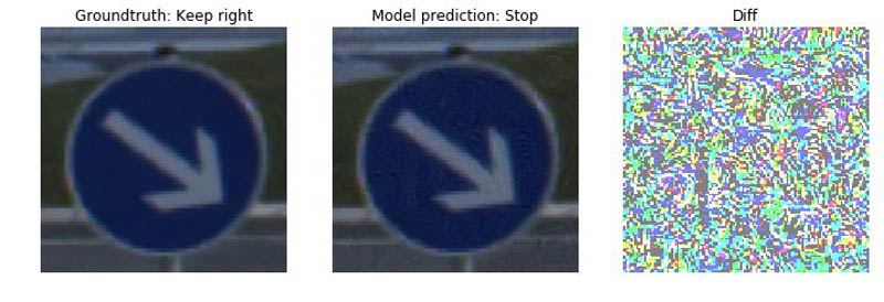
The following set of images shows another incorrectly classified sign.

When Model Monitor schedules the next processing job, it analyzes the predictions that were captured and stored in Amazon S3. The job counts the predicted image classes; if one class is predicted more than 50% of the time, it raises an issue. Because we sent adversarial images to the endpoint, you can now see an abnormal count for the image class 14 (Stop). You can track the status of the processing job in SageMaker Studio. In the following screenshot, SageMaker Studio shows that the last scheduled job found an issue.

You can get further details from the Amazon CloudWatch logs: the processing job prints a dictionary where the key is one of 43 image classes and the value is the count. For instance, in the following output, the endpoint predicted the image class 9 (No passing) twice and an abnormal count for class 14 (Stop). It predicted this class 322 times out of 400 total predictions, which is higher than the 50% threshold. The values of the dictionary are also stored as CloudWatch metrics, so you can create graphs of the metric data using the CloudWatch console.

Warning: Class 14 ('Stop sign') predicted more than 80 % of the time which is above the threshold
Predicted classes {9: 2, 19: 2, 25: 1, 14: 322, 13: 5, 5: 1, 8: 10, 18: 1, 31: 4, 26: 8, 33: 4, 36: 4, 29: 20, 12: 8, 22: 4, 6: 4}

Now that the processing job found an issue, it’s time to get further insights. When looking at the preceding test images, there’s no significant difference between the original and the adversarial images. To get a better understanding of what the model saw, you can use the technique described in the paper Full-Gradient Representation for Neural Network Visualization [1], which uses importance scores of input features and intermediate feature maps. In the following section, we show how to configure Debugger to easily retrieve these variables as tensors without having to modify the model itself. We also go into more detail about how to use those tensors to compute saliency maps.

Creating a Debugger hook configuration

To retrieve the tensors, you need to update the pretrained model Python script, pretrained_model.py, which you ran at the very beginning to set up an Amazon SageMaker PyTorch model. We created a Debugger hook configuration in model_fn, and the hook takes a customized string into the parameter, include_regex, which passes regular expressions of the full or partial names of tensors that we want to collect. In the following section, we show in detail how to compute saliency maps. The computation requires bias and gradients from intermediate layers such as BatchNorm and downsampling layers and the model inputs. To obtain the tensors, indicate the following regular expression:

'.*bn|.*bias|.*downsample|.*ResNet_input|.*image'

Store the tensors in your Amazon SageMaker default bucket. See the following code:

def model_fn(model_dir):
    
    #load model
    model = resnet.resnet18()
    model.load_state_dict(torch.load(model_dir))
    model.eval()
    
    #hook configuration
    save_config = smd.SaveConfig(mode_save_configs={
        smd.modes.PREDICT: smd.SaveConfigMode(save_interval=1)
    })
    
    hook = Hook("s3://" + sagemaker_session.default_bucket() + "tensors", 
                    save_config=save_config, 
                    include_regex='.*bn|.*bias|.*downsample|.*ResNet_input|.*image' )
    
    #register hook
    hook.register_module(model) 
    
    #set mode
    hook.set_mode(modes.PREDICT)
    
    return model 

Create a new PyTorch model using the new entry point script pretrained_model_with_debugger_hook.py:

model = PyTorchModel(model_data = 's3://' + sagemaker_session.default_bucket() + '/model/model.tar.gz',
                        role = role,
                        framework_version = '1.3.1',
                        source_dir='code',
                        entry_point = 'pretrained_model_with_debugger_hook.py',
                        py_version='py3')

Update the existing endpoint using the new PyTorch model object that took the modified model script with the Debugger hook:

predictor = model.deploy(
        instance_type = 'ml.m5.xlarge',
        initial_instance_count=1,
        endpoint_name=endpoint_name,
        data_capture_config=data_capture_config,
        update_endpoint=True)

Now, whenever an inference request is made, the endpoint records tensors and uploads them to Amazon S3. You can now compute saliency maps to get visual explanations from the model.

Analyzing incorrect predictions with Debugger

A classification model typically outputs an array of probabilities between 0 and 1, where each entry corresponds to a label in the dataset. For example, in the case of MNIST (10 classes), a model may produce the following prediction for the input image with digit 8: [0.08, 0, 0, 0, 0, 0, 0.12, 0, 0.5, 0.3], meaning the image is predicted to be 0 with 8% probability, 6 with 12% probability, 8 with 50% probability, and 9 with 30% probability. To generate a saliency map, you take the class with the highest probability (for this use case, class 8) and map the score back to previous layers in the network to identify the important neurons for this prediction. CNNs consist of many layers, so an importance score for each intermediate value that shows how each value contributed to the prediction is calculated.

You can use the gradients of the predicted outcome from the model with respect to the input to determine the importance scores. The gradients show how much the output changes when inputs are changing. To record them, register a backward hook on the layer outputs and trigger a backward call during inference. We have configured the Debugger hook to capture the relevant tensors.

After you update the endpoint and perform some inference requests, you can create a trial object, which enables you to access, query, and filter the data that Debugger saved. See the following code:

from smdebug.trials import create_trial

trial = create_trial('s3://' + sagemaker_session.default_bucket() + '/endpoint/tensors')

With Debugger, you can access the data via trial.tensor().value(). For example, to get the bias tensor of the first BatchNorm layer of the first inference request, enter the following code:

trial.tensor('ResNet_bn1.bias').value(step_num=0, mode=modes.PREDICT).

The function trial.steps(mode=modes.PREDICT) returns the number of steps available, which corresponds to the number of inference requests recorded.

In the following steps, you compute saliency maps based on the FullGrad method, which aggregates input gradients and feature-level bias gradients.

Computing implicit biases

In the FullGrad method, the BatchNorm layers of ResNet18 introduce an implicit bias. You can compute the implicit bias by retrieving the running mean, variance, and the weights of the layer. See the following code:

weight = trial.tensor(weight_name).value(step_num=step, mode=modes.PREDICT)
running_var = trial.tensor(running_var_name).value(step_num=step, mode=modes.PREDICT)
running_mean = trial.tensor(running_mean_name).value(step_num=step, mode=modes.PREDICT)
implicit_bias = - running_mean / np.sqrt(running_var) * weight

Multiplying gradients and biases

Bias is the sum of explicit and implicit bias. You can retrieve the gradients of the output with respect to the feature maps and compute the product of bias and gradients. See the following code:

gradient = trial.tensor(gradient_name).value(step_num=step, mode=modes.PREDICT)
bias = trial.tensor(bias_name).value(step_num=step, mode=modes.PREDICT) 
bias = bias + implicit_bias
bias_gradient = normalize(np.abs(bias * gradient))

Interpolating and aggregating

Intermediate layers typically don’t have the same dimensions as the input image, so you need to interpolate them. You do this for all bias gradients and aggregate the results. The overall sum is the saliency map that you overlay as the heat map on the original input image. See the following code:

for channel in range(bias_gradient.shape[1]):
    interpolated = scipy.ndimage.zoom(bias_gradient[0,channel,:,:], image_size/bias_gradient.shape[2], order=1)
   saliency_map += interpolated 

Results

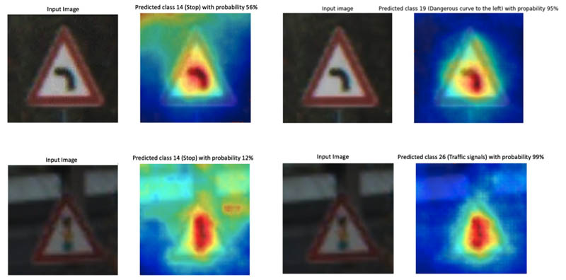
In this section, we include some examples of adversarial images that the model classified as stop signs. The images on the right show the model input overlaid with the saliency map. Red indicates the part that had the largest influence in the model prediction, and may indicate the location of pixel perturbations. You can see, for instance, that relevant object features are no longer taken into account by the model, and in most cases the confidence scores are low.

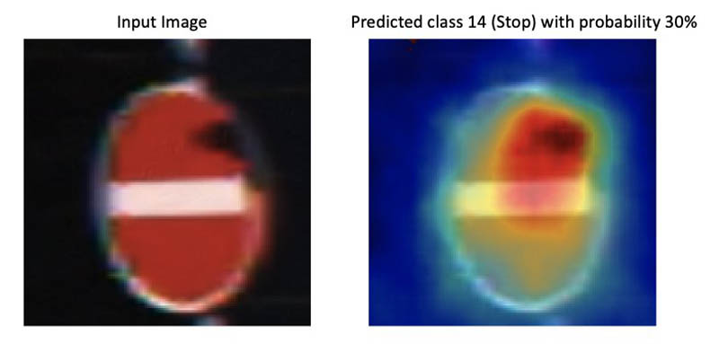
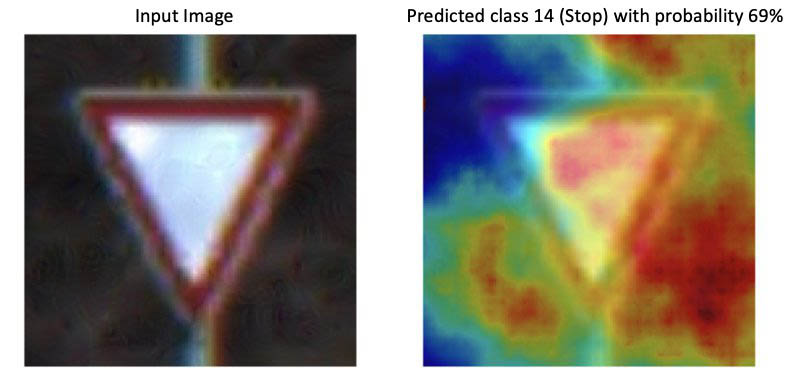
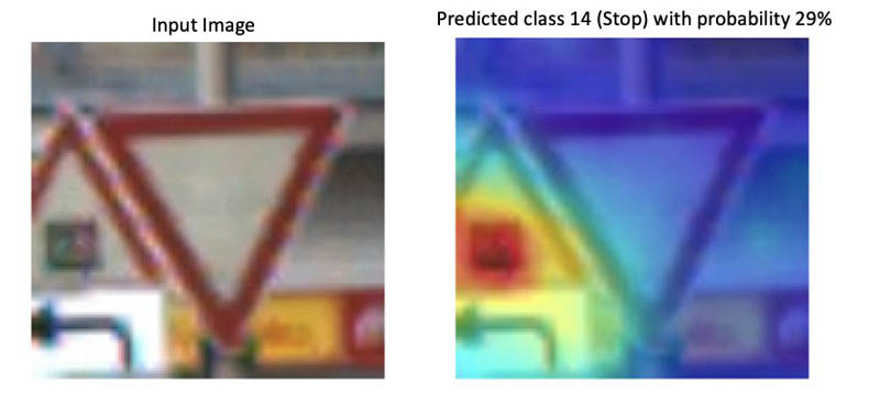
For comparison, we also perform inference with original (non-adversarial) images. In the following image sets, the image on the left is the adversarial image and the corresponding saliency map for the predicted image class Stop. The right images show the original input image (non-adversarial) and the corresponding saliency map for the predicted image class (which corresponds to the ground-truth label). In the case of non-adversarial images, the model only focuses on relevant object features and therefore predicts the correct image class with a high probability. In the case of adversarial images, the model takes many other features outside of the relevant object into account, which is caused by the random pixel perturbations.

Summary

This post demonstrated how to use Amazon SageMaker Model Monitor and Amazon SageMaker Debugger to automatically detect unexpected model behavior and to get visual explanations from a CNN. For more information, see the GitHub repo.

References


About the Authors

Nathalie Rauschmayr is an Applied Scientist at AWS, where she helps customers develop deep learning applications.


Vikas Kumar is Senior Software Engineer for AWS Deep Learning, focusing on building scalable deep learning systems and providing insights into deep learning models. Prior to this Vikas has worked on building distributed databases and service discovery software. In his spare time he enjoys reading and music.


Satadal Bhattacharjee is Principal Product Manager at AWS AI. He leads the machine learning engine PM team on projects such as SageMaker and optimizes machine learning frameworks such as TensorFlow, PyTorch, and MXNet.


Read More

Announcing the launch of Amazon Comprehend custom entity recognition real-time endpoints

Announcing the launch of Amazon Comprehend custom entity recognition real-time endpoints

Amazon Comprehend is a natural language processing (NLP) service that can extract key phrases, places, names, organizations, events, sentiment from unstructured text, and more (for more information, see Detect Entities). But what if you want to add entity types unique to your business, like proprietary part codes or industry-specific terms? In November 2018, Amazon Comprehend added the ability to extend the default entity types to detect custom entities.

Until now, inference with a custom entity recognition model was an asynchronous operation.

In this post, we cover how to build an Amazon Comprehend custom entity recognition model and set up an Amazon Comprehend Custom Entity Recognition real time endpoint for synchronous inference. The following diagram illustrates this architecture.

Solution overview

Amazon Comprehend Custom helps you meet your specific needs without requiring machine learning (ML) knowledge. Amazon Comprehend Custom uses automatic ML (AutoML) to build customized NLP models on your behalf, using data you already have.

For example, if you’re looking at chat messages or IT tickets, you might want to know if they’re related to an AWS offering. You need to build a custom entity recognizer that can identify a word or a group of words as a SERVICE or VERSION entity from the input messages.

In this post, we walk you through the following steps to implement a solution for this use case:

  1. Create a custom entity recognizer trained on annotated labels to identify custom entities such as SERVICE or VERSION.
  2. Create a real-time analysis Amazon Comprehend custom entity recognizer endpoint to identify the chat messages to detect a SERVICE or VERSION entity.
  3. Calculate the inference capacity and pricing for your endpoint.

We provide a sample dataset aws-service-offerings.txt. The following screenshot shows example entries from the dataset.

You can provide labels for training a custom entity recognizer in two different ways: entity lists and annotations. We recommend annotations over entity lists because the increased context of the annotations can often improve your metrics. For more information, see Improving Custom Entity Recognizer Performance. We preprocessed the input dataset to generate training data and annotations required for training the custom entity recognizer.

You can download these files below:

After you download these files, upload them to an Amazon Simple Storage Service (Amazon S3) bucket in your account for reference during training. For more information about uploading files, see How do I upload files and folders to an S3 bucket?
For more information about creating annotations or labels for your custom dataset, see Developing NER models with Amazon SageMaker Ground Truth and Amazon Comprehend.

Creating a custom entity recognizer

To create your recognizer, complete the following steps:

  1. On the Amazon Comprehend console, create a custom entity recognizer.
  2. Choose Train recognizer.
  3. For Recognizer name, enter aws-offering-recognizer.
  4. For Custom entity type, enter SERVICE.
  5. Choose Add type.
  6. Enter a second Custom entity type called VERSION.
  7. For Training type, select Using annotations and training docs.
  8. For Annotations location on S3, enter the path for annotations.csv in your S3 bucket.
  9. For Training documents location on S3, enter the path for train.csv in your S3 bucket.
  10. For IAM role, select Create an IAM role.
  11. For Permissions to access, choose Input and output (if specified) S3 bucket.
  12. For Name suffix, enter ComprehendCustomEntity.
  13. Choose Train.

For our dataset, training should take approximately 10 minutes.

When the recognizer training is complete, you can review the training metrics in the Recognizer details section.

Scroll down to see the individual training performance.

For more information about understanding these metrics and improving recognizer performance, see Custom Entity Recognizer Metrics.

When training is complete, you can use the recognizer to detect custom entities in your documents. You can quickly analyze single documents up to 5 KB in real time, or analyze a large set of documents with an asynchronous job (using Amazon Comprehend batch processing).

Creating a custom entity endpoint

Creating your endpoint is a two-step process: building an endpoint and then using it by running a real-time analysis.

Building the endpoint

To create your endpoint, complete the following steps:

  1. On the Amazon Comprehend console, choose Customization.
  2. Choose Custom entity recognition.
  3. From the Recognizers list, choose the name of the custom model for which you want to create the endpoint and follow the link. The endpoints list on the custom model details page is displayed. You can also see previously created endpoints and the models they’re associated with.
  4. Select your model.
  5. From the Actions drop-down menu, choose Create endpoint.
  6. For Endpoint name, enter DetectEntityServiceOrVersion.

The name must be unique within the AWS Region and account. Endpoint names have to be unique even across recognizers.

  1. For Inference units, enter the number of inference units (IUs) to assign to the endpoint.

We discuss how to determine how many IUs you need later in this post.

  1. As an optional step, under Tags, enter a key-value pair as a tag.
  2. Choose Create endpoint.

The Endpoints list is displayed, with the new endpoint showing as Creating. When it shows as Ready, you can use the endpoint for real-time analysis.

Running real-time analysis

After you create the endpoint, you can run real-time analysis using your custom model.

  1. For Analysis type, select Custom.
  2. For Endpoint, choose the endpoint you created.
  3. For Input text, enter the following:
    AWS Deep Learning AMI (Amazon Linux 2) Version 220 The AWS Deep Learning AMIs are prebuilt with CUDA 8 and several deep learning frameworks.The DLAMI uses the Anaconda Platform with both Python2 and Python3 to easily switch between frameworks.
    

  4. Choose Analyze.

You get insights as in the following screenshot, with entities recognized as either SERVICE or VERSION and their confidence score.

You can experiment with different input text combinations to compare and contrast the results.

Determining the number of IUs you need

The number of IUs you need depends on the number of characters you send in your request and the throughput you need from Amazon Comprehend. In this section, we discuss two different use cases with different costs.

In all cases, endpoints are billed in 1-second increments, with a minimum of 60 seconds. Charges continue to incur from the time you provision your endpoint until it’s deleted, even if no documents are analyzed. For more information, see Amazon Comprehend Pricing.

Use case 1

In this use case, you receive 10 messages/feeds every minute, and each message is comprised of 360 characters that you need to recognize entities for. This equates to the following:

  • 60 characters per second (360 characters x 10 messages ÷ 60 seconds)
  • An endpoint with 1 IU provides a throughput of 100 characters per second

You need to provision an endpoint with 1 IU. Your recognition model has the following pricing details:

  • The price for 1 IU is $0.0005 per second
  • You incur costs from the time you provision your endpoint until it’s deleted, regardless of how many inference calls are made
  • If you’re running your real-time endpoint for 12 hours a day, this equates to a total cost of $21.60 ($0.0005 x 3,600 seconds x 12 hours) for inference
  • The model training and model management costs are the same as for asynchronous entity recognition at $3.00 and $0.50, respectively

The total cost of an hour of model training, a month of model management, and inference using a real-time entity recognition endpoint for 12 hours a day is $25.10 per day.

Use case 2

In this second use case, your requirement increased to run inference for 50 messages/feeds every minute, and each message contains 600 characters that you need to recognize entities for. This equates to the following:

  • 500 characters per second (600 characters x 50 messages ÷ 60 seconds)
  • An endpoint with 1 IU provides a throughput of 100 characters per second.

You need to provision an endpoint with 5 IU. Your model has the following pricing details:

  • The price for 1 IU the $0.0005 per second
  • You incur costs from the time you provision your endpoint until it’s deleted, regardless of how many inference calls are made
  • If you’re running your real-time endpoint for 12 hours a day, this equates to a total cost of $108 (5 x $0.0005 x 3,600 seconds x 12 hours) for inference
  • The model training and model management costs are the same as for asynchronous entity recognition at $3.00 and $0.50, respectively

The total cost of an hour of model training, a month of model management, and inference using a real-time entity recognition endpoint with a throughput of 5 IUs for 12 hours a day is $111.50.

Cleaning up

To avoid incurring future charges, stop or delete resources (the endpoint, recognizer, and any artifacts in Amazon S3) when not in use.

To delete your endpoint, on the Amazon Comprehend console, choose the entity recognizer you created. In the Endpoints section, choose Delete.

To delete your recognizer, in the Recognizer details section, choose Delete.

For instructions on deleting your S3 bucket, see Deleting or emptying a bucket.

Conclusion

This post demonstrated how easy it is to set up an endpoint for real-time text analysis to detect custom entities that you trained your Amazon Comprehend custom entity recognizer on. Custom entity recognition extends the capability of Amazon Comprehend by enabling you to identify new entity types not supported as one of the preset generic entity types. With Amazon Comprehend custom entity endpoints, you can now easily derive real-time insights on your custom entity detection models, providing a low latency experience for your applications. We’re interested to hear how you would like to apply this new feature to your use cases. Please share your thoughts and questions in the comments section.


About the Authors

Mona Mona is an AI/ML Specialist Solutions Architect based out of Arlington, VA. She works with the World Wide Public Sector team and helps customers adopt machine learning on a large scale. She is passionate about NLP and ML explainability areas in AI/ML.


Prem Ranga is an Enterprise Solutions Architect based out of Houston, Texas. He is part of the Machine Learning Technical Field Community and loves working with customers on their ML and AI journey. Prem is passionate about robotics, is an autonomous vehicles researcher, and also built the Alexa-controlled Beer Pours in Houston and other locations.


Read More

Optimizing I/O for GPU performance tuning of deep learning training in Amazon SageMaker

Optimizing I/O for GPU performance tuning of deep learning training in Amazon SageMaker

GPUs can significantly speed up deep learning training, and have the potential to reduce training time from weeks to just hours. However, to fully benefit from the use of GPUs, you should consider the following aspects:

  • Optimizing code to make sure that underlying hardware is fully utilized
  • Using the latest high performant libraries and GPU drivers
  • Optimizing I/O and network operations to make sure that the data is fed to the GPU at the rate that matches its computations
  • Optimizing communication between GPUs during multi-GPU or distributed training

Amazon SageMaker is a fully managed service that enables developers and data scientists to quickly and easily build, train, and deploy machine learning (ML) models at any scale. In this post, we focus on general techniques for improving I/O to optimize GPU performance when training on Amazon SageMaker, regardless of the underlying infrastructure or deep learning framework. You can typically see performance improvements up to 10-fold in overall GPU training by just optimizing I/O processing routines.

The basics

A single GPU can perform tera floating point operations per second (TFLOPS), which allows them to perform operations 10–1,000 times faster than CPUs. For GPUs to perform these operations, the data must be available in the GPU memory. The faster you load data into GPU, the quicker it can perform its operation. The challenge is to optimize I/O or the network operations in such a way that the GPU never has to wait for data to perform its computations.

The following diagram illustrates the architecture of optimizing I/O.

The general steps usually involved in getting the data into the GPU memory are the following:

  • Network operations – Download the data from Amazon Simple Storage Service (Amazon S3).
  • Disk I/O – Read data from local disk into CPU memory. Local disk refers to an instance store, where storage is located on disks that are physically attached to the host computer. Amazon Elastic Block Store (Amazon EBS) volumes aren’t local resources, and involve network operations.
  • Data preprocessing – The CPU generally handles any data preprocessing such as conversion or resizing. These operations might include converting images or text to tensors or resizing images.
  • Data transfer into GPU memory – Copy the processed data from the CPU memory into the GPU memory.

The following sections look at optimizing these steps.

Optimizing data download over the network

In this section, we look at tips to optimize data transfer via network operations, e.g. downloading data from Amazon S3, use of file systems such as Amazon EBS & Amazon Elastic File System (Amazon EFS).

Optimizing file sizes

You can store large amounts of data in Amazon S3 at low cost. This includes data from application databases extracted through an ETL process into a JSON or CSV format or image files. One of the first steps that Amazon SageMaker does is download the files from Amazon S3, which is the default input mode called File mode.

Downloading or uploading very small files, even in parallel, is slower than larger files totaling up to the same size. For instance, if you have 2,000,000 files, where each file is 5 KB (total size = 10 GB = 2,000,000 X 5 * 1024), downloading these many tiny files can take a few hours, compared to a few minutes when downloading 2,000 files each 5 MB in size (total size = 10 GB = 2,000 X 5 * 1024 * 1024 ), even though the total download size is the same.

One of the primary reasons for this is the read/write block size. Assume that the total volume and the number of threads used for transfer is roughly the same for the large and the small files. If the transfer block size is 128 KB and the file size is 2 KB, instead of transferring 128 KB at one time, you only transfer 2 KB.

On the other hand, if the files are too large, you can’t take advantage of parallel processing to upload or download data to make it faster unless you use options such as Amazon S3 range gets to download different blocks in parallel.

Formats like MXNet RecordIO and TFRecord allow you to compress and densely pack multiple image files into a single file to avoid this trade-off. For instance, MXNet RecordIO for images recommends that images are reduced in size so you can fit at least a batch of images into CPU/GPU memory and multiple images are densely packed into a single file, so I/O operations on a tiny file don’t become a bottleneck.

As a general rule, the optimal file size ranges from 1–128 MB.

Amazon SageMaker ShardedByS3Key Amazon S3 data distribution for large datasets

During distributed training, you can also shard very large datasets across various instances. You can achieve this in an Amazon SageMaker training job by setting the parameter S3DataDistributionType to ShardedByS3Key. In this mode, if the Amazon S3 input dataset has total M objects and the training job has N instances, each instance handles M/N objects. For more information, see S3DataSource. For this use case, model training on each machine uses only the subset of training data.

Amazon SageMaker Pipe mode for large datasets

Compared to SageMaker File mode, Pipe mode allows large data to be streamed directly to your training instances from Amazon S3 instead of downloading to disk first. Pipe mode allows your code to access the data without having to wait for the entire download. Because data is never downloaded to disk and only a relatively smaller footprint is maintained in memory, data is continuously downloaded from Amazon S3 throughout each epoch. This makes it a great fit for working with very large datasets that can’t fit into the CPU memory. To take advantage of the partial raw bytes as they become available when streamed, you need your code to decode the bytes depending on the record format (such as CSV) and find the end of record to convert the partial bytes into a logical record. Amazon SageMaker TensorFlow provides built-in Pipe mode dataset readers for common formats such as text files and TFRecord. For more information, see Amazon SageMaker Adds Batch Transform Feature and Pipe Input Mode for TensorFlow Containers. If you use frameworks or libraries that don’t have built-in data readers, you could use ML-IO libraries or write your own data readers to make use of Pipe mode.

Another consequence of Pipe mode streaming is that to shuffle the data, you should use ShuffleConfig to shuffle the results of the Amazon S3 key prefix matches or lines in a manifest file and augmented manifest file. If you have one large file, you can’t rely on Amazon SageMaker to do the shuffling; you have to prefetch “N” number of batches and write your own code to shuffle depending on your ML framework.

If you can fit the entire dataset into CPU memory, File mode can be more efficient than Pipe mode. This is because if you can easily fit the entire dataset into the CPU memory, with File mode, you need to download the entire dataset into disk one time, load the entire dataset into memory one time, and repeatedly read from memory across all epochs. Reading from memory is typically much faster than network I/O, which allows you to achieve better performance.

The following section discusses how to deal with very large datasets.

Amazon FSx for Lustre or Amazon EFS for large datasets

For very large datasets, you can reduce Amazon S3 download times by using a distributed file system.

You can reduce startup times using Amazon FSx for Lustre on Amazon SageMaker while maintaining the data in Amazon S3. For more information, see Speed up training on Amazon SageMaker using Amazon FSx for Lustre and Amazon EFS file systems.

The first time you run a training job, FSx for Lustre automatically copies data from Amazon S3 and makes it available to Amazon SageMaker. Additionally, you can use the same FSx for Lustre file system for subsequent iterations of training jobs on Amazon SageMaker, which prevents repeated downloads of common Amazon S3 objects. Because of this, FSx for Lustre has the most benefit for training jobs that have training sets in Amazon S3 and in workflows where training jobs must be run several times using different training algorithms or parameters to see which gives the best result.

If you already have your training data on Amazon Elastic File System (Amazon EFS), you can also use Amazon EFS with Amazon SageMaker. For more information, see Speed up training on Amazon SageMaker using Amazon FSx for Lustre and Amazon EFS file systems.

One thing to consider while using this option is file size. If the file sizes are too small, the I/O performance is likely to be slower due to factors such as transfer block size.

Amazon SageMaker instances with local NVMe-based SSD storage

Some of the Amazon SageMaker GPU instances, such as the ml.p3dn.24xlarge and ml.g4dn, provide local NVMe-based SSD storage instead of EBS volumes. For instance, the ml.p3dn.24xlarge instances have 1.8 TB of local NVMe-based SSD storage. The use of local NVMe-based SSD storage means that after training data is downloaded from Amazon S3 to a local disk storage, the disk I/0 is much faster than reading from network resources such as EBS volumes or Amazon S3. This allows you to achieve faster training times when the training data size can fit into the local NVMe-based storage.

Optimizing data loading and preprocessing

In the preceding section, we described how to download data from sources like Amazon S3 efficiently. In this section, we discuss how to increase parallelism and make commonly used functions as lean as possible to make data loading more efficient.

Multiple workers for loading and processing data

TensorFlow, MXNet Gluon, and PyTorch provide data loader libraries for loading data in parallel. In the following PyTorch example, increasing the number of workers allows more workers to process items in parallel. As a general rule, you may scale up from a single worker to approximately one less than the number of CPUs. Generally, each worker represents one process and uses Python multiprocessing, although the implementation details can vary from framework to framework. The use of multiprocessing sidesteps the Python Global Interpreter Lock (GIL) to fully use all the CPUs in parallel, but it also means that memory utilization increases proportionally to the number of workers because each process has its own copy of the objects in memory. You might see out of memory exceptions as you start to increase the number of workers, in which case you should use an instance that has more CPU memory where applicable.

To understand the effect of using the workers, we present the following example dataset. In this dataset, the __get_item__ operation sleeps for 1 second, to emulate some latency in reading the next record:

class MockDatasetSleep(Dataset):
    """
    Simple mock dataset to understand the use of workers
    """

    def __init__(self, num_cols, max_records=32):
        super(MockDatasetSleep).__init__()
        self.max_records = max_records
        self.num_cols = num_cols

        # Initialising mock x and y
        self.x = np.random.uniform(size=self.num_cols)
        self.y = np.random.normal()
        
        print("Initialised")


    def __len__(self):
        return self.max_records

    def __getitem__(self, idx):
        curtime = datetime.datetime.now()

        # Emulate a slow operation
        sleep_seconds = 1

        time.sleep(sleep_seconds)
        print("{}: retrieving item {}".format(curtime, idx))

        return self.x, self.y

As an example, create a data loader instance with only a single worker:

# One worker
num_workers = 1
torch.utils.data.DataLoader(MockDatasetSleep(), batch_size=batch_size, shuffle=True, num_workers=num_workers)

When you use a single worker, you see items retrieved one by one, with a 1-second delay to retrieve each item:

15:39:58.833644: retrieving item 0
15:39:59.834420: retrieving item 6
15:40:00.834861: retrieving item 8
15:40:01.835350: retrieving item 5

If you increase the number of workers to 3 workers on an instance, that has at least 4 CPUs to ensure maximum parallel processing. See the following code:

# You may need to lower the number of workers if you encounter out of memory exceptions or move to a instance with more memory
num_workers = os.cpu_count() - 1
torch.utils.data.DataLoader(train_dataset, batch_size=batch_size, shuffle=True, num_workers=num_workers)

In this example dataset, you can see that the three workers are attempting to retrieve three items in parallel, and it takes approximately 1 second for the operation to complete and the next three items are retrieved:

16:03:21.980084: retrieving item 8
16:03:21.981769: retrieving item 10
16:03:21.981690: retrieving item 25

16:03:22.980437: retrieving item 0
16:03:22.982118: retrieving item 7
16:03:22.982339: retrieving item 21

In this demo notebook example, we use the Caltech-256 dataset, which has approximately 30,600 images, using ResNet 50. In the Amazon SageMaker training job, we use a single ml.p3.2xlarge instance, which comes with 1 GPU and 8 vCPUs. With just one worker, it took 260 seconds per epoch processing approximately 100 images per second in a single GPU. With seven workers, it took 96 seconds per epoch processing approximately 300 images per second, a performance improvement that is three times faster.

The following graph shows the metric GPUUtilization for a single worker with peak utilization 50%.

The following graph shows the metric GPUUtilization for multiple workers, which has an average utilization of 95%.

Minor changes to num_workers can speed up data loading and therefore allow the GPUs to train faster because they spend less time waiting for data. This shows how optimizing the I/O performance in data loaders can improve GPU utilization.

You should only train on multi-GPU or multi-host distributed GPU training after you optimize usage on a single GPU. Therefore, it’s absolutely critical to measure and maximize utilization on a single GPU before moving on to distributed training.

Optimizing frequently used functions

Minimizing expensive operations while retrieving each record item where possible can improve training performance regardless of the GPU or CPU. You can optimize frequently used functions in many ways, such as using the right data structures.

In the demo notebook example, the naive implementation loads the image file and resizes during each item, as shown in the following code. We optimize this function by preprocessing the Caltech 256 dataset to resize the images ahead of time and save a pickled version of image files. The __getitem__ function only attempts to randomly crop the image, which makes the __getitem__ function quite lean. The GPU spends less time waiting for the CPU to preprocess the data, which makes the data available to the GPU faster. See the following code:

# Naive implementation
def __getitem__(self, idx):
        curtime = datetime.datetime.now()

        self.logger.debug("{}: retrieving item {}".format(curtime, idx))

        image, label = self.images[idx], self.labels[idx]

        # Convert to PIL image to apply transformations
        # This could be faster if handled in a preprocessing step
        image = Image.open(image)
        if image.getbands()[0] == 'L':
            image = image.convert('RGB')

        # Apply transformation at each get item including resize, random crop
        image = self.transformer(image)
        self.logger.debug("{}: completed item {}".format(datetime.datetime.now(), idx))

        return image, label

# Optimised implementation
def __getitem__(self, idx):
        curtime = datetime.datetime.now()

        self.logger.debug("{}: retrieving item {}".format(curtime, idx))

        image, label = self.images[idx], self.labels[idx]

        # Apply transformation at each get item - random crop
        image = self.transformer(image)

        self.logger.debug("{}: completed item {}".format(datetime.datetime.now(), idx))

        return image, label

Even with this simple change, we could complete an epoch in 96 seconds, with approximately 300 images per second, which is three times faster than the unoptimized dataset with a single worker. If we increase the number of workers, it makes very little difference to the GPU utilization because the data loading process is no longer the bottleneck.

In some use cases, you may have to increase the number of workers and optimize the code to maximize the GPU utilization.

The following graph shows GPU utilization with a single worker using the optimized dataset.

The following graph shows GPU utilization with the unoptimized dataset.

Know your ML framework

The data loading libraries for the respective deep learning framework can provide additional options to optimize data loading, including Tensorflow data loader, MXNet, and PyTorch data loader. You should understand the parameters for data loaders and libraries that best work for your use case and the trade-offs involved. Some of these options include:

  • CPU pinned memory – Allows you to accelerate data transfer from the CPU (host) memory to the GPU (device) memory. This performance gain is obtained by directly allocating page-locked (or pinned) memory instead of allocating a paged memory first and copying data from CPU paged to CPU pinned memory to transfer data to the GPU. Enabling CPU pinned memory in the data loader is available in PyTorch and MXNet. The trade-off to consider is out of memory exceptions are more likely to occur when requesting pinned CPU memory instead of paged memory.
  • Modin – This lightweight parallel processing data frame allows you to perform Pandas dataframe-like operations in parallel so you can fully utilize all the CPUs on your machine. Modin can use different types of parallel processing frameworks such as Dask and Ray.
  • CuPy – This open-source matrix library, similar to NumPy, provides GPU accelerated computing with Python.

Heuristics to identify I/O bottlenecks

Amazon SageMaker provides Amazon CloudWatch metrics such as GPU, CPU, and disk utilization during training. For more information, see Monitor Amazon SageMaker with Amazon CloudWatch.

The following heuristics identify I/O-related performance issues using the out-of-the-box metrics:

  • If your training job takes a very long time to start, most of the time is spent downloading the data. You should look at ways to optimize downloading from Amazon S3, as detailed earlier.
  • If the GPU utilization is low but the disk or the CPU utilization is high, data loading or preprocessing could be potential bottlenecks. You might want to preprocess the data well ahead of training, if possible. You could also optimize the most frequently used functions, as demonstrated earlier.
  • If the GPU utilization is low and the CPU and disk utilization is continuously low but not zero, despite having a large enough dataset, it could mean that your code isn’t utilizing the underlying resources effectively. If you notice that the CPU memory utilization is also low, a quick way to potentially boost performance is to increase the number of workers in the data loader API of your deep learning framework.

Conclusion

In summary, you can see how the foundations of data loading and processing affect GPU utilization, and how you can improve GPU performance by resolving I/O- or network-related bottlenecks. It’s important to address these bottlenecks before moving to advance topics such as multi-GPU or distributed training.

For more information to help you get started with Amazon SageMaker, see the following:


About the Author

Aparna Elangovan is a Artificial Intelligence & Machine Learning Prototyping Engineer at AWS, where she helps customers develop deep learning applications.

Read More

An update on our work on AI and responsible innovation

An update on our work on AI and responsible innovation

AI is a powerful tool that will have a significant impact on society for many years to come, from improving sustainability around the globe to advancing the accuracy of disease screenings. As a leader in AI, we’ve always prioritized the importance of understanding its societal implications and developing it in a way that gets it right for everyone. 

That’s why we first published our AI Principles two years ago and why we continue to provide regular updates on our work. As our CEO Sundar Pichai said in January, developing AI responsibly and with social benefit in mind can help avoid significant challenges and increase the potential to improve billions of lives. 

The world has changed a lot since January, and in many ways our Principles have become even more important to the work of our researchers and product teams. As we develop AI we are committed to testing safety, measuring social benefits, and building strong privacy protections into products. Our Principles give us a clear framework for the kinds of AI applications we will not design or deploy, like those that violate human rights or enable surveillance that violates international norms. For example, we were the first major company to have decided, several years ago, not to make general-purpose facial recognition commercially available.

Over the last 12 months, we’ve shared our point of view on how to develop AI responsibly—see our 2019 annual report and our recent submission to the European Commission’s Consultation on Artificial Intelligence. This year, we’ve also expanded our internal education programs, applied our principles to our tools and research, continued to refine our comprehensive review process, and engaged with external stakeholders around the world, while identifying emerging trends and patterns in AI. 

Building on previous AI Principles updates we shared here on the Keyword in 2018 and 2019, here’s our latest overview of what we’ve learned, and how we’re applying these learnings in practice.

Internal education

In addition to launching the initial Tech Ethics training that 800+ Googlers have taken since its launch last year, this year we developed a new training for AI Principles issue spotting. We piloted the course with more than 2,000 Googlers, and it is now available as an online self-study course to all Googlers across the company. The course coaches employees on asking critical questions to spot potential ethical issues, such as whether an AI application might lead to economic or educational exclusion, or cause physical, psychological, social or environmental harm. We recently released a version of this training as a mandatory course for customer-facing Cloud teams and 5,000 Cloud employees have already taken it.

Tools and research

Our researchers are working on computer science and technology not just for today, but for tomorrow as well. They continue to play a leading role in the field, publishing more than 200 academic papers and articles in the last year on new methods for putting our principles into practice. These publications address technical approaches to fairness, safety, privacy, and accountability to people, including effective techniques for improving fairness in machine learning at scale, a method for incorporating ethical principles into a machine-learned model, and design principles for interpretable machine learning systems.

Over the last year, a team of Google researchers and collaborators published an academic paper proposing a framework called Model Cards that’s similar to a food nutrition label and designed to report an AI model’s intent of use, and its performance for people from a variety of backgrounds. We’ve applied this research by releasing Model Cards for Face Detection and Object Detection models used in Google Cloud’s Vision API product.

Our goal is for Google to be a helpful partner not only to researchers and developers who are building AI applications, but also to the billions of people who use them in everyday products. We’ve gone a step further, releasing 14 new tools that help explain how responsible AI works, from simple data visualizations on algorithmic bias for general audiences to Explainable AIdashboards and tool suites for enterprise users. You’ll find a number of these within our new Responsible AI with TensorFlow toolkit.

Review process 

As we’ve shared previously, Google has a central, dedicated team that reviews proposals for AI research and applications for alignment with our principles. Operationalizing the AI Principles is challenging work. Our review process is iterative, and we continue to refine and improve our assessments as advanced technologies emerge and evolve. The team also consults with internal domain experts in machine-learning fairness, security, privacy, human rights, and other areas. 

Whenever relevant, we conduct additional expert human rights assessments of new products in our review process, before launch. For example, we enlisted the nonprofit organization BSR (Business for Social Responsibility) to conduct a formal human rights assessment of the new Celebrity Recognition tool, offered within Google Cloud Vision and Video Intelligence products. BSR applied the UN’s Guiding Principles on Business and Human Rights as a framework to guide the product team to consider the product’s implications across people’s privacy and freedom of expression, as well as potential harms that could result, such as discrimination. This assessment informed not only the product’s design, but also the policies around its use. 

In addition, because any robust evaluation of AI needs to consider not just technical methods but also social context(s), we consult a wider spectrum of perspectives to inform our AI review process, including social scientists and Google’s employee resource groups.

As one example, consider how we’ve built upon learnings from a case we published in our last AI Principles update: the review of academic research on text-to-speech (TTS) technology. Since then, we have applied what we learned in that earlier review to establish a Google-wide approach to TTS. Google Cloud’s Text-to-Speech service, used in products such as Google Lens, puts this approach into practice.

Because TTS could be used across a variety of products, a group of senior Google technical and business leads were consulted. They considered the proposal against our AI Principles of being socially beneficial and accountable to people, as well as the need to incorporate privacy by design and avoiding technologies that cause or are likely to cause overall harm.

  • Reviewers identified the benefits of an improved user interface for various products, and significant accessibility benefits for people with hearing impairments. 

  • They considered the risks of voice mimicry and impersonation, media manipulation, and defamation.

  • They took into account how an AI model is used, and recognized the importance of adding layers of barriers for potential bad actors, to make harmful outcomes less likely.

  • They recommended on-device privacy and security precautions that serve as barriers to misuse, reducing the risk of overall harm from use of TTS technology for nefarious purposes.  

  • The reviewers recommended approving TTS technology for use in our products, but only with user consent and on-device privacy and security measures.

  • They did not approve open-sourcing of TTS models, due to the risk that someone might misuse them to build harmful deepfakes and distribute misinformation. 

Text to Speech.jpg

External engagement

To increase the number and variety of outside perspectives, this year we launched the Equitable AI Research Roundtable, which brings together advocates for communities of people who are currently underrepresented in the technology industry, and who are most likely to be impacted by the consequences of AI and advanced technology. This group of community-based, non-profit leaders and academics meet with us quarterly to discuss AI ethics issues, and learnings from these discussions help shape operational efforts and decision-making frameworks. 

Our global efforts this year included new programs to support non-technical audiences in their understanding of, and participation in, the creation of responsible AI systems, whether they are policymakers, first-time ML (machine learning) practitioners or domain experts. These included:


  • Partnering with Yielding Accomplished African Women to implement the first-ever Women in Machine Learning Conference in Africa. We built a network of 1,250 female machine learning engineers from six different African countries. Using the Google Cloud Platform, we trained and certified 100 women at the conference in Accra, Ghana. More than 30 universities and 50 companies and organizations were represented. The conference schedule included workshops on Qwiklabs, AutoML, TensorFlow, human-centered approach to AI, mindfulness and #IamRemarkable

  • Releasing, in partnership with the Ministry of Public Health in Thailand, the first studyof its kind on how researchers apply nurses’ and patients’ input to make recommendations on future AI applications, based on how nurses deployed a new AI system to screen patients for diabetic retinopathy. 

  • Launching an ML workshop for policymakers featuring content and case studies covering the topics of Explainability, Fairness, Privacy, and Security. We’ve run this workshop, via Google Meet, with over 80 participants in the policy space with more workshops planned for the remainder of the year. 

  • Hosting the PAIR (People + AI Research) Symposium in London, which focused on participatory ML and marked PAIR’s expansion to the EMEA region. The event drew 160 attendees across academia, industry, engineering, and design, and featured cross-disciplinary discussions on human-centered AI and hands-on demos of ML Fairness and interpretability tools. 

We remain committed to external, cross-stakeholder collaboration. We continue to serve on the board and as a member of the Partnership on AI, a multi-stakeholder organization that studies and formulates best practices on AI technologies. As an example of our work together, the Partnership on AI is developing best practices that draw from our Model Cards proposal as a framework for accountability among its member organizations. 

Trends, technologies and patterns emerging in AI

We know no system, whether human or AI powered, will ever be perfect, so we don’t consider the task of improving it to ever be finished. We continue to identify emerging trends and challenges that surface in our AI Principles reviews. These prompt us to ask questions such as when and how to responsibly develop synthetic media, keep humans in an appropriate loop of AI decisions, launch products with strong fairness metrics, deploy affective technologies, and offer explanations on how AI works, within products themselves. 

As Sundar wrote in January, it’s crucial that companies like ours not only build promising new technologies, but also harness them for good—and make them available for everyone. This is why we believe regulation can offer helpful guidelines for AI innovation, and why we share our principled approach to applying AI. As we continue to responsibly develop and use AI to benefit people and society, we look forward to continuing to update you on specific actions we’re taking, and on our progress.

Read More

AutoML-Zero: Evolving Code that Learns

AutoML-Zero: Evolving Code that Learns

Posted by Esteban Real, Staff Software Engineer, and Chen Liang, Software Engineer, Google Research, Brain Team

Machine learning (ML) has seen tremendous successes recently, which were made possible by ML algorithms like deep neural networks that were discovered through years of expert research. The difficulty involved in this research fueled AutoML, a field that aims to automate the design of ML algorithms. So far, AutoML has focused on constructing solutions by combining sophisticated hand-designed components. A typical example is that of neural architecture search, a subfield in which one builds neural networks automatically out of complex layers (e.g., convolutions, batch-norm, and dropout), and the topic of much research.

An alternative approach to using these hand-designed components in AutoML is to search for entire algorithms from scratch. This is challenging because it requires the exploration of vast and sparse search spaces, yet it has great potential benefits — it is not biased toward what we already know and potentially allows for the discovery of new and better ML architectures. By analogy, if one were building a house from scratch, there is more potential for flexibility or improvement than if one was constructing a house using only prefabricated rooms. However, the discovery of such housing designs may be more difficult because there are many more possible ways to combine the bricks and mortar than there are of combining pre-made designs of entire rooms. As such, early research into algorithm learning from scratch focused on one aspect of the algorithm, to reduce the search space and compute required, such as the learning rule, and has not been revisited much since the early 90s. Until now.

Extending our research into evolutionary AutoML, our recent paper, to be published at ICML 2020, demonstrates that it is possible to successfully evolve ML algorithms from scratch. The approach we propose, called AutoML-Zero, starts from empty programs and, using only basic mathematical operations as building blocks, applies evolutionary methods to automatically find the code for complete ML algorithms. Given small image classification problems, our method rediscovered fundamental ML techniques, such as 2-layer neural networks with backpropagation, linear regression and the like, which have been invented by researchers throughout the years. This result demonstrates the plausibility of automatically discovering more novel ML algorithms to address harder problems in the future.

Evolving Learning Algorithms from Scratch
We use a variant of classic evolutionary methods to search the space of algorithms. These methods have proved useful in discovering computer programs since the 80s. Their simplicity and scalability makes them especially suitable for the discovery of learning algorithms.

In our case, a population is initialized with empty programs. It then evolves in repeating cycles to produce better and better learning algorithms. At each cycle, two (or more) random models compete and the most accurate model gets to be a parent. The parent clones itself to produce a child, which gets mutated. That is, the child’s code is modified in a random way, which could mean, for example, arbitrarily inserting, removing or modifying a line in the code. The mutated algorithm is then evaluated on image classification tasks.

A population is initialized with empty programs. Many generations later, we see a more evolved population and two of its algorithms compete. The most accurate wins to produce a child. After many such events, the final population contains highly accurate classifiers.

Exploring a Difficult Search Space
Our AutoML-Zero setup, in contrast to much previous AutoML work, makes the search space very sparse — an accurate algorithm might be as rare as 1 in 1012 candidates. This is due to the granularity of the building blocks provided to the algorithm, which include only basic operations such as variable assignment, addition, and matrix multiplication. In such an environment, a random search will not find a solution in a reasonable amount of time, yet evolution can be tens of thousands of times faster, according to our measurements. We distributed the search on multiple machines that occasionally exchange algorithms (analogous to migration in real life). We also constructed small proxy classification tasks on which to evaluate each child algorithm, and executed this evaluation with highly optimized code.

Despite the sparsity, the evolutionary search discovers more complex and effective techniques as time passes. Initially, the simplest algorithms appear, which represent linear models with hard-coded weights. In time, stochastic gradient descent (SGD) is invented to learn the weights, in spite of the gradient itself not having been provided as a building block. Though flawed at first, SGD gets fixed relatively quickly, starting a series of improvements to the prediction and learning algorithm. Within our toy scenario, the process discovers several concepts known to have been useful to the research community. In the end, our approach manages to construct a model that outperforms hand-designs of comparable complexity.

Progress of an evolution experiment. As time passes, from left to right, we see the algorithms becoming more complex and more accurate.

The Evolved Algorithm
The figure above includes the best evolved algorithm produced by our method. This final algorithm includes techniques such as noise injection as data augmentation, bilinear model, gradient normalization, and weight averaging, and the improvement over the baseline also transfers to datasets that are not used during search. Our paper describes how the different lines in the evolved code implement each of these techniques, and verifies their value through ablation studies.

Through more experiments, we show that it is possible to guide the evolutionary search by controlling “the habitat” — i.e., the tasks on which the evolutionary process evaluates the fitness of the algorithms. For example, when we reduce the amount of data, the noisy ReLU emerges, which helps with regularization. Or when we reduce the number of training steps, we witness the emergence of learning rate decay, which enables faster convergence. Targeted discoveries such as these are important — while it may be interesting if an automatic tool-inventing machine comes up with a hammer or a needle, it is much more interesting if it comes up with a hammer when you show it some nails and a needle when you show it some thread. By analogy, in our work the noisy ReLU (“hammer”) is discovered when in the presence of little data (“nails”) and the learning rate decay when in the presence of few training steps.

Conclusion
We consider this to be preliminary work. We have yet to evolve fundamentally new algorithms, but it is encouraging that the evolved algorithm can surpass simple neural networks that exist within the search space. Right now, the search process requires significant compute.* As the coming years scale up available hardware and as the search methods become more efficient, it is likely that the search space will become more inclusive and the results will improve. We are excited at the prospects of discovering novel machine learning algorithms as we further our understanding of AutoML-Zero.

Acknowledgements
We want to thank our co-authors, David R. So and Quoc V. Le, and the many who helped us through discussions during the project and paper writing, including Samy Bengio, Vincent Vanhoucke, Doug Eck, Charles Sutton, Yanping Huang, Jacques Pienaar, Jeff Dean, and particularly Gabriel Bender, Hanxiao Liu, Rishabh Singh, Chiyuan Zhang, and Hieu Pham. We also want to especially thank Tom Small for contributing the animations in this post.


* The electricity consumption for the experiments (run in 2019) was matched with the purchase of renewable energy.

Read More

Empowering kids to address Covid-19 through coding

When schools around the world closed their doors due to the coronavirus pandemic, the team behind MIT App Inventor — a web-based, visual-programming environment that allows children to develop applications for smartphones and tablets — began thinking about how they could not only help keep children engaged and learning, but also empower them to create new tools to address the pandemic.

In April, the App Inventor team launched a new challenge that encourages children and adults around the world to build mobile technologies that could be used to help stem the spread of Covid-19, aid local communities, and provide moral support to people around the world.

“Many people, including kids, are locked down at home with little to do and with a sense of loss of control over their lives,” says Selim Tezel, a curriculum developer for MIT App Inventor. “We wanted to empower them to take action, be involved in a creative process, and do something good for their fellow citizens.”

Since the Coronavirus App Inventor Challenge launched this spring, there have been submissions from inventors ranging in age from 9 to 72 years and from coders around the globe, including New Zealand, the Democratic Republic of Congo, Italy, China, India, and Spain. While the App Inventor platform has historically been used in classrooms as an educational tool, Tezel and Hal Abelson, the Class of 1922 Professor in the Department of Electrical Engineering in Computer Science, explain that they have seen increased individual engagement with the platform during the pandemic, particularly on a global scale.

“The nice thing about App Inventor is that you’re learning about coding, but it also gives you something that you can actually do and a chance to contribute,” says Abelson. “It provides kids with an opportunity to say, ‘I’m not just learning, I’m doing a project, and it’s not only a project for me, it’s a project that can actually help other people.’ I think that can be very powerful.”

Winners are announced on a monthly basis and honor apps for creativity, design, and overall inventiveness. Challenge participants have addressed a wide variety of issues associated with the pandemic, from health and hygiene to mental health and education. For example, April’s Young Inventors of the Month, Bethany Chow and Ice Chow from Hong Kong, developed an app aimed at motivating users to stay healthy. Their app features a game that encourages players to adapt healthy habits by collecting points that they can use to defeat virtual viruses, as well as an optional location tracker function that can alert users if they have frequented a location that has a Covid-19 outbreak.

Akshaj Singhal, a 11-year-old from India, was selected as the June Inventor of the Month in the Young Inventors category, which includes children 12 years old and younger, for his app called Covid-19 Warrior. The app offers a host of features aimed at spreading awareness of Covid-19, including a game and quiz to test a user’s knowledge of the virus, as well as local daily Covid-19 news updates and information on how to make your own mask.

The challenge has attracted participants with varying levels of technical expertise, allowing aspiring coders a chance to hone and improve their skills. Prayanshi Garg, a 12-year-old from India, created her first app for the challenge, an educational quiz aimed at increasing awareness of Covid-19. Vansh Reshamwala, a 10-year-old from India, created an app that features a recording of his voice sharing information about ways to help prevent the spread of Covid-19 and thanking heroes for their efforts during the pandemic.

Participants have also been able to come together virtually to develop apps during a time when social interactions and team activities are limited. For example, three high school students from Singapore developed Maskeraid, an app that connects users in need of assistance with volunteers who are able to help with a variety of services.

“The ultimate goal is to engage our very creative App Inventor community of all ages and empower them during this time,” says Tezel. “We also see this time as an incredible opportunity to help people vastly improve their coding skills.  When one is confronted by a tangible challenge, one’s skills and versatility can grow to meet the challenge.”

The App Inventor team plans to continue hosting the challenge for so long as the pandemic is having a worldwide impact. Later this month, the App Inventor team will be hosting a virtual hackathon or worldwide “appathon,” an event that will encourage participants to create apps aimed at improving the global good.

“Our global App Inventor community never ceases to amaze us,” says Tezel. “We are delighted by how inventors of all ages have been rising to the challenge of the coronavirus, empowering themselves by putting their coding skills to good use for the well-being of their communities.”

Read More

Keeping Its Cool: Lenovo Expands Portfolio in Red Hot HPC and AI Market

Keeping Its Cool: Lenovo Expands Portfolio in Red Hot HPC and AI Market

Known around the world for its broad range of personal computers, phones, servers, networking and services, Lenovo also has years of experience in designing and delivering high performance computing and AI systems.

NVIDIA and Mellanox have been long-time collaborators with Lenovo and now this relationship is expanding in a big way. This fall, Lenovo will begin providing NVIDIA Mellanox Spectrum Ethernet switches to its customers in selected integrated solutions, joining the NVIDIA Quantum InfiniBand switches already offered by the company.

These are the fastest, most efficient, switches for end-to-end InfiniBand and Ethernet networking, built for any type of compute and storage infrastructures serving data-intensive applications, scientific simulations, AI and more.

The Spectrum Ethernet switches are the most advanced available in the market and are optimized for high-performance, AI, cloud and other enterprise-class systems. They offer connectivity from 10 to 400 gigabits per second and come in designs tailored for top-of-rack, storage clusters, spine and superspine uses.

All Spectrum Ethernet switches feature a fully shared buffer to support fair bandwidth allocation and predictably low latency, as well as traffic flow prioritization and optimization technology. They also offer What Just Happened — the most useful Ethernet switch telemetry technology on the market — which provides faster and easier network monitoring, troubleshooting and problem resolution.

The Spectrum switches from Lenovo will include Cumulus Linux, the leading Linux-based network operating system, recently acquired by NVIDIA.

Picture of NVIDIA Mellanox Spectrum-2 based Ethernet switches supporting all speeds from 1GbE to 400GbE, with up to 64 ports of 100GbE networking in one switch. Lenovo will ship them with the Cumulus Linux network OS.
NVIDIA Spectrum Ethernet switches offer high bandwidth, low latency, consistent performance, easy management and a choice of network OS, in this case Cumulus Linux.

All the Best Networking for High-Performance and AI Data Centers

With a broad portfolio of NVIDIA Mellanox ConnectX adapters, Mellanox Quantum InfiniBand switches, Mellanox Spectrum Ethernet switches and LinkX cables and transceivers, Lenovo customers can select from the fastest and most advanced networking for their data center compute and storage infrastructures.

InfiniBand provides the most efficient data throughput and lowest latency for keeping hungry CPUs and GPUs well fed with data, as well as connecting high-speed file and block storage for computation and checkpointing. It also offers in-network computing engines that enable the network to perform data processing on transferred data, including data reduction and data aggregation, message passing interface acceleration engines and more. This speeds up calculations and increases performance for high performance and AI applications.

For high-performance and AI data centers using Ethernet for storage or management connectivity, the Spectrum switches provide an ideal network infrastructure. InfiniBand data centers can seamlessly connect to an Ethernet fabric via the Mellanox Skyway 100G and 200G InfiniBand-to-Ethernet gateways.

Expanding Into Private and Hybrid Cloud

A Lenovo ThinkAgile SX for Microsoft Azure short rack. This and other Lenovo ThinkAgile solutions will qualify NVIDIA Spectrum Ethernet switches.
Lenovo ThinkAgile SX for Microsoft Azure and ThinkAgile HX for SAP HANA will qualify NVIDIA Spectrum Ethernet switches.

Lenovo also will use Spectrum Ethernet switches as part of its enterprise offerings, such as private and hybrid cloud, hyperconverged infrastructure, Microsoft Azure and SAP HANA solutions.

Additionally, Lenovo ThinkAgile products will qualify NVIDIA Spectrum switches to provide top-of-rack and rack-to-rack connectivity. This lineup includes:

Ongoing Innovation

Lenovo and NVIDIA have long collaborated in creating faster, denser, more efficient solutions for high performance computing, AI and, most recently, for private clouds.

  • GPU servers: Lenovo offers a full portfolio of ThinkSystem servers with NVIDIA GPUs to deliver the fastest compute times for high-performance and AI workloads. These servers can be connected with Mellanox ConnectX adapters using InfiniBand or Ethernet connectivity as needed.
  • Liquid cooling: Lenovo Neptune water-cooled server technology offers faster, quieter, more efficient cooling. This includes the ability to cool server CPUs, GPUs, InfiniBand adapters and entire racks using water instead of fan-blown air to carry away heat more quickly.
  • InfiniBand speed: Lenovo was one of the earliest server vendors to implement new generations of InfiniBand connectivity, including EDR (100Gb/s) and HDR (200Gb/s), both of which can be water-cooled, and the companies continue to innovate around InfiniBand interconnects.
  • Network topologies: Lenovo and Mellanox were first to build an InfiniBand Dragonfly+ topology supercomputer, at the University of Toronto. Born as an ultimate software-defined network, InfiniBand supports many network topologies, including Fat Tree, Torus and Dragonfly+, which provide a rich set of cost/performance/scale-optimized options for data center deployments.
Picture of a Lenovo Direct to Node liquid-cooling system using water pipes to carry heat away from CPUs and GPUs more quickly and efficiently than fan-blown air.
Lenovo Neptune water-cooled solutions provide more efficient cooling CPUs, GPUs and InfiniBand adapters, enabling higher compute densities and reduced power consumption per rack.

Learn More

To learn more about NVIDIA Mellanox interconnect products and Lenovo’s support for any type of compute, storage or management traffic for high-performance, AI, private/hybrid cloud and hyperconverged infrastructure, check out the following resources.

Feature image by Gerd Altmann.

The post Keeping Its Cool: Lenovo Expands Portfolio in Red Hot HPC and AI Market appeared first on The Official NVIDIA Blog.

Read More

Ask a Techspert: How do machine learning models explain themselves?

Ask a Techspert: How do machine learning models explain themselves?

Editor’s Note: Do you ever feel like a fish out of water? Try being a tech novice and talking to an engineer at a place like Google. Ask a Techspert is a series on the Keyword asking Googler experts to explain complicated technology for the rest of us. This isn’t meant to be comprehensive, but just enough to make you sound smart at a dinner party. 

A few years ago, I learned that a translation from Finnish to English using Google Translate led to an unexpected outcome. The sentence “hän on lentäjä” became “he is a pilot” in English, even though “hän” is a gender-neutral word in Finnish. Why did Translate assume it was “he” as the default? 

As I started looking into it, I became aware that just like humans, machines are affected by society’s biases. The machine learning model for Translate relied on training data, which consisted of the input from hundreds of millions of already-translated examples from the web. “He” was more associated with some professions than “she” was, and vice versa. 

Now, Google provides options for both feminine and masculine translations when adapting gender-neutral words in several languages, and there’s a continued effort to roll it out more broadly. But it’s still a good example of how machine learning can reflect the biases we see all around us. Thankfully, there are teams at Google dedicated to finding human-centered solutions to making technology inclusive for everyone. I sat down with Been Kim, a Google researcher working on the People + AI Research (PAIR) team, who devotes her time to making sure artificial intelligence puts people, not machines, at its center, and helping others understand the full spectrum of human interaction with machine intelligence. We talked about how you make machine learning models easy to interpret and understand, and why it’s important for everybody to have a basic idea of how the technology works.

Been Kim

Why is this field of work so important?

Machine learning is such a powerful tool, and because of that, you want to make sure you’re using it responsibly. Let’s take an electric machine saw as an example. It’s a super powerful tool, but you need to learn how to use it in order not to cut your fingers. Once you learn, it’s so useful and efficient that you’ll never want to go back to using a hand saw. And the same goes for machine learning. We want to help you understand and use machine learning correctly, fairly and safely. 

Since machine learning is used in our everyday lives, it’s also important for everyone to understand how it impacts us. No matter whether you’re a coffee shop owner using machine learning to optimize the purchase of your beans based on seasonal trends, or your doctor diagnoses you with a disease with the help of this technology, it’s often crucial to understand why a machine learning model has produced the outcome it has. It’s also important for developers and decision-makers to be able to explain or present a machine learning model to people in order to do so. This is what we call “interpretability.” 

How do you make machine learning models easier to understand and interpret? 

There are many different ways to make an ML model easier to understand. One way is to make the model reflect how humans think from the start, and have the model “trained” to provide explanations along with predictions, meaning when it gives you an outcome, it also has to explain how it got there. 

Another way is to try and explain a model after the training on data is done. This is something you can do when the model has been built to use input to provide an output from its own perspective, optimizing for prediction, without a clear “how” included. This means you’re able to plug things into it and see what comes out, and that can give you some insight into how the model generally makes decisions, but you don’t necessarily know exactly how specific inputs are interpreted by the model in specific cases. 

One way to try and explain models after they’ve been trained is using low level features or high level concepts. Let me give you an example of what this means. Imagine a system that classifies pictures: you give it a picture and it says, “This is a cat.” A low level feature is when I then ask the machine which pixels mattered for that prediction, it can tell us if it was one pixel or the other, and we might be able to see that the pixels in question show the cat’s whiskers. But we might also see that it is a scattering of pixels that don’t appear meaningful to the human eye, or that it’s made the wrong interpretation. High level concepts are more similar to the way humans communicate with one another. Instead of asking about pixels, I’d ask, “Did the whiskers matter for the prediction? or the paws?” and again, the machine can show me what imagery led it to reach this conclusion. Based on the outcome, I can understand the model better. (Together with researchers from Stanford, we’ve published papers that go into further detail on this for those who are interested.)

Can machines understand some things that we humans can’t? 

Yes! This is an area that I am very interested in myself. I am currently working on a way to showcase how technology can help humans learn new things. Machine learning technology is better at some things than we are; for example it can analyze and interpret data at a much larger scale than humans can. Leveraging this technology, I believe we can enlighten human scientists with knowledge they haven’t previously been aware of. 

What do you need to be careful of when you’re making conclusions based on machine learning models?

First of all, we have to be careful that human bias doesn’t come into play. Humans carry biases that we simply cannot help and are often unaware of, so if an explanation is up to a human’s interpretation, and often it is, then we have a problem. Humans read what they want to read. Now, this doesn’t mean that you should remove humans from the loop. Humans communicate with machines, and vice versa. Machines need to communicate their outcomes in the form of a clear statement using quantitative data, not one that is vague and completely open for interpretation. If the latter happens, then the machine hasn’t done a very good job and the human isn’t able to provide good feedback to the machine. It could also be that the outcome simply lacks additional context only the human can provide, or that it could benefit from having caveats, in order for them to make an informed judgement about the results of the model. 

What are some of the main challenges of this work? 

Well, one of the challenges for computer scientists in this field is dealing with non mathematical objectives, which are things you might want to optimize for, but don’t have an equation for. You can’t always define what is good for humans using math. That requires us to test and evaluate methods with rigor, and have a table full of different people to discuss the outcome. Another thing has to do with complexity. Humans are so complex that we have a whole field of work – psychology – to study this. So in my work, we don’t just have computational challenges, but also complex humans that we have to consider. Value-based questions such as “what defines fairness?” are even harder. They require interdisciplinary collaboration, and a diverse group of people in the room to discuss each individual matter.

What’s the most exciting part? 

I think interpretability research and methods are making a huge impact. Machine learning technology is a powerful tool that will transform society as we know it, and helping others to use it safely is very rewarding. 

On a more personal note, I come from South Korea and grew up in circumstances where I feel I didn’t have too many opportunities. I was incredibly lucky to get a scholarship to MIT and come to the U.S. When I think about the people who haven’t had these opportunities to be educated in science or machine learning, and knowing that this machine learning technology can really help and be useful to them in their everyday lives if they use it safely, I feel really motivated to be working on democratizing this technology. There’s many ways to do it, and interpretability is one of the things that I can contribute with.  

Read More

OpenAI Scholars Spring 2020: Final Projects

OpenAI Scholars Spring 2020: Final Projects

OpenAI Scholars Spring 2020: Final Projects

Our third class of OpenAI Scholars presented their final projects at virtual Demo Day, showcasing their research results from over the past five months. These projects investigated problems such as analyzing how GPT-2 represents grammar, measuring the interpretability of models trained on Coinrun, and predicting epileptic seizures using brain recordings. More information about the next class of Scholars and how to apply will be announced this fall.

The OpenAI Scholars program provides stipends and mentorship to individuals from underrepresented groups to study deep learning and open-source a project.

Our Scholars have demonstrated core technical skills across various expert domains and self-motivation—critical competencies for a self-directed program like this one. They each entered the field of machine learning as relative newcomers, and we hope their progress shows how accessible machine learning is.

Demo Day introductions by Sam Altman and Greg Brockman

Learn more about our Scholars program.

Alethea Power

Looking for Grammar in All The Right Places

I’m fascinated by neural network interpretability. Understanding how networks of various architectures represent information can help us build simpler and more efficient networks, as well as predict how the networks we’ve built will behave, and perhaps even give us some insight into how human beings think. Along these lines, I analyzed how GPT-2 represents English grammar, and found smaller sub-networks that seem to correspond to various grammatical structures. I will present my methodology and results.

Next, I want to work on understanding how neural networks represent information, and use that understanding to better predict how deep learning systems behave. I believe this work will make such systems safer and more beneficial to humanity, as well as making them simpler, faster, and more computationally efficient.

Blog

Andre Carerra

Semantic Parsing English to GraphQL

My scholars program project is semantic parsing English-to-GraphQL. Given an English prompt such as “How many employees do we have?”, find a corresponding GraphQL query to return the information. The project involved creating a dataset, training models, and creating an interaction tool to see results.

I wanted to have a say in how AI is shaped—the Scholars program has been a great opportunity to learn and participate.

Blog

Cathy Yeh

Long Term Credit Assignment with Temporal Reward Transport

Standard reinforcement learning algorithms struggle with poor sample efficiency in the presence of sparse rewards with long temporal delays between action and effect. To address the long term credit assignment problem, we use “temporal reward transport” (TRT) to augment the immediate rewards of significant state-action pairs with rewards from the distant future, using an attention mechanism to identify candidates for TRT. A series of gridworld experiments show clear improvements in learning when TRT is used in conjunction with a standard advantage actor critic algorithm.

I appreciate that this program gave me the freedom to learn deeply and flex my creativity.

Blog

Jorge Orbay

Quantifying Interpretability of Models Trained on Coinrun

This project’s purpose is to create a scalar that measures the interpretability of an A2C model trained on Procgen’s Coinrun. The scalar is generated using a combination of attribution on the model and masks of Coinrun’s assets. The scalar is used to test the validity of the diversity hypothesis.

This program, and specifically my mentor, has fostered a self-confidence in me to dive into a field I don’t understand and breakdown problems until I can solve them. I’m hoping to take the self-confidence I’ve learned from this program to continue breaking-down problems in and with AI.

Blog

Kamal Ndousse

Social Learning in Independent Multi-Agent Reinforcement Learning

My project has explored the social transfer of expertise among completely independent RL agents trained in shared environments. The motivating question is whether novice agents can learn to mimic expert behavior to solve hard-exploration tasks that they couldn’t master in isolation. I’ll discuss my observations as well as the environments I developed to experiment with social skill transfer.

I joined the Scholars program in order to learn from the brilliant folks at OpenAI and to immerse myself in AI research. I’m grateful to have had the opportunity to explore state of the art research with the support of such talented researchers (special thanks to my mentor Natasha Jaques!)

Blog


Kata Slama

Towards Epileptic Seizure Prediction with Deep Network

I have been working on a project to predict epileptic seizures using brain recordings. I framed it as an image classification problem based on the spectrogram representation of the brain data. My most successful model so far has been a ResNet18. In my post-Scholars life, I plan to continue working on this project, and make my way to interpretability of spectrogram classification networks.

I wanted to learn how to apply deep learning for solving scientific and real-world problems. The OpenAI Scholars program was this magical opportunity to get started by learning from the very best minds in the field.

Blog


Pamela Mishkin

Universal Adversarial Perturbations and Language Models

Adversarial perturbations are well-understood for images but less so for language. My presentation will review the literature on how universal adversarial examples can inform understanding of generative models, replicating results generating universal adversarial triggers for GPT-2 and for attacking NLI models.

This program strengthened my technical basis in machine learning and helped me understand how AI researchers understand policy implications of their work.

Blog

Diversity is core to AI having a positive effect on the world—it’s necessary to ensure the advanced AI systems in the future are built to benefit everyone.

If you’re excited to begin your own journey into ML, check out some of our educational materials. More information about the next class of scholars and how to apply will be announced this fall. Stay tuned!

Huge thanks to Microsoft for providing Azure compute credits to scholars, to our mentors for their time and commitment, and to all the supporters that made this program possible.

OpenAI