How DevFactory builds better applications with Amazon CodeGuru

How DevFactory builds better applications with Amazon CodeGuru

This post is written in collaboration with DevFactory, an AWS Select Technology Partner.

DevFactory is an enterprise SaaS-focused company that is responsible for innovation, development, and operation of over 120 enterprise products. DevFactory also offers DevGraph, an integrated suite of software development tools built on AWS.

Amazon CodeGuru is an automated code review service that helps developers improve their quality of code by recommending actions in code review. CodeGuru consists of two services:

In this post, we talk about how DevFactory uses CodeGuru Reviewer to improve their software as a service (SaaS) applications.

What is CodeGuru Reviewer?

CodeGuru Reviewer is a code review service that uses a combination of machine learning (ML) and human curation techniques to analyze millions of lines of over 10,000 open-source projects and the Amazon internal code base to learn coding practices. It uses these models to find code issues such as concurrency race conditions, resources leaks, and wasted CPU cycles.

DevFactory’s challenge

DevFactory has more than 120 products and manages over 650 million lines of code. Most of these products were developed over the last two decades and therefore have custom code to implement widely available, off-the-shelf services. To adopt, upgrade, and maintain the code base with a global, fully remote workforce, DevFactory is constantly evolving and adding automation where necessary.

One key part of the strategy is to identify and enhance the gems in each newly acquired product. These are the services, features, and applications that are both unique and valuable to the customers. ML-driven forecasts? Business intelligence from social graphs? Containerization and productivity enhancement at scale? DevFactory wants their engineering teams to deliver these to customers, and leave the undifferentiated heavy lifting to AWS services and infrastructure.

The following table shows DevFactory by the numbers.

Verticals Repositories Lines of Code Number of Languages
20 6,000 ~650 million 45

In addition to jettisoning undifferentiated code, monitoring and maintaining the existing code base requires effort. DevFactory’s ideal code analysis solution is:

  • Accurate and focused – The most valuable code analysis tools are both highly accurate and highly targeted. Static analysis, for example, routinely turns up thousands of issues in perfectly acceptable code bases because it has both false and unimportant positives.
  • Specialized – To truly improve the code base, specialized tools were needed to find issues during the following stages:
    • Development – Coding style, correctness, and more
    • Deployment – Efficient use of the right services
    • Implementation – Performance and security
  • Up-to-date – Updating to the latest API or SDK can result in unintended consequences. Any code analysis tool needs to keep up with this creative destruction and enforce correct usage of ever-new services.
  • Actionable – Code reviews and style guides are helpful, but to operate existing and new products at DevFactory’s scale, they need automated analysis and automated actions. DevFactory values issue-finders that lend themselves to their (rather sophisticated) issue-fixing techniques.

How CodeGuru helps DevFactory

When CodeGuru was first unveiled at re:Invent 2019, DevFactory wanted to try it as soon as possible and enrolled in the early beta program. After running CodeGuru against code base repositories, DevFactory made the following findings:

  • CodeGuru is predictably the leader in detecting AWS service misuse and recommending actions, which is worth a lot to anyone relying on AWS services. For DevFactory, CodeGuru flagged syntactically valid code that still produced inaccurate results due to paginated Amazon DynamoDB query results.
  • CodeGuru resource leaks and security issue coverage is precise, actionable, and expanding. DevFactory concluded that the 21 issues CodeGuru flagged were much more valuable than the over 500 generic non-issues (and quite a few false positives) other generic tools turned up.
  • As a managed service, CodeGuru reduces the burden of finding issues with the issue-finder. For the small team that does diligence on hundreds of repositories each week, reliability is just as important as accuracy.
  • CodeGuru Reviewer helped DevFactory rewrite its DevGraph product, FogBugz, in cloud-native format.
  • CodeGuru Profiler helped DevFactory optimize its DevGraph product, EngineYard, for its new container-based offering.

Conclusion

CodeGuru, CodeGuru Profiler, and CodeGuru Reviewer are now generally available. For more information about getting started with these services, see the following:


About the Author

Muhammad Mansoor is a Solutions Architect and part of the AWS team based in New York City. Muhammad has a background in DevOps, Containers, Enterprise Transformation and Cloud Migration. In his spare time he loves to spend time with his family and enjoys running.

Read More

Scaling New Heights: Surge in Remote Work Fuels NVIDIA Cloud Service Provider Program

Scaling New Heights: Surge in Remote Work Fuels NVIDIA Cloud Service Provider Program

For many of the tens of millions of employees working from home amid the pandemic, their change of scenery is likely to stick.

Fifty-two percent of global IT and business leaders surveyed by IDC in June said that their work at home employment models will likely be permanently changed.*

To cope, enterprises are turning to the cloud as it provides the simplified, flexible management of IT resources that are required to support remote workers, wherever they may be. With NVIDIA GPUs and virtualization software, cloud infrastructure can support all kinds of compute and visualization workloads — AI, data science, computer-aided design, rendering, content creation and more — without compromising performance.

This surge of growth in remote work has led the NVIDIA Cloud Service Provider program, a pillar of the NVIDIA Partner Network, to grow by over 60 percent in the first half of the year alone.

New program members include Cloudalize, CoreWeave, Dizzion, E2E, IronOrbit and Paperspace.

The program provides partners like these with resources and tools to grow their business and ensure customer success. Recently 22 new partners have joined in Europe and more than 10 in North America.

Europe and North America have driven regional growth which has contributed to over 80 percent of the new CSP partner adoption, bringing the program to over 100 partners worldwide.

“As the world continues to adapt to working remote, we see unprecedented demand for high-performance managed desktop as a service across all industries,” said Robert Green, president and CTO of Dizzion. Jviation, an aviation engineering firm, relies on Dizzion to optimize its end-user experience, especially for high-end graphics, video collaboration and other media-intense workloads.

“With innovative NVIDIA GPUs, Dizzion cloud desktops enable any global team member to work from home — or anywhere — and keep things business as usual,” said Green.

Daniel Kobran, chief operating officer at Paperspace, said, “GPUs and the new era of accelerated computing are powering applications previously thought impossible. The Paperspace cloud platform provides on-demand GPU processing power behind a unified hub to facilitate collaboration across large, distributed teams for customers such as Medivis, which is using Paperspace to build AI-assisted, real-time analysis to provide surgeons key insights during surgery.”

Cloud service providers in the NPN program have expertise in designing, developing, delivering and managing cloud-based workloads, applications and services. Customers choosing providers that offer NVIDIA GPU-accelerated infrastructure can gain additional benefits, such as:

  • Broad NVIDIA GPU options from the cloud, such as Quadro RTX 6000 and 8000 and NVIDIA T4 and V100 Tensor Core GPUs.
  • Management software to easily unify enterprise private and multi-cloud infrastructure.
  • Services and offerings that ease adoption and migration to the cloud, including deep vertical and workload expertise. For example, desktop-as-a-service options configured with NVIDIA Quadro Virtual Workstation  to support graphics and compute workloads required by creative and technical professionals. Many offerings can be tailored to each enterprise’s unique needs.
  • Compliance with local data sovereignty laws.

More information on program benefits and how to sign up as a partner is available here.

* Source: IDC, “From Rigid to Resilient Organizations: Enabling the Future of Work”, Doc # US45799820, July 2020

The post Scaling New Heights: Surge in Remote Work Fuels NVIDIA Cloud Service Provider Program appeared first on The Official NVIDIA Blog.

Read More

The Great AI Bake-Off: Recommendation Systems on the Rise

The Great AI Bake-Off: Recommendation Systems on the Rise

If you want to create a world-class recommendation system, follow this recipe from a global team of experts: Blend a big helping of GPU-accelerated AI with a dash of old-fashioned cleverness.

The proof was in the pudding for a team from NVIDIA that won this year’s ACM RecSys Challenge. The competition is a highlight of an annual gathering of more than 500 experts who present the latest research in recommendation systems, the engines that deliver personalized suggestions for everything from restaurants to real estate.

At the Sept. 22-26 online event, the team will describe its dish, already available as open source code. They’re also sharing lessons learned with colleagues who build NVIDIA products like RAPIDS and Merlin, so customers can enjoy the fruits of their labor.

In an effort to bring more people to the table, NVIDIA will donate the contest’s $15,000 cash prize to Black in AI, a nonprofit dedicated to mentoring the next generation of Black specialists in machine learning.

GPU Server Doles Out Recommendations

This year’s contest, sponsored by Twitter, asked researchers to comb through a dataset of 146 million tweets to predict which ones a user would like, reply or retweet. The NVIDIA team’s work led a field of 34 competitors, thanks in part to a system with four NVIDIA V100 Tensor Core GPUs that cranked through hundreds of thousands of options.

Their numbers were eye-popping. GPU-accelerated software engineered in less than a minute features that required nearly an hour on a CPU, a 500x speedup. The four-GPU system trained the team’s AI models 120x faster than a CPU. And GPUs gave the group’s end-to-end solution a 280x speedup compared to an initial implementation on a CPU.

“I’m still blown away when we pull off something like a 500x speedup in feature engineering,” said Even Oldridge, a Ph.D. in machine learning who in the past year quadrupled the size of his group that designs NVIDIA Merlin, a framework for recommendation systems.

Recommendation systems on GPUs
GPUs and frameworks such as UCX provided up to 500x speedups compared to CPUs.

Competition Sparks Ideas for Software Upgrades  

The competition spawned work on data transformations that could enhance future versions of NVTabular, a Merlin library that eases engineering new features with the spreadsheet-like tables that are the basis of recommendation systems.

“We won in part because we could prototype fast,” said Benedikt Schifferer, one of three specialists in recommendation systems on the team that won the prize.

Schifferer also credits two existing tools. DASK, an open-source scheduling tool, let the team split memory-hungry jobs across multiple GPUs. And cuDF, part of NVIDIA’s RAPIDS framework for accelerated data science, let the group run the equivalent of the popular Pandas library on GPUs.

“Searching for features in the data using Pandas on CPUs took hours for each new feature,” said Chris Deotte, one of a handful of data scientists on the team who have earned the title Kaggle grandmaster for their prowess in competitions.

“When we converted our code to RAPIDS, we could explore features in minutes. It was life changing, we could search hundreds of features and that eventually led to discoveries that won that competition,” said Deotte, one of only two grandmasters who hold that title in all four Kaggle categories.

More enhancements for recommendation systems are on the way. For example, customers can look forward to improvements in text handling on GPUs, a key data type for recommendation systems.

An Aha! Moment Fuels the Race

Deotte credits a colleague in Brazil, Gilberto Titericz, with an insight that drove the team forward.

“He tracked changes in Twitter followers over time which turned out to be a feature that really fueled our accuracy — it was incredibly effective,” Deotte said.

“I saw patterns changing over time, so I made several plots of them,” said Titericz, who ranked as the top Kaggle grandmaster worldwide for a couple years.

“When I saw a really great result, I thought I made a mistake, but I took a chance, submitted it and to my surprise it scored high on the leaderboard, so my intuition was right,” he added.

In the end, the team used a mix of complementary AI models designed by Titericz, Schifferer and a colleague in Japan, Kazuki Onodera, all based on XGBoost, an algorithm well suited for recommendation systems.

Several members of the team are part of an elite group of Kaggle grandmasters that NVIDIA founder and CEO Jensen Huang dubbed KGMON, a playful takeoff on Pokemon. The team won dozens of competitions in the last four years.

Recommenders Getting Traction in B2C

For many members, including team leader Jean-Francois Puget in southern France, it’s more than a 9-to-5 job.

“We spend nights and weekends in competitions, too, trying to be the best in the world,” said Puget, who earned his Ph.D. in machine learning two decades before deep learning took off commercially.

Now the technology is spreading fast.

This year’s ACM RecSys includes three dozen papers and talks from companies like Amazon and Netflix that helped establish the field with recommenders that help people find books and movies. Now, consumer companies of all stripes are getting into the act including IKEA and Etsy, which are presenting at ACM RecSys this year.

“For the last three or four years, it’s more focused on delivering a personalized experience, really understanding what users want,” said Schifferer. It’s a cycle where “customers’ choices influence the training data, so some companies retrain their AI models every four hours, and some say they continuously train,” he added.

That’s why the team works hard to create frameworks like Merlin to make recommendation systems run easily and fast at scale on GPUs. Other members of NVIDIA’s winning team were Christof Henkel (Germany), Jiwei Liu and Bojan Tunguz (U.S.), Gabriel De Souza Pereira Moreira (Brazil) and Ahmet Erdem (Netherlands).

To get tips on how to design recommendation systems from the winning team, tune in to an online tutorial here on Friday, Sept. 25.

The post The Great AI Bake-Off: Recommendation Systems on the Rise appeared first on The Official NVIDIA Blog.

Read More

Easy ML mobile development with TensorFlow Lite Task Library

Easy ML mobile development with TensorFlow Lite Task Library

Posted by Lu Wang, Chen Cen, Arun Venkatesan, Khanh LeViet

Overview

Running inference with TensorFlow Lite models on mobile devices is much more than just interacting with a model, but also requires extra code to handle complex logic, such as data conversion, pre/post processing, loading associated files and more.

Today, we are introducing the TensorFlow Lite Task Library, a set of powerful and easy-to-use model interfaces, which handles most of the pre- and post-processing and other complex logic on your behalf. The Task Library comes with support for popular machine learning tasks, including Image Classification and Segmentation, Object Detection and Natural Language Processing. The model interfaces are specifically designed for each task to achieve the best performance and usability – inference on pre trained and custom models for supported tasks can now be done with just 5 lines of code! The Task Library has been widely used in production for many Google products.

Supported ML Tasks

The TensorFlow Lite Task Library currently supports six ML tasks including Vision and NLP use cases. Here is the brief introduction for each of them.

  • ImageClassifier
    Image classification is a common use of machine learning to identify what an image represents. For example, we might want to know what type of animal appears in a given picture. The ImageClassifier API supports common image processing and configurations. It also allows displaying labels in specific supported locales and filtering results based on label allowlist and denylist.
  • ObjectDetector
    Object detectors can identify which of a known set of objects might be present and provide information about their positions within the given image or a video stream. The ObjectDetector API supports similar image processing options as ImageClassifer. The output is a list of the top-k detected objects with label, bounding box, and probability.
  • ImageSegmenter
    Image segmenters predict whether each pixel of an image is associated with a certain class. This is in contrast to object detection, which detects objects in rectangular regions, and image classification, which classifies the overall image. Besides image processing, ImageSegmenter also supports two types of output masks, category mask and confidence mask.
  • NLClassifier & BertNLClassifier
    NLClassifier classifies input text into different categories. This versatile API can be configured to load any TFLite model with text input and score output.

    BertNLClassifier is similar to NLClassifier, except that this API is specially tailored for BERT related models that requires Wordpiece and Sentencepiece tokenizations outside the TFLite model.

  • BertQuestionAnswerer
    BertQuestionAnswerer loads a BERT model and answers question based on the content of a given passage. It currently supports MobileBERT and ALBERT. Similar to BertNLClassifier, BertQuestionAnswerer encapsulates complex tokenization processing for input text. You can simply pass in contexts and questions in string to BertQuestionAnswerer.

Supported Models

The Task Library is compatible with the following known sources of models:

The Task Library also supports custom models that fit the model compatibility requirements of each Task API. The associated files (i.e. label maps and vocab files) and processing parameters, if applicable, should be properly populated into the Model Metadata. See the documentation on TensorFlow website for each API for more details.

Run inference with the Task Library

The Task Library works cross-platform and is supported on Java, C++ (experimental), and Swift (experimental). Running inference with the Task Library can be as easy as just writing a few lines of code. For example, you can use the DeepLab v3 TFLite model to segment an airplane image (Figure 1) in Android as follows:

// Create the API from a model file and options
String modelPath = "path/to/model.tflite"
ImageSegmenterOptions options = ImageSegmenterOptions.builder().setOutputType(OutputType.CONFIDENCE_MASK).build();

ImageSegmenter imageSegmenter = ImageSegmenter.createFromFileAndOptions(context, modelPath, options);

// Segment an image
TensorImage image = TensorImage.fromBitmap(bitmap);
List results = imageSegmenter.segment(image);
Figure 1. ImageSegmenter input image.
Figure 2. Segmented mask.

You can then use the colored labels and category mask in the results to construct the segmented mask image as shown in Figure 2.
Swift is supported for the three text APIs. To perform Question and Answer in iOS with the SQuAD v1 TFLite model on a given context and a question, you could run:

static let modelPath = "path/to/model.tflite"

// Create the API from a model file
let mobileBertAnswerer = TFLBertQuestionAnswerer.mobilebertQuestionAnswerer(modelPath: modelPath)

static let context = """
The Amazon rainforest, alternatively, the Amazon Jungle, also known in
English as Amazonia, is a moist broadleaf tropical rainforest in the
Amazon biome that covers most of the Amazon basin of South America. This
basin encompasses 7,000,000 square kilometers(2,700,000 square miles), of
which 5,500,000 square kilometers(2,100,000 square miles) are covered by
the rainforest. This region includes territory belonging to nine nations.
"""
static let question = "Where is Amazon rainforest?"
// Answer a question
let answers = mobileBertAnswerer.answer(context: context, question: question)
// answers.[0].text could be “South America.”

Build a Task API for your use case

If your use case is not supported by the existing Task libraries, you can leverage the Task API infrastructure and build your custom C++/Android/iOS inference APIs. See this guide for more details.

Future Work

We will continue improving the user experience for the Task Library. Here is the roadmap for the near future:

  • Improve the usability of the C++ Task Library, such as providing prebuilt binaries and creating user-friendly workflows for users who want to build from source code.
  • Publish reference examples using the Task Library.
  • Enable more machine learning use cases via new task types.
  • Improve cross-platform support and enable more tasks for iOS.

Feedback

We would love to hear your feedback, and suggestions for newer use cases to be supported in the Task Library. Please email tflite@tensorflow.org or create a TensorFlow Lite support GitHub issue.

Acknowledgments

This work would not have been possible without the efforts of

  • Cédric Deltheil and Maxime Brénon, the main contributors for the Task Library Vision API.
  • Chen Cen, the main contributor for the Task Library native/Android/iOS infrastructure and Text API.
  • Xunkai and YoungSeok Yoon, the main contributors for the dev infra and releasing process.

We would like to thank Tian Lin, Sijia Ma, YoungSeok Yoon, Yuqi Li, Hsiu Wang, Qifei Wang, Alec Go, Christine Kaeser-Chen, Yicheng Fan, Elizabeth Kemp, Willi Gierke, Arun Venkatesan, Amy Jang, Mike Liang, Denis Brulé, Gaurav Nemade, Khanh LeViet, Luiz GUStavo Martins, Shuangfeng Li, Jared Duke, Erik Vee, Sarah Sirajuddin, Tim Davis for their active support of this work.Read More

AWAC: Accelerating Online Reinforcement Learning with Offline Datasets

AWAC: Accelerating Online Reinforcement Learning with Offline Datasets


Our method learns complex behaviors by training offline from prior datasets
(expert demonstrations, data from previous experiments, or random exploration
data) and then fine-tuning quickly with online interaction.

Robots trained with reinforcement learning (RL) have the potential to be used
across a huge variety of challenging real world problems. To apply RL to a new
problem, you typically set up the environment, define a reward function, and
train the robot to solve the task by allowing it to explore the new environment
from scratch. While this may eventually work, these “online” RL methods are
data hungry and repeating this data inefficient process for every new problem
makes it difficult to apply online RL to real world robotics problems. What if
instead of repeating the data collection and learning process from scratch
every time, we were able to reuse data across multiple problems or experiments?
By doing so, we could greatly reduce the burden of data collection with every
new problem that is encountered. With hundreds to thousands of robot
experiments being constantly run, it is of crucial importance to devise an RL
paradigm that can effectively use the large amount of already available data
while still continuing to improve behavior on new tasks.

The first step towards moving RL towards a data driven paradigm is to consider
the general idea of offline (batch) RL. Offline RL considers the problem of
learning optimal policies from arbitrary off-policy data, without any further
exploration. This is able to eliminate the data collection problem in RL, and
incorporate data from arbitrary sources including other robots or
teleoperation. However, depending on the quality of available data and the
problem being tackled, we will often need to augment offline training with
targeted online improvement. This problem setting actually has unique
challenges of its own. In this blog post, we discuss how we can move RL from
training from scratch with every new problem to a paradigm which is able to
reuse prior data effectively, with some offline training followed by online
finetuning.

How to Fill in the Blanks with Language Models

How to Fill in the Blanks with Language Models

When editing or revising we often write in a non-linear manner.

Writing an email

An existing system might suggest something like “great to me” because it only considers the preceding text but not the subsequent text.

A better suggestion in this case would be something like “good with one exception” since the writer is not completely satisfied and suggesting a further revision.


Writing a novel

When you don’t have a concrete idea on how to connect two scenes, the system can suggest a way to connect the fragmented ideas.


Task

Fill in the blanks?

Consider the following sentence with blanks:

She ate ____ for ____

To fill in the blanks, one needs to consider both preceding and subsequent text (in this case, “She ate” and “for”). There can be many reasonable ways to fill in the blanks:

She ate leftover pasta for lunch

She ate chocolate ice cream for dessert

She ate toast for breakfast before leaving for school

She ate rather quickly for she was in a hurry that evening

The task of filling in the blanks is known as text infilling in the field of Natural Language Processing (NLP). It is the task of predicting blanks (or missing spans) of text at any position in text.

The general definition of text infilling considers text with an arbitrary number of blanks where each blank can represent one of more missing words.


Language models?

Language modeling is a special case of text infilling where only the preceding text is present and there is only one blank at the end.

She ate leftover pasta for ____

In recent few years, a number of large-scale language models are introduced and shown to achieve human-like performance. These models are often pre-trained on massive amount of unlabeled data, requiring huge amount of computation and resource.

Our goal is to take these existing language models and make them perform the more general task of filling in the blanks.


Approach

How can we make a language model fill in the blanks?

Our approach is infilling by language modeling. With this approach, one can simply (1) download an existing pre-trained language model and (2) enable it to fill in any number and length of blanks in text by fine-tuning it on artificially generated examples.

Main advantages of our framework are as follows:

  1. Conceptual simplicity: Minimal change to standard language model training
  2. Model-agnostic framework: Leverage massively pre-trained language models

Now, let’s see what happens at training and test time!


Training time

1. Manufacture infilling examples

Suppose we have plain text as our data:

Data: She ate leftover pasta for lunch.

To produce an infilling example for given data, first generate input by randomly replacing some tokens in the data with [blank] tokens.

Input: She ate [blank] for [blank].

Then, generate a target by concatenating the replaced tokens, separated by the [answer] token.

Target: leftover pasta [answer] lunch [answer]

Finally, construct the complete infilling example by concatenating input, a special separator token [sep], and target.

Infilling example: She ate [blank] for [blank]. [sep] leftover pasta [answer] lunch [answer]

Looking for a script to automate this step? It is available here!

2. Download your favorite language model

For instance, OpenAI GPT-2.

3. Fine-tune the model on infilling examples

Now, let’s fine-tune the model on the infilling examples using standard language model training methodology.


Test time

Once trained, we can use the language model to infill at test time.

As input, the model takes incomplete text with [blank] and generates a target.

Input: He drinks [blank] after [blank].

Target: water [answer] running [answer]

You can then construct the complete text by simply replacing [blank] tokens in the input with predicted answers in the target in a deterministic fashion.

Output: He drinks water after running.


Practical advantages

  1. Our framework incurs almost no computational overhead compared to language modeling. This is particularly good when considering models like GPT-2 whose memory usage grows quadratically with sequence length.

  2. Our framework requires minimal change to the vocabulary of existing language models. Specifically, you need three additional tokens: [blank], [answer], and [sep].

  3. Our framework offers the ability to attend to the entire context on both sides of a blank with the simplicity of decoding from language models.


Evaluation

Turing test

The following is a short story consisting of five sentences. One of the sentences is swapped with a sentence generated by our model. Can you find it?

Q. Identify one of the five sentences generated by machine.

[1] Patty was excited about having her friends over.
[2] She had been working hard preparing the food.
[3] Patty knew her friends wanted pizza.
[4] All of her friends arrived and were seated at the table.
[5] Patty had a great time with her friends.

Q. Identify one of the five sentences generated by machine.

[1] Yesterday was Kelly’s first concert.
[2] She was nervous to get on stage.
[3] When she got on stage the band was amazing.
[4] Kelly was then happy.
[5] She couldn’t wait to do it again.

(Answers are at the end of the post.)

In our experiments, we sampled a short story from ROCstories (Mostafazadeh et al., 2016), randomly replaced one of the sentences with a [blank] token, and infilled with a sentence generated by a model. Then, we asked 100 people to identify which of the sentences in a story was machine-generated.

System How many people were fooled? Generated sentence
BERT (Devlin et al., 2019) 20% favoritea “, Mary brightly said.
Self-Attention Model (Zhu et al., 2019) 29% She wasn’t sure she had to go to the store.
Standard Language Model (Radford et al., 2019) 41% She went to check the tv.
Infilling by Language Model (Ours) 45% Patty knew her friends wanted pizza.
Human 78% She also had the place looking spotless.

The results show that people have difficulty identifying sentences infilled by our model as machine-generated 45% of the time. Generated sentences in the table are the system outputs for sentence [3] in the first story of the Turing test.

More experiments and analysis can be found in our paper.


Try it out!

We have a demo where you can explore the infilling functionality for
multiple variable-length spans and different granularities (e.g. words, phrases, and sentences)
on the domains of short stories, scientific abstracts, and song lyrics!

You can check out our paper on arXiv and our source code on GitHub.
You can also find a short talk on this work here. If you have questions, please feel free to email us!


Answers: [3] and [3]

Read More

Visualizing TensorFlow training jobs with TensorBoard

Visualizing TensorFlow training jobs with TensorBoard

TensorBoard is an open-source toolkit for TensorFlow users that allows you to visualize a wide range of useful information about your model, from model graphs; to loss, accuracy, or custom metrics; to embedding projections, images, and histograms of weights and biases.

This post demonstrates how to use TensorBoard with Amazon SageMaker training jobs, write logs from TensorFlow training scripts to Amazon Simple Storage Service (Amazon S3), and ways to run TensorBoard: locally, using Amazon Elastic Container Service (Amazon ECS) on AWS Fargate, or inside of an Amazon SageMaker notebook instance.

Generating training logs using tf.summary

TensorFlow comes with a tf.summary module to write summary data, which it uses for monitoring and visualization. The module’s API provides methods to write scalars, audio, histograms, text, and image summaries, and can trace information that’s useful for profiling training jobs. An example command to write the accuracy of the first step of training looks like the following:

tf.summary.scalar('accuracy', 0.45, step=1)

To use the summary data after the training job is complete, it’s important to write the files to a persistent storage. This way, you can visualize your past jobs or compare different runs during the hyperparameter tuning phase. The tf.summary module allows you to use Amazon S3 as the destination for log files, passing the S3 bucket URI directly into the create_file_writer method. See the following code:

tf.summary.create_file_writer('s3://<bucket_name>/<prefix>')

Keras users can use keras.callbacks.TensorBoard as one of the callbacks provided to the Model.fit() method. This callback provides an abstraction of a low-level tf.summary API and collects a lot of the data automatically. With TensorBoard callbacks, you can collect data to visualize training graphs, metrics plots, activation histograms, and run profiling. See the following code:

tb_callback = tf.keras.callbacks.TensorBoard(log_dir='s3://<bucket_name>/<prefix>')
model.fit(x, y, epochs=5, callbacks=[tb_callback])

For a detailed example of how to collect summary data in the training scripts, see the TensorBoard Keras example notebook on the Amazon SageMaker examples GitHub repo or inside a running Amazon SageMaker notebook instance on the Amazon SageMaker Examples tab. This notebook uses TensorFlow 2.2 and Keras to train a Convolutional Neural Network (CNN) to recognize images from the CIFAR-10 dataset. Code in the notebook runs the training job locally inside the notebook instance one time, and then another 10 times during the hyperparameter tuning job. All training jobs write log files under one Amazon S3 prefix, so the log destination path for every run follows the format s3://<bucket_name>/<project_name>/logs/<training_job_name>, where the project name is tensorboard_keras_cifar10.

The notebook also demonstrates how to run TensorBoard inside of the Amazon SageMaker notebook instance. This method has some limitations; for example, the TensorBoard command blocks the run of the notebook and lives as long as the notebook instance is alive, but allows you to quickly access the dashboard and make sure the training is running correctly.

In the following sections, we look at other ways to run TensorBoard.

Running TensorBoard on your local machine

If you want to run TensorBoard locally, the first thing you need to do is to install TensorFlow:

pip3 install tensorflow

An independent distribution of TensorBoard is also available, but it has limited functionality if run without TensorFlow. For this post, we use TensorBoard as part of the TensorFlow distribution.

Assuming your AWS Command Line Interface (AWS CLI) is installed and configured properly, we simply run TensorBoard pointing to the Amazon S3 directory containing the generated summary data:

AWS_REGION=eu-west-1 tensorboard --logdir s3://<bucket_name>/tensorboard_keras_cifar10/logs/

You must specify the region where your S3 bucket is located. You can find the right region in the list of buckets on the Amazon S3 console.

The user you use must have read access to the specified S3 bucket. For more information about securely granting access to S3 buckets to a specific user, see Writing IAM Policies: How to Grant Access to an Amazon S3 Bucket.

You should see something similar to the following screenshot.

Running TensorBoard on Amazon ECS on AWS Fargate

If you prefer to have an instance of TensorBoard permanently running and accessible to your whole team, you can deploy it as an independent application in the cloud. One of the easiest ways to do this without managing servers is AWS Fargate, a serverless compute engine for containers. The following diagram illustrates this architecture.

You can deploy an example TensorBoard container image with all required roles and an Application Load Balancer by using the provided AWS CloudFormation template:


This template has five input parameters:

  • TensorBoard container image – Use tensorflow/tensorflow for a standard distribution or a custom container image if you want to enable the Profiler plugin
  • S3Bucket – Enter the name of the bucket where TensorFlow logs are stored
  • S3Prefix – Enter the path to the TensorFlow logs inside of the bucket; for example, tensorboard_keras_cifar10/logs/
  • VpcId – Select the VPC where you want TensorBoard to be deployed to
  • SubnetId – Select two or more subnets in the selected VPC

This example solution doesn’t include authorization and authentication mechanisms. Remember that if you deploy TensorBoard to a publicly accessible subnet, your TensorBoard instance and training logs are accessible to everyone on the internet. You can secure TensorBoard with the following methods:

After you create the CloudFormation stack, you can find the link to the deployed TensorBoard on the Outputs tab on the AWS CloudFormation console.

Using a custom TensorBoard container image

Because TensorBoard is part of the TensorFlow distribution, we can use the official tensorflow Docker container image hosted on Docker Hub.

Optionally, we can build a custom image with the optional Profiler TensorBoard plugin to visualize profiling data:

#Dockerfile
FROM tensorflow/tensorflow

RUN python3 -m pip install --upgrade --no-cache-dir tensorboard_plugin_profile

EXPOSE 6006

ENTRYPOINT ["tensorboard"]

You can build and test the container locally:

docker build -t tensorboard .

docker run -p 6006:6006 
    --env AWS_ACCESS_KEY_ID=XXXXX 
    --env AWS_SECRET_ACCESS_KEY=XXXXX 
    --env AWS_REGION=eu-west-1 
tensorboard 
    --logdir s3://bucket_name/tensorboard_keras_cifar10/logs/

After testing the container, you need to push it to a container image repository of your choice. Detailed instructions on deploying an application aren’t in the scope of this post. To set up Amazon ECS and Elastic Load Balancer, see Building, deploying, and operating containerized applications with AWS Fargate.

Conclusion

In this post, I showed you how to use TensorBoard to visualize TensorFlow training jobs using Amazon S3 as storage for the logs. You can use this solution and the example notebooks to build and train a model with Amazon SageMaker and run a hyperparameter tuning job. You can use TensorBoard to compare hyperparameters from different training runs, generate and display confusion matrices for the classifier, and profile and visualize the training job’s performance.


About the Author

Yegor Tokmakov is a solutions architect at AWS, working with startups. Before joining AWS, Yegor was Chief Technology Officer at a healthcare startup based in Berlin and was responsible for architecture and operations, as well as product development and growth of the tech team. Yegor is passionate about novel AI applications and data analytics. You can find him at @yegortokmakov on Twitter.

Read More

How to Create a Cartoonizer with TensorFlow Lite

How to Create a Cartoonizer with TensorFlow Lite

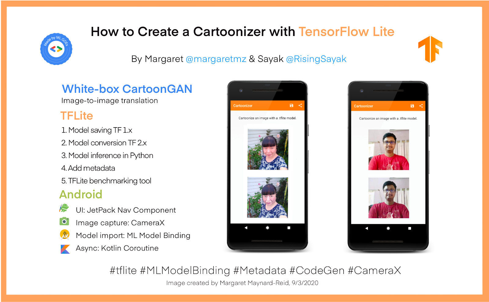
A guest post by ML GDEs Margaret Maynard-Reid (Tiny Peppers) and Sayak Paul (PyImageSearch)

This is an end-to-end tutorial on how to convert a TensorFlow model to TensorFlow Lite (TFLite) and deploy it to an Android app for cartoonizing an image captured by the camera.

We created this end-to-end tutorial to help developers with these objectives:

  • Provide a reference for the developers looking to convert models written in TensorFlow 1.x to their TFLite variants using the new features of the latest (v2) converter — for example, the MLIR-based converter, more supported ops, and improved kernels, etc.
    (In order to convert TensorFlow 2.x models in TFLite please follow this guide.)
  • How to download the .tflite models directly from TensorFlow Hub if you are only interested in using the models for deployment.
  • Understand how to use the TFLite tools such as the Android Benchmark Tool, Model Metadata, and Codegen.
  • Guide developers on how to create a mobile application with TFLite models easily, with ML Model Binding feature from Android Studio.

Please follow along with the notebooks here for model saving/conversion, populating metadata; and the Android code on GitHub here. If you are not familiar with the SavedModel format, please refer to the TensorFlow documentation for details. While this tutorial discusses the steps of how to create the TFLite models , feel free to download them directly from TensorFlow Hub here and get started using them in your own applications.
White-box CartoonGAN is a type of generative adversarial network that is capable of transforming an input image (preferably a natural image) to its cartoonized representation. The goal here is to produce a cartoonized image from an input image that is visually and semantically aesthetic. For more details about the model check out the paper Learning to Cartoonize Using White-box Cartoon Representations by Xinrui Wang and Jinze Yu. For this tutorial, we used the generator part of White-box CartoonGAN.

Create the TensorFlow Lite Model

The authors of White-box CartoonGAN provide pre-trained weights that can be used for making inference on images. However, those weights are not ideal if we were to develop a mobile application without having to make API calls to fetch them. This is why we will first convert these pre-trained weights to TFLite which would be much more suitable to go inside a mobile application. All of the code discussed in this section is available on GitHub here. Here is a step-by-step summary of what we will be covering in this section:

  • Generate a SavedModel out of the pre-trained model checkpoints.
  • Convert SavedModel with post-training quantization using the latest TFLiteConverter.
  • Run inference in Python with the converted model.
  • Add metadata to enable easy integration with a mobile app.
  • Run model benchmark to make sure the model runs well on mobile.

Generate a SavedModel from the pre-trained model weights

The pre-trained weights of White-box CartoonGAN come in the following format (also referred to as checkpoints) –

├── checkpoint
├── model-33999.data-00000-of-00001
└── model-33999.index

As the original White-box CartoonGAN model is implemented in TensorFlow 1, we first need to generate a single self-contained model file in the SavedModel format using TensorFlow 1.15. Then we will switch to TensorFlow 2 later to convert it to the lightweight TFLite format. To do this we can follow this workflow –

  • Create a placeholder for the model input.
  • Instantiate the model instance and run the input placeholder through the model to get a placeholder for the model output.
  • Load the pre-trained checkpoints into the current session of the model.
  • Finally, export to SavedModel.

Note that the aforementioned workflow will be based on TensorFlow 1.x.
This is how all of this looks in code in TensorFlow 1.x:

with tf.Session() as sess:
input_photo = tf.placeholder(tf.float32, [1, None, None, 3], name='input_photo')

network_out = network.unet_generator(input_photo)
final_out = guided_filter.guided_filter(input_photo, network_out, r=1, eps=5e-3)
final_out = tf.identity(final_out, name='final_output')

all_vars = tf.trainable_variables()
gene_vars = [var for var in all_vars if 'generator' in var.name]
saver = tf.train.Saver(var_list=gene_vars)
sess.run(tf.global_variables_initializer())
saver.restore(sess, tf.train.latest_checkpoint(model_path))

# Export to SavedModel
tf.saved_model.simple_save(
sess,
saved_model_directory,
inputs={input_photo.name: input_photo},
outputs={final_out.name: final_out}
)

Now that we have the original model in the SavedModel format, we can switch to TensorFlow 2 and proceed toward converting it to TFLite.

Convert SavedModel to TFLite

TFLite provides support for three different post-training quantization strategies

  • Dynamic range
  • Float16
  • Integer

Based on one’s use-case a particular strategy is determined. In this tutorial, however, we will be covering all of these different quantization strategies to give you a fair idea.

TFLite models with dynamic-range and float16 quantization

The steps to convert models to TFLite using these two quantization strategies are almost identical except during float16 quantization, you need to specify an extra option. The steps for model conversion are demonstrated in the code below –

# Create a concrete function from the SavedModel 
model = tf.saved_model.load(saved_model_dir)
concrete_func = model.signatures[
tf.saved_model.DEFAULT_SERVING_SIGNATURE_DEF_KEY]

# Specify the input shape
concrete_func.inputs[0].set_shape([1, IMG_SHAPE, IMG_SHAPE, 3])

# Convert the model and export
converter = tf.lite.TFLiteConverter.from_concrete_functions([concrete_func])
converter.optimizations = [tf.lite.Optimize.DEFAULT]
converter.target_spec.supported_types = [tf.float16] # Only for float16
tflite_model = converter.convert()
open(tflite_model_path, 'wb').write(tflite_model)

A couple of things to note from the code above –

  • Here, we are specifying the input shape of the model that will be converted to TFLite. However, note that TFLite supports dynamic shaped models from TensorFlow 2.3. We used fixed-shaped inputs in order to restrict the memory usage of the models running on mobile devices.
  • In order to convert the model using dynamic-range quantization, one just needs to comment this line converter.target_spec.supported_types = [tf.float16].

TFLite models with integer quantization

In order to convert the model using integer quantization, we need to pass a representative dataset to the converter so that the activation ranges can be calibrated accordingly. TFLite models generated using this strategy are known to sometimes work better than the other two that we just saw. Integer quantized models are generally smaller as well.
For the sake of brevity, we are going to skip the representative dataset generation part but you can refer to it in this notebook.
In order to let the TFLiteConverter take advantage of this strategy, we need to just pass converter.representative_dataset = representative_dataset_gen and remove converter.target_spec.supported_types = [tf.float16].
So after we generated these different models here’s how we stand in terms of model size – You might feel tempted to just go with the model quantized with integer quantization but you should also consider the following things before finalizing this decision –

  • Quality of the end results of the models.
  • Inference time (the lower the better).
  • Hardware accelerator compatibility.
  • Memory usage.

We will get to these in a moment. If you want to dig deeper into these different quantization strategies refer to the official guide here.
These models are available on TensorFlow Hub and you can find them here.

Running inference in Python

After you have generated the TFLite models, it is important to make sure that models perform as expected. A good way to ensure that is to run inference with the models in Python before integrating them in mobile applications.
Before feeding an image to our White-box CartoonGAN TFLite models it’s important to make sure that the image is preprocessed well. Otherwise, the models might perform unexpectedly. The original model was trained using BGR images, so we need to account for this fact in the preprocessing steps as well. You can find all of the preprocessing steps in this notebook.
Here is the code to use a TFLite model for making inference on a preprocessed input image –

interpreter = tf.lite.Interpreter(model_path=tflite_model_path)
input_details = interpreter.get_input_details()

interpreter.allocate_tensors()
interpreter.set_tensor(input_details[0]['index'],
preprocessed_source_image)
interpreter.invoke()

raw_prediction = interpreter.tensor(
interpreter.get_output_details()[0]['index'])()

As mentioned above, the output would be an image but with BGR channel ordering which might not be visually appropriate. So, we would need to account for that fact in the postprocessing steps.
After the postprocessing steps are incorporated here is how the final image would look like alongside the original input image – Again, you can find all of the postprocessing steps in this notebook.

Add metadata for easy integration with a mobile app

Model metadata in TFLite makes the life of mobile application developers much easier. If your TFLite model is populated with the right metadata then it becomes a matter of only a few keystrokes to integrate that model into a mobile application. Discussing the code to populate a TFLite model with metadata is out of the scope for this tutorial, and please refer to the metadata guide. But in this section, we are going to provide you with some of the important pointers about metadata population for the TFLite models we generated. You can follow this notebook to refer to all the code. Two of the most important parameters we discovered during metadata population are mean and standard deviation with which the results should be processed. In our case, mean and standard deviation need to be used for both preprocessing postprocessing. For normalizing the input image the metadata configuration should be like the following –

input_image_normalization.options.mean = [127.5]
input_image_normalization.options.std = [127.5]

This would make the pixel range in an input image to [-1, 1]. Now, during postprocessing, the pixels need to be scaled back to the range of [0, 255]. For this, the configuration would go as follows –

output_image_normalization.options.mean = [-1]
output_image_normalization.options.std = [0.00784313] # 1/127.5

There are two files created from the “add metadata process”:

  • A .tflite file with the same name as the original model, with metadata added, including model name, description, version, input and output tensor, etc.
  • To help to display metadata, we also export the metadata into a .json file so that you can print it out. When you import the model into Android Studio, metadata can be displayed as well.

The models that have been populated with metadata make it really easy to import in Android Studio which we will discuss later under the “Model deployment to an Android” section.

Benchmark models on Android (Optional)

As an optional step, we used the TFLite Android Model Benchmark tool to get an idea of the runtime performance on Android before deploying it.
There are two options of using the benchmark tool, one with a C++ binary running in background and another with an Android APK running in foreground.
Here ia a high-level summary using the benchmark C++ binary:
1. Configure Android SDK/NDK prerequisites
2. Build the benchmark C++ binary with bazel

bazel build -c opt 
--config=android_arm64
tensorflow/lite/tools/benchmark:benchmark_model

3. Use adb (Android Debug Bridge) to push the benchmarking tool binary to device and make executable

adb push benchmark_model /data/local tmp
adb shell chmod +x /data/local/tmp/benchmark_model

4. Push the whitebox_cartoon_gan_dr.tflite model to device

adb push whitebox_cartoon_gan_dr.tflite /data/local/tmp

5. Run the benchmark tool

adb shell /data/local/tmp/android_aarch64_benchmark_model        
--graph=/data/local/tmp/whitebox_cartoon_gan_dr.tflite
--num_threads=4

You will see a result in the terminal like this: Repeat above steps for the other two tflite models: float16 and int8 variants.
In summary, here is the average inference time we got from the benchmark tool running on a Pixel 4: Refer to the documentation of the benchmark tool (C++ binary | Android APK) for details and additional options such as how to reduce variance between runs and how to profile operators, etc. You can also see the performance values of some of the popular ML models on the TensorFlow official documentation here.

Model deployment to Android

Now that we have the quantized TensorFlow Lite models with metadata by either following the previous steps (or by downloading the models directly from TensorFlow Hub here), we are ready to deploy them to Android. Follow along with the Android code on GitHub here.
The Android app uses Jetpack Navigation Component for UI navigation and CameraX for image capture. We use the new ML Model Binding feature for importing the tflite model and then Kotlin Coroutine for async handling of the model inference so that the UI is not blocked while waiting for the results.
Let’s dive into the details step by step:

  • Download Android Studio 4.1 Preview.
  • Create a new Android project and set up the UI navigation.
  • Set up the CameraX API for image capture.
  • Import the .tflite models with ML Model Binding.
  • Putting everything together.

Download Android Studio 4.1 Preview

We need to first install Android Studio Preview (4.1 Beta 1) in order to use the new ML Model Binding feature to import a .tflite model and auto code generation. You can then explore the tfllite models visually and most importantly use the generated classes directly in your Android projects.
Download the Android Studio Preview here. You should be able to run the Preview version side by side with a stable version of Android Studio. Make sure to update your Gradle plug-in to at least 4.1.0-alpha10; otherwise the ML Model Binding menu may be inaccessible.

Create a new Android Project

First let’s create a new Android project with an empty Activity called MainActivity.kt which contains a companion object that defines the output directory where the captured image will be stored.
Use Jetpack Navigation Component to navigate the UI of the app. Please refer to the tutorial here to learn more details about this support library.
There are 3 screens in this sample app:

  • PermissionsFragment.kt handles checking the camera permission.
  • CameraFragment.kt handles camera setup, image capture and saving.
  • CartoonFragment.kt handles the display of input and cartoon image in the UI.

The navigation graph in nav_graph.xml defines the navigation of the three screens and data passing between CameraFragment and CartoonFragment.

Set up CameraX for image capture

CameraX is a Jetpack support library which makes camera app development much easier.
Camera1 API was simple to use but it lacked a lot of functionality. Camera2 API provides more fine control than Camera1 but it’s very complex — with almost 1000 lines of code in a very basic example.
CameraX on the other hand, is much easier to set up with 10 times less code. In addition, it’s lifecycle aware so you don’t need to write the extra code to handle the Android lifecycle.
Here are the steps to set up CameraX for this sample app:

  • Update build.gradle dependencies
  • Use CameraFragment.kt to hold the CameraX code
  • Request camera permission
  • Update AndroidManifest.ml
  • Check permission in MainActivity.kt
  • Implement a viewfinder with the CameraX Preview class
  • Implement image capture
  • Capture an image and convert it to a Bitmap

CameraSelector is configured to be able to take use of the front facing and rear facing camera since the model can stylize any type of faces or objects, and not just a selfie.
Once we capture an image, we convert it to a Bitmap which is passed to the TFLite model for inference. Navigate to a new screen CartoonFragment.kt where both the original image and the cartoonized image are displayed.

Import the TensorFlow Lite models

Now that the UI code has been completed. It’s time to import the TensorFlow Lite model for inference. ML Model Binding takes care of this with ease. In Android Studio, go to File > New > Other > TensorFlow Lite Model:

  • Specify the .tflite file location.
  • “Auto add build feature and required dependencies to gradle” is checked by default.
  • Make sure to also check “Auto add TensorFlow Lite gpu dependencies to gradle” since the GAN models are complex and slow, and so we need to enable GPU delegate.

This import accomplishes two things:

  • automatically create a ml folder and place the model file .tflite file under there.
  • auto generate a Java class under the folder: app/build/generated/ml_source_out/debug/[package-name]/ml, which handles all the tasks such as model loading, image pre-preprocess and post-processing, and run model inference for stylizing the input image.

Once the import completes, we see the *.tflite display the model metadata info as well as code snippets in both Kotlin and Java that can be copy/pasted in order to use the model: Repeat the steps above to import the other two .tflite model variants.

Putting everything together

Now that we have set up the UI navigation, configured CameraX for image capture, and the tflite models are imported, let’s put all the pieces together!

  • Model input: capture a photo with CameraX and save it
  • Run inference on the input image and create a cartoonized version
  • Display both the original photo and the cartoonized photo in the UI
  • Use Kotlin coroutine to prevent the model inference from blocking UI main thread

First we capture a photo with CameraX in CameraFragment.kt under imageCaptue?.takePicture(), then in ImageCapture.OnImageSavedCallback{}, onImageSaved() convert the .jpg image to a Bitmap, rotate if necessary, and then save it to an output directory defined in MainActivity earlier.
With the JetPack Nav Component, we can easily navigate to CartoonFragment.kt and pass the image directory location as a string argument, and the type of tflite model as an integer. Then in CartoonFragment.kt, retrieve the file directory string where the photo was stored, create an image file then convert it to be Bitmap which can be used as the input to the tflite model.
In CartoonFragment.kt, also retrieve the type of tflite model that was chosen for inference. Run model inference on the input image and create a cartoon image. We display both the original image and the cartoonized image in the UI.
Note: the inference takes time so we use Kotlin coroutine to prevent the model inference from blocking the UI main thread. Show a ProgressBar till the model inference completes.
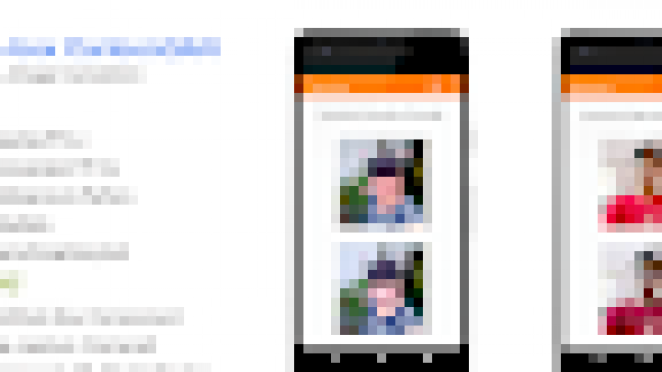
Here is what we have once all pieces are put together and here are the cartoon images created by the model: This brings us to the end of the tutorial. We hope you have enjoyed reading it and will apply what you learned to your real-world applications with TensorFlow Lite. If you have created any cool samples with what you learned here, please remember to add it to awesome-tflite – a repo with TensorFlow Lite samples, tutorials, tools and learning resources.

Acknowledgments

This Cartoonizer with TensorFlow Lite project with end-to-end tutorial was created with the great collaboration by ML GDEs and the TensorFlow Lite team. This is the one of a series of end-to-end TensorFlow Lite tutorials. We would like to thank Khanh LeViet and Lu Wang (TensorFlow Lite), Hoi Lam (Android ML), Trevor McGuire (CameraX) and Soonson Kwon (ML GDEs Google Developers Experts Program), for their collaboration and continuous support.
Also thanks to the authors of the paper Learning to Cartoonize Using White-box Cartoon Representations: Xinrui Wang and Jinze Yu.
When developing applications, it’s important to consider recommended practices for responsible innovation; check out Responsible AI with TensorFlow for resources and tools you can use. Read More