Reducing training time with Apache MXNet and Horovod on Amazon SageMaker

Reducing training time with Apache MXNet and Horovod on Amazon SageMaker

Amazon SageMaker is a fully managed service that provides every developer and data scientist with the ability to build, train, and deploy machine learning (ML) models quickly. Amazon SageMaker removes the heavy lifting from each step of the ML process to make it easier to develop high-quality models. As datasets continue to increase in size, additional compute is required to reduce the amount of time it takes to train. One method to scale horizontally and add these additional resources on Amazon SageMaker is through the use of Horovod and Apache MXNet. In this post, we show how you can reduce training time with MXNet and Horovod on Amazon SageMaker. We also demonstrate how to further improve performance with advanced sections on Horovod autotuning, Horovod Timeline, Horovod Fusion, and MXNet optimization.

Distributed training

Distributed training of neural networks for computer vision (CV) and natural language processing (NLP) applications has become ubiquitous. With Apache MXNet, you only need to modify a few lines of code to enable distributed training.

Distributed training allows you to reduce training time by scaling horizontally. The goal is to split training tasks into independent subtasks and run these across multiple devices. There are primarily two approaches for training in parallel:

  • Data parallelism – You distribute the data and share the model across multiple compute resources
  • Model parallelism – You distribute the model and share transformed data across multiple compute resources.

In this post, we focus on data parallelism. Specifically, we discuss how Horovod and MXNet allow you to train efficiently on Amazon SageMaker.

Horovod overview

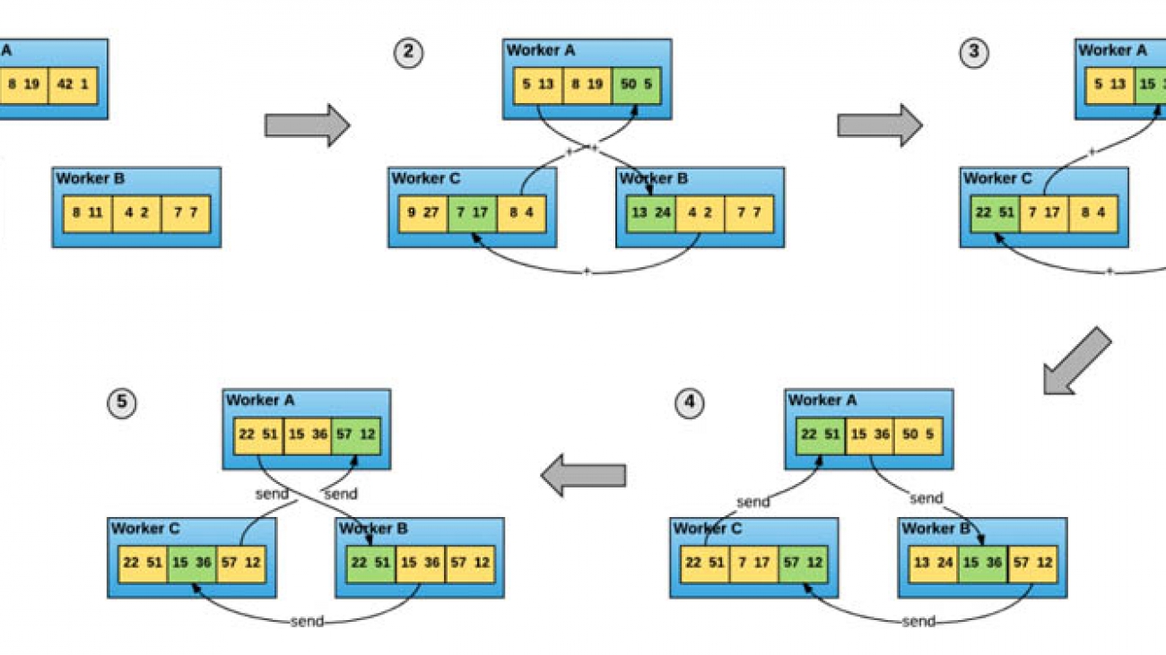
Horovod is an open-source distributed deep learning framework. It uses efficient inter-GPU and inter-node communication methods such as NVIDIA Collective Communications Library (NCCL) and Message Passing Interface (MPI) to distribute and aggregate model parameters between workers. Horovod makes distributed deep learning fast and easy by using a single-GPU training script and scaling it across many GPUs in parallel. It’s built on top of the ring-allreduce communication protocol. This approach allows each training process (such as a process running on a single GPU device) to talk to its peers and exchange gradients by averaging (called reduction) on a subset of gradients. The following diagram illustrates how ring-allreduce works.


Fig. 1 The ring-allreduce algorithm allows worker nodes to average gradients and disperse them to all nodes without the need for a parameter server (
source)

Apache MXNet is integrated with Horovod through the distributed training APIs defined in Horovod, and you can convert the non-distributed training by following the higher level code skeleton, which we show in this post.

Although this greatly simplifies the process of using Horovod, you must consider other complexities. For example, you may need to install additional software and libraries to resolve your incompatibilities for making distributed training work. Horovod requires a certain version of Open MPI, and if you want to use high-performance training on NVIDIA GPUs, you need to install NCCL libraries. These complexities are amplified when you scale across multiple devices, because you need to make sure all the software and libraries in the new nodes are properly installed and configured. Amazon SageMaker includes all the required libraries to run distributed training with MXNet and Horovod. Prebuilt Amazon SageMaker Docker images come with popular open-source deep learning frameworks and pre-configured CUDA, cuDNN, MPI, and NCCL libraries. Amazon SageMaker manages the difficult process of properly installing and configuring your cluster. Amazon SageMaker and MXNet simplify training with Horovod by managing the complexities to support distributed training at scale.

Test problem and dataset

To benchmark the efficiencies realized by Horovod, we trained the notoriously resource-intensive model architectures Mask-RCNN and Faster-RCNN. These model architectures were first introduced in 2018 and 2016, respectively, and are currently considered the baseline model architectures for two popular CV tasks: instance segmentation (Mask-RCNN) and object detection (Faster-RCNN). Mask-RCNN builds upon Faster-RCNN by adding a mask for segmentation. Apache MXNet provides pre-built Mask-RCNN and Faster-RCNN models as part of the GluonCV model zoo, simplifying the process of training these models.

To train our object detection and instance segmentation models, we used the popular COCO2017 dataset. This dataset provides more than 200,000 images and their corresponding labels. The COCO2017 dataset is considered an industry standard for benchmarking CV models.

GluonCV is a CV toolkit built on top of MXNet. It provides out-of-the-box support for various CV tasks, including data loading and preprocessing for many common algorithms available within its model zoo. It also provides a tutorial on getting the COCO2017 dataset.

To make this process replicable for Amazon SageMaker users, we show an entire end-to-end process for training Mask-RCNN and Faster-RCNN with Horovod and MXNet. To begin, we first open the Jupyter environment in your Amazon SageMaker notebook and use the conda_mxnet_p36 kernel. Next, we install the required Python packages:

! pip install gluoncv
! pip install pycocotools

We use the GluonCV toolkit to download the COCO2017 dataset onto our Amazon SageMaker notebook:

import gluoncv as gcv
gcv.utils.download('https://gluon-cv.mxnet.io/_downloads/b6ade342998e03f5eaa0f129ad5eee80/mscoco.py',path='./')
#Now to install the dataset. Warning, this may take a while
! python mscoco.py --download-dir data

We upload COCO2017 to the specified Amazon Simple Storage Service (Amazon S3) bucket using the following command:

! aws s3 cp './data/' s3://<INSERT BUCKET NAME>/ --recursive –quiet

Training script with Horovod Support

To use Horovod in your training script, you only need to make a few modifications. For code samples and instructions, see Horovod with MXNet. In addition, many GluonCV models in the model zoo have scripts that already support Horovod out of the box. In this section, we review the key changes required for Horovod to correctly work on Amazon SageMaker with Apache MXNet. The following code follows directly from the Horovod documentation:

import mxnet as mx
import horovod.mxnet as hvd
from mxnet import autograd

# Initialize Horovod, this has to be done first as it activates Horovod.
hvd.init()

# GPU setup 
context =[mx.gpu(hvd.local_rank())] #local_rank is the specific gpu on that 
# instance
num_gpus = hvd.size() #This is how many total GPUs you will be using.

#Typically, in your data loader you will want to shard your dataset. For 
# example, in the train_mask_rcnn.py script 
train_sampler = 
        gcv.nn.sampler.SplitSortedBucketSampler(...,
                                                num_parts=hvd.size() if args.horovod else 1,
                                                part_index=hvd.rank() if args.horovod else 0)

#Normally, we would shard the dataset first for Horovod.
val_loader = mx.gluon.data.DataLoader(dataset, len(ctx), ...) #... is for your # other arguments

    
# You build and initialize your model as usual.
model = ...

# Fetch and broadcast the parameters.
params = model.collect_params()
if params is not None:
    hvd.broadcast_parameters(params, root_rank=0)

# Create DistributedTrainer, a subclass of gluon.Trainer.
trainer = hvd.DistributedTrainer(params, opt)

# Create loss function and train your model as usual. 

Training job configuration

The Amazon SageMaker MXNet estimator class supports Horovod via the distributions parameter. We need to add a predefined mpi parameter with the enabled flag, and define the following additional parameters:

  • processes_per_host (int) – Number of processes MPI should launch on each host. This parameter is usually equal to the number of GPU devices available on any given instance.
  • custom_mpi_options (str) – Any custom mpirun flags passed in this field are added to the mpirun command and run by Amazon SageMaker for Horovod training.

The follow example code initializes the distributions parameters:

distributions = {'mpi': {
                    'enabled': True,
                    'processes_per_host': 8, #Each instance has 8 gpus
			'custom_mpi_options': '-verbose --NCCL_DEBUG=INFO'
                        }
                }

Next, we need to configure other parameters of our training job, such as hyperparameters, and the input and output Amazon S3 locations. To do this, we use the MXNet estimator class from the Amazon SageMaker Python SDK:

#Define the basic configuration of your Horovod-enabled Sagemaker training 
# cluster.
num_instances = 2 # How many nodes you want to use.
instance_family = 'ml.p3dn.24xlarge' # Which instance type you want to use.


estimator = MXNet(
                entry_point=<source_name>.py,         #Script entry point.
                source_dir='./source',                #Script Location
                role=role, 
                train_instance_type=instance_family,
                train_instance_count=num_instances,
                framework_version='1.6.0',            #MXNet version.
                train_volume_size=100,                #Size for the dataset.
                py_version='py3',                     #Python version.
                hyperparameters=hyperparameters,
                distributions=distributions           #For use with Horovod.

We’re now ready to start our first Horovod-powered training job with the following command:

            estimator.fit(
                {'data':'s3://' + bucket_name + '/data'}
            )

Results

We performed these benchmarks on two similar GPU instance types: the p3.16xlarge and the more powerful p3dn.24xlarge. Although both have 8 NVIDIA V100 GPUs, the latter instance is designed with distributed training in mind. In addition to a high-throughput network interface amenable to the inter-node data transfers inherent in distributed training, the p3dn.24xlarge boasts more compute and additional memory over the p3.16xlarge.

We ran benchmarks in three different use cases. In the first and second use cases, we trained the models on a single instance using all 8 local GPUs, to demonstrate the efficiencies gained by using Horovod to manage local training across multiple GPUs. In the third use case, we used Horovod for distributed training across multiple instances, each with 8 local GPUs, to demonstrate the additional efficiency increase by scaling horizontally.

The following table summarizes the time and accuracy for each training scenario.

Model Instance Type 1 Instance, 8 GPUs w/o Horovod 1 Instance, 8 GPUs with Horovod 3 Instances, 8 GPUs with Horovod
Training Time Accuracy Training Time Accuracy Training Time Accuracy
Faster RCNN p3.16xlarge 35 h 47 m 37.6 8 h 26 m 37.5 4 h 58 m 37.4
Faster RCNN p3dn.24xlarge 32 h 24 m 37.5 7 h 27 m 37.5 3 h 37 m 37.3
Mask RCNN p3.16xlarge 45 h 28 m

38.5 (bbox)

34.8 (segm)

10 h 28 m

34.4 (bbox)

31.3 (segm)

5 h 34 m

36.8 (bbox)

33.5 (segm)

Mask RCNN p3dn.24xlarge 40 h 49 m

38.3 (bbox)

34.8 (segm)

8 h 41 m 34.6 (bbox)
31.5 (segm)
4 h 2 m

37.0 (bbox)

33.4 (segm)

Table 1: Training time and accuracy are shown for three different training scenarios.

As expected, when using Horovod to distribute training across multiple instances, the time to convergence is significantly reduced. Additionally, even when training on a single instance, Horovod substantially increases training efficiency when using multiple local GPUs, as compared to the default parameter-server approach. Horovod’s simplified APIs and abstractions enable you to unlock efficiency gains when training across multiple GPUs, both on a single machine or many. For more information about using this approach for scaling batch size and learning rate, see Accurate, Large Minibatch SGD: Training ImageNet in 1 Hour.

With the improvement in training time enabled by Horovod and Amazon SageMaker, you can focus more on improving your algorithms instead of waiting for jobs to finish training. You can train in parallel across multiple instances with marginal impact to mean Average Precision (mAP).

Optimizing Horovod training

Horovod provides several additional utilities that allow you to analyze and optimize training performance.

Horovod autotuning

Finding the optimal combinations of parameters for a given combination of model and cluster size may require several iterations of trial and error.

The autotune feature allows you to automate this trial-and-error activity within a single training job, and uses Bayesian optimization to search through the parameter space for the most performant combination of parameters. Horovod searches for the best combination of parameters in the first cycles of a training job. When it defines the best combination, Horovod writes it in the autotune log and uses this combination for the remainder of the training job. For more information, see Autotune: Automated Performance Tuning.

To enable autotuning and capture the search log, pass the following parameters in your MPI configuration:

{
    'mpi':
    {
        'enabled': True,
        'custom_mpi_options': '-x HOROVOD_AUTOTUNE=1 -x         HOROVOD_AUTOTUNE_LOG=/opt/ml/output/autotune_log.csv'
    }
}

Horovod Timeline

Horovod Timeline is a report available after training completion that captures all activities in the Horovod ring. This is useful to understand which operations are taking the longest and identify optimization opportunities. For more information, see Analyze Performance.

To generate a timeline file, add the following parameters in your MPI command:

{
    'mpi':
    {
        'enabled': True,
        'custom_mpi_options': '-x HOROVOD_TIMELINE=/opt/ml/output/timeline.json'
    }
}

The /opt/ml/output is a directory with a specific purpose. After the training job is complete, Amazon SageMaker automatically archives all files in this directory and uploads it to an Amazon S3 location that you define in the Python Amazon SageMaker SDK API.

Tensor Fusion

The Tensor Fusion feature allows you to perform batch allreduce operations at training time. This typically results in better overall performance. For more information, see Tensor Fusion. By default, Tensor Fusion is enabled and has a buffer size of 64 MB. You can modify buffer size using a custom MPI flag as follows (for our use case, we override the default 64 MB buffer value with 32 MB):

{
    'mpi':
    {
        'enabled': True,
        'custom_mpi_options': '-x HOROVOD_FUSION_THRESHOLD=33554432'
    }
}

You can also adjust batch cycles using the HOROVOD_CYCLE_TIME parameter. Cycle time is defined in milliseconds. See the following code:

{
    'mpi':
    {
        'enabled': True,
        'custom_mpi_options': '-x HOROVOD_CYCLE_TIME=5'
    }
}

Optimizing MXNet models

Another optimization technique is related to optimizing the MXNet model itself. We recommend running the code with os.environ['MXNET_CUDNN_AUTOTUNE_DEFAULT'] = '1'. Then you can copy the best OS environment variables for future training. In our testing, we found the following to be the best results:

os.environ['MXNET_GPU_MEM_POOL_TYPE'] = 'Round'
os.environ['MXNET_GPU_MEM_POOL_ROUND_LINEAR_CUTOFF'] = '26'
os.environ['MXNET_EXEC_BULK_EXEC_MAX_NODE_TRAIN_FWD'] = '999'
os.environ['MXNET_EXEC_BULK_EXEC_MAX_NODE_TRAIN_BWD'] = '25'
os.environ['MXNET_GPU_COPY_NTHREADS'] = '1'
os.environ['MXNET_OPTIMIZER_AGGREGATION_SIZE'] = '54'

Conclusion

In this post, we demonstrated how to reduce training time with Horovod and Apache MXNet on Amazon SageMaker. You can train your model out of the box without worrying about any additional complexities.

For more information about deep learning and MXNet, see the MXNet crash course and Dive into Deep Learning book. You can also get started on the MXNet website and MXNet GitHub examples directory. If you’re new to distributed training and want to dive deeper, we highly recommend reading the paper Horovod: fast and easy distributed deep learning in TensorFlow. If you use the AWS Deep Learning Containers and AWS Deep Learning AMIs, you can learn how to set up this workflow in that environment in our recent post How to run distributed training using Horovod and MXNet on AWS DL containers and AWS Deep Learning AMIs.


About the Authors

Vadim Dabravolski is AI/ML Solutions Architect with FinServe team. He is focused on Computer Vision and NLP technologies and how to apply them to business use cases. After hours Vadim enjoys jogging in NYC boroughs, reading non-fiction (business, history, culture, politics, you name it), and rarely just doing nothing.


Corey Barrett is a Data Scientist in the Amazon ML Solutions Lab. As a member of the ML Solutions Lab, he leverages Machine Learning and Deep Learning to solve critical business problems for AWS customers. Outside of work, you can find him enjoying the outdoors, sipping on scotch, and spending time with his family.


Chaitanya Bapat is a Software Engineer with the AWS Deep Learning team. He works on Apache MXNet and integrating the framework with Amazon Sagemaker, DLC and DLAMI. In his spare time, he loves watching sports and enjoys reading books and learning Spanish.


Karan Jariwala is a Software Development Engineer on the AWS Deep Learning team. His work focuses on training deep neural networks. Outside of work, he enjoys hiking, swimming, and playing tennis.


Read More

More Space, Less Jam: Transportation Agency Uses NVIDIA DRIVE for Federal Highway Pilot

More Space, Less Jam: Transportation Agency Uses NVIDIA DRIVE for Federal Highway Pilot

It could be just a fender bender or an unforeseen rain shower, but a few seconds of disruption can translate to extra minutes or even hours of mind-numbing highway traffic.

But how much of this congestion could be avoided with AI at the wheel?

That’s what the Contra Costa Transportation Authority is working to determine in one of three federally funded automated driving system pilots in the next few years. Using vehicles retrofitted with the NVIDIA DRIVE AGX Pegasus platform, the agency will estimate just how much intelligent transportation can improve the efficiency of everyday commutes.

“As the population grows, there are more demands on roadways and continuing to widen them is just not sustainable,” said Randy Iwasaki, executive director of the CCTA. “We need to find better ways to move people, and autonomous vehicle technology is one way to do that.”

The CCTA was one of eight awardees – and the only local agency – of the Automated Driving System Demonstration Grants Program from the U.S. Department of Transportation, which aims to test the safe integration of self-driving cars into U.S. roads.

The Bay Area agency is using the funds for the highway pilot, as well as two other projects to develop robotaxis equipped with self-docking wheelchair technology and test autonomous shuttles for a local retirement community.

A More Intelligent Interstate

From the 101 to the 405, California is known for its constantly congested highways. In Contra Costa, Interstate 680 is one of those high-traffic corridors, funneling many of the area’s 120,000 daily commuters. This pilot will explore how the Highway Capacity Manual – which sets assumptions for modeling freeway capacity – can be updated to incorporate future automated vehicle technology.

Iwasaki estimates that half of California’s congestion is recurrent, meaning demand for roadways is higher than supply.  The other half is non-recurrent and can be attributed to things like weather events, special events — such as concerts or parades — and accidents. By eliminating human driver error, which has been estimated by the National Highway Traffic Safety Administration to be the cause of 94 percent of traffic accidents, the system becomes more efficient and reliable.

Autonomous vehicles don’t get distracted or drowsy, which are two of the biggest causes of human error while driving. They also use redundant and diverse sensors as well as high-definition maps to detect and plan the road ahead much farther than a human driver can.

These attributes make it easier to maintain constant speeds as well as space for vehicles to merge in and out of traffic for a smoother daily commute.

Driving Confidence

The CCTA will be using a fleet of autonomous test vehicles retrofitted with sensors and NVIDIA DRIVE AGX to gauge how much this technology can improve highway capacity.

The NVIDIA DRIVE AGX Pegasus AI compute platform uses the power of two Xavier systems-on-a-chip and two NVIDIA Turing architecture GPUs to achieve an unprecedented 320 trillion operations per second of supercomputing performance. The platform is designed and built for Level 4 and Level 5 autonomous systems, including robotaxis.

NVIDIA DRIVE AGX Pegasus

Iwasaki said the agency tapped NVIDIA for this pilot because the company’s vision matches its own: to solve real problems that haven’t been solved before, using proactive safety measures every step of the way.

With half of adult drivers reporting they’re fearful of self-driving technology, this approach to autonomous vehicles is critical to gaining public acceptance, he said.

“We need to get the word out that this technology is safer and let them know who’s behind making sure it’s safer,” Iwasaki said.

The post More Space, Less Jam: Transportation Agency Uses NVIDIA DRIVE for Federal Highway Pilot appeared first on The Official NVIDIA Blog.

Read More

AI From the Sky: Stealth Entrepreneur’s Drone Platform Sees into Mines

AI From the Sky: Stealth Entrepreneur’s Drone Platform Sees into Mines

Christian Sanz isn’t above trying disguises to sneak into places. He once put on a hard hat, vest and steel-toed boots to get onto the construction site of the San Francisco 49ers football stadium to explore applications for his drone startup.

That bold move scored his first deal.

For the entrepreneur who popularized drones in hackathons in 2012 as founder of the Drone Games matches, starting Skycatch in 2013 was a logical next step.

“We decided to look for more industrial uses, so I went and bought construction gear and was able to blend in, and in many cases people didn’t know I wasn’t working for them as I was collecting data,” Sanz said.

Skycatch has since grown up: In recent years the San Francisco-based company has been providing some of the world’s largest mining and construction companies its AI-enabled automated drone surveying and analytics platform. The startup, which has landed $47 million in funding, promises customers automated visibility over operations.

At the heart of the platform is the NVIDIA Jetson TX2-driven Edge1 edge computer and base station. It can create 2D maps and 3D point clouds in real-time, as well as pinpoint features  to within five-centimeter accuracy. Also, it runs AI models to do split-second inference in the field to detect objects.

Today, Skycatch announced its new Discover1 device. The Discover1 connects to industrial machines, enabling customers to plug in a multitude of sensors that can expand the data gathering of Skycatch.

The Discover1 sports a Jetson Nano inside to facilitate the collection of data from sensors and enable computer vision and machine learning on the edge. The device has LTE and WiFi connectivity to stream data to the cloud.

Changing-Tracking AI

Skycatch can capture 3D images of job sites for merging against blueprints to monitor changes.

Such monitoring for one large construction site showed that electrical conduit pipes were installed in the wrong spot. Concrete would be poured next, cementing them in place. Catching the mistake early helped avoid a much costlier revision later.

Skycatch says that customers using its services can expect to compress the timelines on their projects as well as reduce costs by catching errors before they become bigger problems.

Surveying with Speed

Japan’s Komatsu, one of the world’s leading makers of bulldozers, excavators and other industrial machines, is an early customer of Skycatch.

With Japan facing a labor shortage, the equipment maker was looking for ways to help automate its products. One bottleneck was surveying a location, which could take days, before unleashing the machines.

Skycatch automated the process with its drone platform. The result for Komatsu is that less-skilled workers can generate a 3D map of a job site within 30 minutes, enabling operators to get started sooner with the land-moving beasts.

Jetson for AI

As Skycatch was generating massive sums of data, the company’s founder realized they needed more computing capability to handle it. Also, given the environment in which they were operating, the computing had to be done on the edge while consuming minimal power.

They turned to the Jetson TX2, which provides server-level AI performance using the CUDA-enabled NVIDIA Pascal GPU in a small form factor and taps as little as 7.5 watts of power. It’s high memory bandwidth and wide range of hardware interfaces in a rugged form factor are ideal for the industrial environments Skycatch operates in.

Sanz says that “indexing the physical world” is demanding because of all the unstructured data of photos and videos, which require feature extraction to “make sense of it all.”

“When the Jetson TX2 came out, we were super excited. Since 2017, we’ve rewritten our photogrammetry engine to use the CUDA language framework so that we can achieve much faster speed and processing,” Sanz said.

Remote Bulldozers

The Discover1 can collect data right from the shovel of a bulldozer. Inertial measurement unit, or IMU, sensors can be attached to the Discover1 on construction machines to track movements from the bulldozer’s point of view.

One of the largest mining companies in the world uses the Discover1 in pilot tests to help remotely steer its massive mining machines in situations too dangerous for operators.

“Now you can actually enable 3D viewing of the machine to someone who is driving it remotely, which is much more affordable,” Sanz said.


Skycatch is a member of NVIDIA Inception, a virtual accelerator program that helps startups in AI and data science get to market faster.

The post AI From the Sky: Stealth Entrepreneur’s Drone Platform Sees into Mines appeared first on The Official NVIDIA Blog.

Read More

Imitation Learning in the Low-Data Regime

Imitation Learning in the Low-Data Regime

Posted by Robert Dadashi, Research Software Engineer, and Léonard Hussenot, Student Researcher, Google Research

Reinforcement Learning (RL) is a paradigm for using trial-and-error to train agents to sequentially make decisions in complex environments, which has had great success in a number of domains, including games, robotics manipulation and chip design. Agents typically aim at maximizing the sum of the reward they collect in an environment, which can be based on a variety of parameters, including speed, curiosity, aesthetics and more. However, designing a specific RL reward function is a challenge since it can be hard to specify or too sparse. In such cases, imitation learning (IL) methods offer an alternative as they learn how to solve a task from expert demonstrations, rather than a carefully designed reward function. However, state-of-the-art IL methods rely on adversarial training, which uses min/max optimization procedures, making them algorithmically unstable and difficult to deploy.

In “Primal Wasserstein Imitation Learning” (PWIL), we introduce a new IL method, based on the primal form of the Wasserstein distance, also known as the earth mover’s distance, which does not rely on adversarial training. Using the MuJoCo suite of tasks, we demonstrate the efficacy of the PWIL method by imitating a simulated expert with a limited number of demonstrations (even a single example) and limited interactions with the environment.

Left: Demonstration of the algorithmic Humanoid “expert”, trained on the true reward of the task (which relates to speed). Right: Agent trained using PWIL on the expert demonstration.

Adversarial Imitation Learning
State-of-the-art adversarial IL methods operate similarly to generative adversarial networks (GANs) in which a generator (the policy) is trained to maximize the confusion of a discriminator (the reward) that itself is trained to differentiate between the agent’s state-action pairs and the expert’s. Adversarial IL methods boil down to a distribution matching problem, i.e., the problem of minimizing a distance between probability distributions in a metric space. However, just as GANs, adversarial IL methods rely on a min/max optimization problem and hence come with a number of training stability challenges.

Imitation Learning as Distribution Matching
The PWIL method is based on the formulation of IL as a distribution matching problem, in this case, the Wasserstein distance. The first step consists of inferring from the demonstrations a state-action distribution of the expert, the collection of relationships between the actions taken by the expert and the corresponding state of the environment. The goal is then to minimize the distance between the agent’s and the expert’s state-action distributions, through interactions with the environment. In contrast, PWIL is a non-adversarial method, enabling it to bypass the min/max optimization problem and directly minimize the Wasserstein distance between the agent’s and the expert’s state-action pair distributions.

Primal Wasserstein Imitation Learning
Computing the exact Wasserstein distance can be restrictive since one must wait until the end of a trajectory of the agent to calculate it, meaning that the rewards can be computed only when the agent is done interacting with the environment. To avoid this restriction, we use an upper bound on the distance instead, from which we can define a reward that we optimize using RL. We show that by doing so, we indeed recover expert behaviour and minimize the Wasserstein distance between the agent and the expert on a number of locomotion tasks of the MuJoCo simulator. While adversarial IL methods use a reward function from a neural network that must be optimized and re-estimated continuously as the agent interacts with the environment, PWIL defines a reward function offline from demonstrations, which does not change and is based on substantially fewer hyperparameters than adversarial IL approaches.

Training curves for PWIL on Humanoid. In green, the Wasserstein distance to the state-action distribution of the expert. In blue, the return (the sum of rewards collected) by the agent.

A Measure of Similarity for the True Imitation Learning Setting
As in numerous challenges in ML, a number of IL methods are evaluated on synthetic tasks, where one usually has access to the underlying reward function of the task and can measure similarity between the expert’s and the agent’s behaviour in terms of performance, which is the expected sum of rewards. A byproduct of PWIL is the creation of a metric that can compare expert behavior to an agent’s behavior for any IL method, without access to the true reward of the task. In this sense, we can use the Wasserstein distance in the true IL setting, not only on synthetic tasks.

Conclusion
In environments where interacting is costly (e.g., a real robot or a complex simulator), PWIL is a prime candidate not only because it can recover expert behaviour, but also because the reward function it defines is easy to tune and is defined without interactions with the environment. This opens multiple opportunities for future exploration, including deployment to real systems, extending PWIL to the setup where we have only access to demonstration states (rather than states and actions), and finally applying PWIL to visual based observations.

Acknowledgements
We thank our co-authors, Matthieu Geist and Olivier Pietquin; as well as Zafarali Ahmed, Adrien Ali Taïga, Gabriel Dulac-Arnold, Johan Ferret, Alexis Jacq and Saurabh Kumar for their feedback on the manuscript.

Read More

Using the Amazon SageMaker Studio Image Build CLI to build container images from your Studio notebooks

Using the Amazon SageMaker Studio Image Build CLI to build container images from your Studio notebooks

The new Amazon SageMaker Studio Image Build convenience package allows data scientists and developers to easily build custom container images from your Studio notebooks via a new CLI. The new CLI eliminates the need to manually set up and connect to Docker build environments for building container images in Amazon SageMaker Studio.

Amazon SageMaker Studio provides a fully integrated development environment for machine learning (ML). Amazon SageMaker offers a variety of built-in algorithms, built-in frameworks, and the flexibility to use any algorithm or framework by bringing your own container images. The Amazon SageMaker Studio Image Build CLI lets you build Amazon SageMaker-compatible Docker images directly from your Amazon SageMaker Studio environments. Prior to this feature, you could only build your Docker images from Amazon Studio notebooks by setting up and connecting to secondary Docker build environments.

You can now easily create container images directly from Amazon SageMaker Studio by using the simple CLI. The CLI abstracts the previous need to set up a secondary build environment and allows you to focus and spend time on the ML problem you’re trying to solve as opposed to creating workflows for Docker builds. The new CLI automatically sets up your reusable build environment that you interact with via high-level commands. You essentially tell the CLI to build your image, without having to worry about the underlying workflow orchestrated through the CLI, and the output is a link to your Amazon Elastic Container Registry (Amazon ECR) image location. The following diagram illustrates this architecture.

The CLI uses the following underlying AWS services:

  • Amazon S3 – The new CLI packages your Dockerfile and container code, along with a buildspec.yml file used by AWS CodeBuild, into a .zip file stored in Amazon Simple Storage Service (Amazon S3). By default, this file is automatically cleaned up following the build to avoid unnecessary storage charges.
  • AWS CodeBuild – CodeBuild is a fully managed build environment that allows you to build Docker images using a transient build environment. CodeBuild is dependent on a buildspec.yml file that contains build commands and settings that it uses to run your build. The new CLI takes care of automatically generating this file. The CLI automatically kicks off the container build using the packaged files from Amazon S3. CodeBuild pricing is pay-as-you-go and based on build minutes and the build compute used. By default, the CLI uses general1.small compute.
  • Amazon ECR – Built Docker images are tagged and pushed to Amazon ECR. Amazon SageMaker expects training and inference images to be stored in Amazon ECR, so after the image is successfully pushed to the repository, you’re ready to go. The CLI returns a link to the URI of the image that you can include in your Amazon SageMaker training and hosting calls.

Now that we’ve outlined the underlying AWS services and benefits of using the new Amazon SageMaker Studio Image Build convenience package to abstract your container build environments, let’s explore how to get started using the CLI!

Prerequisites

To use the CLI, we need to ensure the Amazon SageMaker execution role used by your Studio notebook environment (or another AWS Identity and Access Management (IAM) role, if you prefer) has the required permissions to interact with the resources used by the CLI, including access to CodeBuild and Amazon ECR.

Your role should have a trust policy with CodeBuild. See the following code:

{
  "Version": "2012-10-17",
  "Statement": [
    {
      "Effect": "Allow",
      "Principal": {
        "Service": [
          "codebuild.amazonaws.com"
        ]
      },
      "Action": "sts:AssumeRole"
    }
  ]
}

You also need to make sure the appropriate permissions are included in your role to run the build in CodeBuild, create a repository in Amazon ECR, and push images to that repository. The following code is an example policy that you should modify as necessary to meet your needs and security requirements:

{
    "Version": "2012-10-17",
    "Statement": [
        {
            "Effect": "Allow",
            "Action": [
                "codebuild:DeleteProject",
                "codebuild:CreateProject",
                "codebuild:BatchGetBuilds",
                "codebuild:StartBuild"
            ],
            "Resource": "arn:aws:codebuild:*:*:project/sagemaker-studio*"
        },
        {
            "Effect": "Allow",
            "Action": "logs:CreateLogStream",
            "Resource": "arn:aws:logs:*:*:log-group:/aws/codebuild/sagemaker-studio*"
        },
        {
            "Effect": "Allow",
            "Action": [
                "logs:GetLogEvents",
                "logs:PutLogEvents"
            ],
            "Resource": "arn:aws:logs:*:*:log-group:/aws/codebuild/sagemaker-studio*:log-stream:*"
        },
        {
            "Effect": "Allow",
            "Action": "logs:CreateLogGroup",
            "Resource": "*"
        },
        {
            "Effect": "Allow",
            "Action": [
                "ecr:CreateRepository",
                "ecr:BatchGetImage",
                "ecr:CompleteLayerUpload",
                "ecr:DescribeImages",
                "ecr:DescribeRepositories",
                "ecr:UploadLayerPart",
                "ecr:ListImages",
                "ecr:InitiateLayerUpload",
                "ecr:BatchCheckLayerAvailability",
                "ecr:PutImage"
            ],
            "Resource": "arn:aws:ecr:*:*:repository/sagemaker-studio*"
        },
        {
            "Effect": "Allow",
            "Action": "ecr:GetAuthorizationToken",
            "Resource": "*"
        },
        {
            "Effect": "Allow",
            "Action": [
              "s3:GetObject",
              "s3:DeleteObject",
              "s3:PutObject"
              ],
            "Resource": "arn:aws:s3:::sagemaker-*/*"
        },
        {
            "Effect": "Allow",
            "Action": [
                "s3:CreateBucket"
            ],
            "Resource": "arn:aws:s3:::sagemaker*"
        },
        {
            "Effect": "Allow",
            "Action": [
                "iam:GetRole",
                "iam:ListRoles"
            ],
            "Resource": "*"
        },
        {
            "Effect": "Allow",
            "Action": "iam:PassRole",
            "Resource": "arn:aws:iam::*:role/*",
            "Condition": {
                "StringLikeIfExists": {
                    "iam:PassedToService": "codebuild.amazonaws.com"
                }
            }
        }
    ]
}

You must also install the package in your Studio notebook environment to be able use the convenience package. To install, simply use pip install within your notebook environment:

!pip install sagemaker-studio-image-build

Using the CLI

After completing these prerequisites, you’re ready to start taking advantage of the new CLI to easily build your custom bring-your-own Docker images from Amazon SageMaker Studio without worrying about the underlying setup and configuration of build services.

To use the CLI, you can navigate to the directory containing your Dockerfile and enter the following code:

sm-docker build .

Alternatively, you can explicitly identify the path to your Dockerfile using the --file argument:

sm-docker build . --file /path/to/Dockerfile

It’s that simple! The command automatically logs build output to your notebook and returns the image URI of your Docker image. See the following code:

[Container] 2020/07/11 06:07:24 Phase complete: POST_BUILD State: SUCCEEDED
[Container] 2020/07/11 06:07:24 Phase context status code:  Message:
Image URI: <account-id>.dkr.ecr.us-east-1.amazonaws.com/sagemaker-studio-<studioID>:default-<hash>

The CLI takes care of the rest. Let’s take a deeper look at what the CLI is actually doing. The following diagram illustrates this process.

The workflow contains the following steps:

  1. The CLI automatically zips the directory containing your Dockerfile, generates the buildspec for AWS CodeBuild, and adds the .zip package the final .zip file. By default, the final .zip package is put in the Amazon SageMaker default session S3 bucket. Alternatively, you can specify a custom bucket using the --bucket argument.
  2. After packaging your files for build, the CLI creates an ECR repository if one doesn’t exist. By default, the ECR repository created has the naming convention of sagemaker-studio-<studioID>. The final step performed by the CLI is to create a temporary build project in CodeBuild and start the build, which builds your container image, tags it, and pushes it to the ECR repository.

The great part about the CLI is you no longer have to set any of this up or worry about the underlying activities to easily build your container images from Amazon SageMaker Studio.

You can also optionally customize your build environment by using supported arguments such as the following code:

--repository mynewrepo:1.0     <== By default, the ECR repository uses the naming 
                                   sagemaker-studio-<studio-domainid>.  You can set 
                                   this parameter to push to an existing repository  
                                   or create a new repository with your preferred 
                                   naming. The default tagging strategy uses *user-profile-name*.
                                   This parameter can also be used to customize the 
                                   tagging strategy. 
                                   
                                   Usage: sm-docker build . --repository mynewrepo:1.0
                                   
--role <iam-role-name>         <== By default, the CLI uses the SageMaker Execution
                                   Role for interacting with the AWS Services the CLI 
                                   uses (CodeBuild, ECR). You can optionally specify 
                                   an alternative role that has the required permissions
                                   specified in the prerequisites 
                                   
                                    Usage: sm-docker build .  --role build-cli-role
                                    
--bucket <bucket-name>.        <== By default, the CLI uses the SageMaker default 
                                   session bucket for storing your packaged input 
                                   sent to CodeBuild.  You can optionally specify a
                                   preferred S3 bucket to use. 
                                   
                                   Usage: sm-docker build . --bucket codebuild-tmp-build
                                   
--no-logs                       <== By default, the CLI will show the output logs of the
                                    running CodeBuild build.  This is typically useful
                                    in case you need to debug the build; however, you 
                                    can optionally set this argument to suppress log
                                    output.
                                    
                                    Usage: sm-docker build . --no-logs

Changes from Amazon SageMaker classic notebooks

To help illustrate the changes required when moving from bring-your-own Amazon SageMaker example notebooks or your own custom developed notebooks, we’ve provided two example notebooks showing the changes required to use the Amazon SageMaker Studio Image Build CLI:

  • The TensorFlow Bring Your Own example notebook is based on the existing TensorFlow Bring Your Own and adapted to use the new CLI with Amazon SageMaker Studio.
  • The BYO XGBoost notebook demonstrates a typical data science user flow of data exploration and feature engineering, model training using a custom XGBoost container built using the CLI, and using Amazon SageMaker batch transform for offline or batch inference.

The key change required to adapt your existing notebooks to use the new CLI in Amazon SageMaker Studio removes the need for the build_and_push.sh script in your directory structure. The build_and_push.sh script used in classic notebook instances is used to build your Docker image and push it to Amazon ECR, which is now replaced by the new CLI for Studio. The following image compares the directory structures.

Summary

This post discussed how you can simplify the build of your Docker images from Amazon SageMaker Studio by using the new Amazon SageMaker Studio Image Build CLI convenience package. It abstracts the setup of your Docker build environments by automatically setting up the underlying services and workflow necessary for building Docker images. This package allows you to interact with an abstracted build environment through simple CLI commands in Amazon SageMaker Studio so you can focus on building models! For more information, see the GitHub repo.


About the Authors

Shelbee Eigenbrode is a solutions architect at Amazon Web Services (AWS). Her current areas of depth include DevOps combined with machine learning and artificial intelligence. She’s been in technology for 22 years, spanning multiple roles and technologies. In her spare time she enjoys reading, spending time with her family, friends and her fur family (aka. dogs).


Jaipreet Singh is a Senior Software Engineer on the Amazon SageMaker Studio team. He has been working on Amazon SageMaker since its inception in 2017 and has contributed to various Project Jupyter open-source projects. In his spare time, he enjoys hiking and skiing in the PNW.


Sam Liu is a product manager at Amazon Web Services (AWS). His current focus is the infrastructure and tooling of machine learning and artificial intelligence. Beyond that, he has 10 years of experience building machine learning applications in various industries. In his spare time, he enjoys making short videos for technical education or animal protection.


Stefan Natu is a Sr. Machine Learning Specialist at Amazon Web Services. He is focused on helping financial services customers build and operationalize end-to-end machine learning solutions on AWS. His academic background is in theoretical physics, and in the past, he worked on a number of data science problems in retail and energy verticals. In his spare time, he enjoys reading machine learning blogs, traveling, playing the guitar, and exploring the food scene in New York City.

Read More

Introduction to TFLite On-device Recommendation

Introduction to TFLite On-device Recommendation

Posted by Ellie Zhou, Tian Lin, Cong Li, Shuangfeng Li and Sushant Prakash

Introduction & Motivation

We are excited to open source an end-to-end solution for TFLite on-device recommendation tasks. We invite developers to build on-device models using our solution that provides personalized, low-latency and high-quality recommendations, while preserving users’ privacy.

Generating personalized high-quality recommendations is crucial to many real-world applications, such as music, videos, merchandise, apps, news, etc. Currently, a typical recommender system is fully constructed at the server side, including collecting user activity logs, training recommendation models using the collected logs, and serving recommendation models.

While purely server-based recommender systems have been proven to be powerful, we explore and showcase a more lightweight approach to serve an recommendation model by deploying it on device. We demonstrate that such an on-device recommendation solution enjoys low latency inference that is orders of magnitude faster than server-side models. It enables user experiences that cannot be achieved by traditional server-based recommender systems, such as updating rankings and UI responding to every user tap or interaction.

Moreover, on-device model inference respects user privacy without sending user data to a server to do predictions, instead keeping all needed data on the device. It is possible to train the model on public data or via an existing proxy dataset to avoid collecting user data for each new use case, which is demonstrated in our solution. For on-device training, we would refer interested readers to Federated Learning or TFLite model personalization as an alternative.

Please find our solution includes the following components:

  • Source code that constructs and trains high quality personalized recommendation models for on-device scenarios.
  • A movie recommendation demo app that runs the model on device.
  • We also provided source code for preparing training examples and a pretrained model in Github repo.

Model

Recommendation problems are typically formulated as future-activity prediction problems. A recommendation model is therefore trained to predict the user’s future activities, given their previous activities happened before. Our published model is constructed with the following architecture: At the context side, each user activity, such as a movie watch, is embedded into an embedding vector. Embedding vectors from past user activities are aggregated by the encoder to generate the context embedding. We support three different types of encoders:

  • Bag-of-Words: activity embeddings are simply averaged.
  • CNN: 1-D convolution is applied to activity embeddings followed by max-pooling.
  • RNN: LSTM is applied to activity embeddings.

At the label side, the label item, such as the next movie that the user watched or is interested in, is considered as “positive”, while all other items (e.g. all other movies the user didn’t watch) are considered as “negative” through negative sampling. Both positive and negative items are embedded, and the dot product combines the context embedding to produce logits and feed to the loss of softmax cross entropy. Other modeling situations where labels are not binary will be supported in future. After training, the model can be exported and deployed on device for serving. We take the top-K recommendations which are simply the K-highest logits between the context embedding and all label embeddings.

Example

To demonstrate the quality and the user experience of an on-device recommendation model, we trained an example movie recommendation model using the MovieLens dataset and developed a demo app. (Both the model and the app are for demonstration purposes only.) The MovieLens 1M dataset contains ratings from 6039 users across 3951 movies, with each user rating only a small subset of movies. For simplification, we ignore the rating score, and train a model to predict which movies will get rated given N previous movies, where N is referred to as the history length.
The model’s performance on all the three encoders with different history lengths is shown below: We can find that all models achieve high recall metric, while CNN and RNN models usually perform better for a longer history length. In practice, developers may conduct experiments with different history lengths and encoder types, and find out the best for the specific recommendation problem they want to solve.
We want to highlight that all the published on-device models have very low inference latency. For example, for the CNN model with N=10 which we integrated with our demo app, the inference latency on Pixel 4 phones is only 0.05ms in our experiment. As stated in the introduction, such a low latency allows developing immediate and smooth response to every user interaction on the phone, as is demonstrated in our app:

Future Work

We welcome different kinds of extensions and contributions. The currently open sourced model does not support more than one feature column to represent each user’s activity. In the next version, we are going to support multiple features as the activity representation. Moreover, we are planning more advanced user encoders, such as Transformer-based (Vaswani, A., et al., 2017).

References

Vaswani, A., et al. “Attention is all you need. arXiv 2017.” arXiv preprint arXiv:1706.03762 (2017), https://arxiv.org/abs/1706.03762.

Read More

Letter From Jensen: Creating a Premier Company for the Age of AI

Letter From Jensen: Creating a Premier Company for the Age of AI

NVIDIA founder and CEO Jensen Huang sent the following letter to NVIDIA employees today:

Hi everyone, 

Today, we announced that we have signed a definitive agreement to purchase Arm. 

Thirty years ago, a visionary team of computer scientists in Cambridge, U.K., invented a new CPU architecture optimized for energy-efficiency and a licensing business model that enables broad adoption. Engineers designed Arm CPUs into everything from smartphones and PCs to cloud data centers and supercomputers. An astounding 180 billion computers have been built with Arm — 22 billion last year alone. Arm has become the most popular CPU in the world.   

Simon Segars, its CEO, and the people of Arm have built a great company that has shaped the computer industry and nearly every technology market in the world. 

We are joining arms with Arm to create the leading computing company for the age of AI. AI is the most powerful technology force of our time. Learning from data, AI supercomputers can write software no human can. Amazingly, AI software can perceive its environment, infer the best plan, and act intelligently. This new form of software will expand computing to every corner of the globe. Someday, trillions of computers running AI will create a new internet — the internet-of-things — thousands of times bigger than today’s internet-of-people.   

Uniting NVIDIA’s AI computing with the vast reach of Arm’s CPU, we will engage the giant AI opportunity ahead and advance computing from the cloud, smartphones, PCs, self-driving cars, robotics, 5G, and IoT. 

NVIDIA will bring our world-leading AI technology to Arm’s ecosystem while expanding NVIDIA’s developer reach from 2 million to more than 15 million software programmers. 

Our R&D scale will turbocharge Arm’s roadmap pace and accelerates data center, edge AI, and IoT opportunities. 

Arm’s business model is brilliant. We will maintain its open-licensing model and customer neutrality, serving customers in any industry, across the world, and further expand Arm’s IP licensing portfolio with NVIDIA’s world-leading GPU and AI technology. 

Arm’s headquarter will remain in Cambridge and continue to be a cornerstone of the U.K. technology ecosystem. NVIDIA will retain the name and strong brand identity of Arm. Simon and his management team are excited to be joining NVIDIA.  

Arm gives us the critical mass to invest in the U.K. We will build a world-class AI research center in Cambridge — the university town of Isaac Newton and Alan Turing, for whom NVIDIA’s Turing GPUs and Isaac robotics platform were named. This NVIDIA research center will be the home of a state-of-the-art AI supercomputer powered by Arm CPUs. The computing infrastructure will be a major attraction for scientists from around the world doing groundbreaking research in healthcare, life sciences, robotics, self-driving cars, and other fields. This center will serve as our European hub to collaborate with universities, industrial partners, and startups. It will also be the NVIDIA Deep Learning Institute for Europe, where we teach the methods of applying this marvelous AI technology.  

The foundation built by Arm and NVIDIA employees has provided this fantastic opportunity to create the leading computing company for the age of AI. The possibilities of our combined companies are beyond exciting.   

I can’t wait. 

Jensen

The post Letter From Jensen: Creating a Premier Company for the Age of AI appeared first on The Official NVIDIA Blog.

Read More