Reinforcement learning (RL) is used to automate decision-making in a variety of domains, including games, autoscaling, finance, robotics, recommendations, and supply chain. Launched at AWS re:Invent 2018, Amazon SageMaker RL helps you quickly build, train, and deploy policies learned by RL. Ray is an open-source distributed execution framework that makes it easy to scale your Python applications. Amazon SageMaker RL uses the RLlib library that builds on the Ray framework to train RL policies.
This post walks you through the tools available in Ray and Amazon SageMaker RL that help you address challenges such as scale, security, iterative development, and operational cost when you use RL in production. For a primer on RL, see Amazon SageMaker RL – Managed Reinforcement Learning with Amazon SageMaker.
Use case
In this post, we take a simple supply chain use case, in which you’re deciding how many basketballs to buy for a store to meet customer demand. The agent decides how many basketballs to buy every day, and it takes 5 days to ship the product to the store. The use case is a multi-period variant of the classic newsvendor problem. Newspapers lose value in a single day, and therefore, each agent decision is independent. Because the basketball remains valuable as long as it’s in the store, the agent has to optimize its decisions over a sequence of steps. Customer demand has inherent uncertainty, so the agent needs to balance the trade-off between ordering too many basketballs that may not sell and incur storage cost versus buying too few, which can lead to unsatisfied customers. The objective of the agent is to maximize the sales while minimizing storage costs and customer dissatisfaction. We refer to the agent as the basketball agent in the rest of the post.
You need to address the following challenges to train and deploy the basketball agent in production:
- Formulate the problem. Determine the state, action, rewards, and state transition of the problem. Create a simulation environment that captures the problem formulation.
- Train the agent. Training with RL requires precise algorithm implementations because minor errors can lead to poor performance. Training can require millions of interactions between the agent and the environment before the policy converges. Therefore, distributed training becomes necessary to reduce training times. You need to make various choices while training the agent: picking the state representation, the reward function, the algorithm to use, the neural network architecture, and the hyperparameters of the algorithm. It becomes quickly overwhelming to navigate these options, experiment at scale, and finalize the policy to use in production.
- Deploy and monitor policy. After you train the policy and evaluate its performance offline, you can deploy it in production. When deploying the policy, you need the ensure the policy behaves as expected and scales to the workload in production. You can perform A/B testing, continually deploy improved versions of the model, and look out for anomalous behavior. Development and maintenance of the deployment infrastructure in a secure, scalable, and cost-effective manner can be an onerous task.
Amazon SageMaker RL and Ray provide the undifferentiated heavy lifting infrastructure required for deploying RL at scale, which helps you focus on the problem at hand. You can provision resources with a single click, use algorithm implementations that efficiently utilize these resources provisioned, and track, visualize, debug, and replicate your experiments. You can deploy the model with a managed microservice that autoscales and logs model actions. The rest of the post walks you through these steps with the basketball agent as our use case.
Formulating the problem
For the basketball problem, our state includes the expected customer demand, the current inventory in the store, the inventory on the way, and the cost of purchasing and storing the basketballs. The action is the number of basketballs to order. The reward is the net profit with a penalty for missed demand. This post includes code for a simulator that encodes the problem formulation using the de-facto standard Gym API. We assume a Poisson demand profile. You can use historical customer demand data in the simulator to capture real-world characteristics.
You can create a simulator in different domains, such as financial portfolio management, autoscaling, and multi-player gaming. Amazon SageMaker RL notebooks provide examples of simulators with custom packages and datasets.
Training your agent
You can start training your agent with RL using state-of-the-art algorithms available in Ray. The algorithms have been tested on well-known published benchmarks, and you can customize them to specify your loss function, neural network architecture, logging metrics, and more. You can choose between the TensorFlow and PyTorch deep learning frameworks.
Amazon SageMaker RL makes it easy to get started with Ray using a managed training experience. You can launch experiments on secure, up-to-date instances with pre-built Ray containers using familiar Jupyter notebooks. You pay for storage and instances based on your usage, with no minimum fees or upfront commitments, therefore costs are minimized.
The following code shows the configuration for training the basketball agent using the proximal policy optimization (PPO) algorithm with a single instance:
def get_experiment_config(self):
    return { "training": { "env": "Basketball-v1",
                          "run": "PPO",
                          "config": {
                            "lr": 0.0001,
                            "num_workers": (self.num_cpus - 1),
                            "num_gpus": self.num_gpus,        }, } }
To train a policy with Amazon SageMaker RL, you start a training job. You can save up to 90% on your training cost by using managed spot training, which uses Amazon Elastic Compute Cloud (Amazon EC2) Spot Instances instead of On-Demand Instances. Just enable train_use_spot_instances and set the train_max_wait. Amazon SageMaker restarts your training jobs if a Spot Instance is interrupted, and you can configure managed spot training jobs to use periodically saved checkpoints. For more information about using Spot Instances, see Managed Spot Training: Save Up to 90% On Your Amazon SageMaker Training Jobs. The following code shows how you can launch the training job using Amazon SageMaker RL APIs:
estimator = RLEstimator(base_job_name='basketball',
                        entry_point="train_basketball.py",
                        image_name=ray_tf_image,
                        train_instance_type='ml.m5.large',
                        train_instance_count=1,
                        train_use_spot_instances=True, # use spot instance
                        train_max_wait=7200, #seconds,
                        checkpoint_s3_uri=checkpoint_s3_uri, # s3 for checkpoint syncing
                        hyperparameters = {
                                # necessary for syncing between spot instances
                                "rl.training.upload_dir": checkpoint_s3_uri,
                        }
                        ...)
estimator.fit()
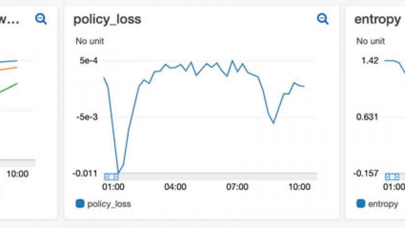
Amazon SageMaker RL saves the metadata associated with each training job, such as the instance used, the source code, and the metrics logged. The print logs are saved in Amazon CloudWatch, the training outputs are saved in Amazon Simple Storage Service (Amazon S3), and you can replicate each training job with a single click. The Amazon SageMaker RL training job console visualizes the instance resource use and training metrics, such as episode reward and policy loss.
The following example visualization shows the mean episode rewards, policy entropy, and policy loss over the training time. As the agent learns to take better actions, its rewards improve. The entropy indicates the randomness of the actions taken by the agent. Initially, the agent takes random actions to explore the state space, and the entropy is high. As the agent improves, its randomness and entropy reduce. The policy loss indicates the value of the loss function used by the RL algorithm to update the policy neural network. We use the PPO algorithm, which should remain close to zero during training.

Ray also creates a TensorBoard with training metrics and saves them to Amazon S3. The following visualizations show the same metrics in TensorBoard.


Ray is designed for distributed runs, so it can efficiently use all the resources available in an instance: CPU, GPU, and memory. You can scale the training further with multi-instance clusters by incrementing the train_instance_count in the preceding API call. Amazon SageMaker RL creates the cluster for you, and Ray uses cluster resources to train the agent rapidly.
You can choose to create heterogeneous clusters with multiple instance types (for more information, see the following GitHub repo). For more information about distributed RL training, see Scaling your AI-powered Battlesnake with distributed reinforcement learning in Amazon SageMaker.
You can scale your experiments by creating training jobs with different configurations of state representation, reward function, RL algorithms, hyperparameters, and more. Amazon SageMaker RL helps you organize, track, compare, and evaluate your training jobs with Amazon SageMaker Experiments. You can search, sort by performance metrics, and track the lineage of a policy when you deploy in production. The following code shows an example of experiments with multiple learning rates for training a policy, and sorting by the mean episode rewards:
# define a SageMaker Experiment
rl_exp = Experiment.create(experiment_name="learning_rate_exp",...)

# define first trial
first_trial = Trial.create(trial_name="lr-1e-3",
                           experiment_name=rl_exp.experiment_name,...)
estimator_1 = RLEstimator(...)
estimator_1.fit(experiment_config={"TrialName": first_trial.trial_name,...})

# define second trial
second_trial = Trial.create(trial_name="lr-1e-4",
                            experiment_name=rl_exp.experiment_name,...)
estimator_2 = RLEstimator(...)
estimator.fit(experiment_config={"TrialName": second_trial.trial_name,...})

# define third trial
third_trial = Trial.create(trial_name="lr-1e-5",
                            experiment_name=rl_exp.experiment_name,...)
estimator_3 = RLEstimator(...)
estimator.fit(experiment_config={"TrialName": third_trial.trial_name,...})

# get trials sorted by mean episode rewards
trial_component_analytics = ExperimentAnalytics(
    experiment_name=rl_exp.experiment_name,
    sort_by="metrics.episode_reward_mean.Avg",
    sort_order="Descending",...).dataframe()
The following screenshot shows the output.

The following screenshot shows that we saved 60% of the training cost by using a Spot Instance.

Deploying and monitoring the policy
After you train the RL policy, you can export the learned policy for evaluation and deployment. You can evaluate the learned policy against realistic scenarios expected in production, and ensure its behavior matches the expectation from domain expertise. You can deploy the policy in an Amazon SageMaker endpoint, to edge devices using AWS IoT Greengrass (see Training the Amazon SageMaker object detection model and running it on AWS IoT Greengrass – Part 3 of 3: Deploying to the edge), or natively in your production system.
Amazon SageMaker endpoints are fully managed. You deploy the policy with a single API call, and the required instances and load balancer are created behind a secure HTTP endpoint. The Amazon SageMaker endpoint autoscales the resources so that latency and throughput requirements are met with changing traffic patterns while incurring minimal cost.
With an Amazon SageMaker endpoint, you can check the policy performance in the production environment by A/B testing the policy against the existing model in production. You can log the decisions taken by the policy in Amazon S3 and check for anomalous behavior using Amazon SageMaker Model Monitor. You can use the resulting dataset to train an improved policy. If you have multiple policies, each for a different brand of basketball sold in the store, you can save on costs by deploying all the models behind a multi-model endpoint.
The following code shows how to extract the policy from the RLEstimator and deploy it to an Amazon SageMaker endpoint. The endpoint is configured to save all the model inferences using the Model Monitor feature.
endpoint_name = 'basketball-demo-model-monitor-' + strftime("%Y-%m-%d-%H-%M-%S", gmtime())
prefix = 'sagemaker/basketball-demo-model-monitor'
data_capture_prefix = '{}/datacapture'.format(prefix)
s3_capture_upload_path = 's3://{}/{}'.format(s3_bucket, data_capture_prefix)

model = Model(model_data='s3://{}/{}/output/model.tar.gz'.format(s3_bucket, job_name),
              framework_version='2.1.0',
              role=role)

data_capture_config = DataCaptureConfig(
                            enable_capture=True,
                            sampling_percentage=100,
                            destination_s3_uri=s3_capture_upload_path)

predictor = model.deploy(initial_instance_count=1,
                         instance_type="ml.c5.xlarge",
                         endpoint_name=endpoint_name,
                         data_capture_config=data_capture_config)

result = predictor.predict({"inputs": ...})
You can verify the configurations on the console. The following screenshot shows the data capture settings.

The following screenshot shows model’s production variants.

When the endpoint is up, you can quickly trace back to the model trained under the hood. The following code demonstrates how to retrieve the job-specific information (such as TrainingJobName, TrainingJobStatus, and TrainingTimeInSeconds) with a single line of API call:
#first get the endpoint config for the relevant endpoint
endpoint_config = sm.describe_endpoint_config(EndpointConfigName=endpoint_name)

#now get the model name for the model deployed at the endpoint.
model_name = endpoint_config['ProductionVariants'][0]['ModelName']

#now look up the S3 URI of the model artifacts
model = sm.describe_model(ModelName=model_name)
modelURI = model['PrimaryContainer']['ModelDataUrl']

#search for the training job that created the model artifacts at above S3 URI location
search_params={
   "MaxResults": 1,
   "Resource": "TrainingJob",
   "SearchExpression": {
      "Filters": [
         {
            "Name": "ModelArtifacts.S3ModelArtifacts",
            "Operator": "Equals",
            "Value": modelURI
         }]}
}
results = sm.search(**search_params)

# trace lineage of the underlying training job
results['Results'][0]['TrainingJob'].keys()
The following screenshot shows the output.

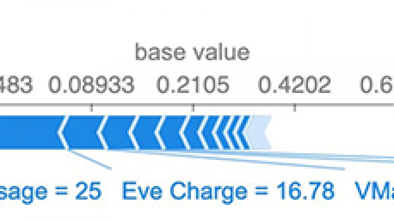
When you invoke the endpoint, the request payload, response payload, and additional metadata is saved in the Amazon S3 location that you specified in DataCaptureConfig. You should expect to see different files from different time periods, organized based on the hour when the invocation occurred. The format of the Amazon S3 path is s3://{destination-bucket-prefix}/{endpoint-name}/{variant-name}/yyyy/mm/dd/hh/filename.jsonl.
The HTTP request and response payload is saved in Amazon S3, where the JSON file is sorted by date. The following screenshot shows the view on the Amazon S3 console.

The following code is a line from the JSON file. With all the captured data, you can closely monitor the endpoint status and perform evaluation when necessary.
'captureData': {
    'endpointInput': {
        'data':
            {"inputs": {
                "observations":
                    [[1307.4744873046875, 737.0364990234375,
                    2065.304931640625, 988.8933715820312,
                    357.6395568847656, 41.90699768066406,
                    60.84299850463867, 4.65033483505249,
                    5.944803237915039, 64.77123260498047]],
                "prev_action": [0],
                "is_training": false,
                "prev_reward": -1,
                "seq_lens": -1}},
        'encoding': 'JSON',
        'mode': 'INPUT',
        'observedContentType': 'application/json'},
    'endpointOutput': {
        'data': {
            "outputs": {
                "action_logp": [0.862621188],
                "action_prob": [2.36936307],
                "actions_0": [[-0.267252982]],
                "vf_preds": [0.00718466379],
                "action_dist_inputs": [[-0.364359707, -2.08935]]
            }
        },
        'encoding': 'JSON',
        'mode': 'OUTPUT',
        'observedContentType': 'application/json'}}
'eventMetadata': {
        'eventId': '0ad69e2f-c1b1-47e4-8334-47750c3cd504',
        'inferenceTime': '2020-09-30T00:47:14Z'
        },
'eventVersion': '0'
Conclusion
With Ray and Amazon SageMaker RL, you can get started on reinforcement learning quickly and scale to production workloads. The total cost of ownership of Amazon SageMaker over a 3-year horizon is reduced by over 54% compared to other cloud options, and developers can be up to 10 times more productive.
The post just scratches the surface of what you can do with Amazon SageMaker RL. Give it a try and please send us feedback, either in the Amazon SageMaker Discussion Forum or through your usual AWS contacts.
About the Author
 Bharathan Balaji is a Research Scientist in AWS and his research interests lie in reinforcement learning systems and applications. He contributed to the launch of Amazon SageMaker RL and AWS DeepRacer. He likes to play badminton, cricket and board games during his spare time.
 Anna Luo is an Applied Scientist in AWS. She obtained her Ph.D. in Statistics from UC Santa Barbara. Her interests lie in large-scale reinforcement learning algorithms and distributed computing. Her current personal goal is to master snowboarding.


 Yotam Elor is a Senior Applied Scientist at AWS Sagemaker. He works on
  Somnath Sarkar is a Software Engineer in the AWS SageMaker Autopilot team. He enjoys machine learning in general with focus in scalable and distributed systems.


 So Young Yoon is a Conversation A.I. Architect at AWS Professional Services where she works with customers across multiple industries to develop specialized conversational assistants which have helped these customers provide their users faster and accurate information through natural language. Soyoung has M.S. and B.S. in Electrical and Computer Engineering from Carnegie Mellon University.


 Priyanka Gopalakrishna is a software engineer at Amazon AI. Her focus is on solving labeling problems using machine learning and building scalable AI solutions using distributed systems.
 Talia Chopra is a Technical Writer in AWS specializing in machine learning and artificial intelligence. She works with multiple teams in AWS to create technical documentation and tutorials for customers using Amazon SageMaker, MxNet, and AutoGluon.